Article

Subpixel-Scale Topography Retrieval of Mars Using Single-Image DTM Estimation and Super-Resolution Restoration

1
Imaging Group, Mullard Space Science Laboratory, Department of Space and Climate Physics, University College London, Holmbury St Mary, Surrey RH5 6NT, UK
2
College of Civil and Transportation Engineering, Shenzhen University, Shenzhen 518060, China
3
Ministry of Natural Resources Key Laboratory for Geo-Environmental Monitoring of Great Bay Area & Guangdong Key Laboratory of Urban Informatics & Shenzhen Key Laboratory of Spatial Smart Sensing and Services, Shenzhen University, Shenzhen 518060, China
4
Department of Geosciences, Institute for Geological Sciences, Planetary Sciences and Remote Sensing, Freie Universität Berlin, 12249 Berlin, Germany
5
Laboratoire de Planétologie et Géodynamique, CNRS, UMR 6112, Université de Nantes, 44300 Nantes, France
6
Joanneum Research, Steyrergasse 17, 8010 Graz, Austria
7
INAF, Osservatorio Astronomico di Padova, 35122 Padova, Italy
8
Physikalisches Institut, Universität Bern, Siedlerstrasse 5, 3012 Bern, Switzerland
*
Author to whom correspondence should be addressed.
Submission received: 13 December 2021 / Revised: 22 December 2021 / Accepted: 29 December 2021 / Published: 6 January 2022
(This article belongs to the Special Issue Planetary 3D Mapping, Remote Sensing and Machine Learning)

Abstract

:
We propose using coupled deep learning based super-resolution restoration (SRR) and single-image digital terrain model (DTM) estimation (SDE) methods to produce subpixel-scale topography from single-view ESA Trace Gas Orbiter Colour and Stereo Surface Imaging System (CaSSIS) and NASA Mars Reconnaissance Orbiter High Resolution Imaging Science Experiment (HiRISE) images. We present qualitative and quantitative assessments of the resultant 2 m/pixel CaSSIS SRR DTM mosaic over the ESA and Roscosmos Rosalind Franklin ExoMars rover’s (RFEXM22) planned landing site at Oxia Planum. Quantitative evaluation shows SRR improves the effective resolution of the resultant CaSSIS DTM by a factor of 4 or more, while achieving a fairly good height accuracy measured by root mean squared error (1.876 m) and structural similarity (0.607), compared to the ultra-high-resolution HiRISE SRR DTMs at 12.5 cm/pixel. We make available, along with this paper, the resultant CaSSIS SRR image and SRR DTM mosaics, as well as HiRISE full-strip SRR images and SRR DTMs, to support landing site characterisation and future rover engineering for the RFEXM22.

1. Introduction

Mars is the most Earth-like planet within our solar system and is probably the Earth’s closest habitable neighbour. In order to develop an in-depth understanding of our neighbouring planet for future human exploration, we need to better understand the different Martian surface geologies, processes, features and phenomena. Critical to this endeavour has been the role of remotely sensed images since the first successful flyby mission in 1965 by Mariner IV [1], and over the last 56 years via multiple orbital (e.g., [2,3,4,5,6]) and robotic (e.g., [7,8,9,10]) missions. Amongst all the data collected and derived through these missions, high-resolution digital terrain models (DTMs) and their corresponding terrain-corrected orthorectified images (ORIs) are probably two of the most important resources for studying the Martian surface as well as its interaction with the Martian atmosphere.
Apart from the globally available lower resolution (~463 m/pixel) Mars Orbiter Laser Altimeter (MOLA) DTM [11,12], higher resolution Mars DTMs are typically produced from the 12.5–50 m/pixel Mars Express High Resolution Stereo Camera (HRSC) images [13], the 6 m/pixel Mars Reconnaissance Orbiter (MRO) Context Camera (CTX) images [14], the ~4.6 m/pixel (4 m/pixel nominal resolution) ExoMars Trace Gas Orbiter (TGO) Colour and Stereo Surface Imaging System (CaSSIS) images [15,16], and the ~30 cm/pixel (25 cm/pixel nominal resolution) MRO High Resolution Imaging Science Experiment (HiRISE) images [17]. The DTM products derived from these imaging sources often have different effective resolutions and spatial coverage, depending on the properties of the input images and the DTM retrieval methods, which include traditional photogrammetric methods [18,19,20,21], photoclinometry methods [22,23,24,25], and deep learning-based methods [26,27,28,29].
It has been a common understanding that DTMs derived from a particular imaging dataset can only achieve a lower, or at the best, similar effective spatial resolution compared to the input images, due to the various approximations and/or filtering processes introduced by the photogrammetric or photoclinometric pipelines. With recent successes in deep learning techniques, it has now become more practical and effective to improve the effective resolution of an image using super-resolution restoration (SRR) networks [30], retrieving pixel-scale topography using single-image DTM estimation (SDE) networks [27,29], and eventually, combining the two techniques to potentially produce subpixel-scale topography from only a single-view input image.
SRR refers to the process of improving the spatial resolution and retrieving high-frequency details from a given lower-resolution image by combining subpixel or multi-angle [31,32,33] information contained in multiple lower-resolution inputs, or through inference of the best possible higher-resolution solution using deep learning techniques [30,34,35,36]. In particular, the deep learning-based SRR methods, either using residual networks [37,38,39], recursive networks [40,41], attention-based networks [42,43], and/or using generative adversarial networks (GANs) [44,45,46], have become more and more popular over the last decade, not only in the field of picture/photo enhancement, but also in the field of Earth observation for improving the quality and resolution of satellite imagery [34,35,36].
In parallel, SDE refers to the process of deriving heights or depths from a given single-view image, using traditional “shape from shading” (photoclinometry) techniques [22,23,24,47,48], or learning the “height/depth cues” from a training dataset using deep learning techniques. Such deep learning-based SDE methods, using residual networks [49,50,51], conditional random fields [52,53,54,55], attention-based networks [56,57], GANs [58,59], and U-nets [60,61], have been fairly successful in recent years, not only in the field of indoor/outdoor scene reconstruction but also in the field of remote sensing for topographic retrieval using planetary orbital images [26,27,28,29].
In this paper, we propose combining the use of SRR and SDE to boost the effective resolution of optical single-image-based DTMs to subpixel-scale. The in-house implementations of the MARSGAN (multi-scale adaptive-weighted residual super-resolution generative adversarial network) SRR system [30,35] and the MADNet (multi-scale generative adversarial U-net based single-image DTM estimation) SDE system [27,29] are employed for this study. Our study site is within the 3-sigma ellipses of the Rosalind Franklin ExoMars rover’s planned landing site (centred near 18.275°N, 335.368°E) at Oxia Planum [28,62,63]. We use the 4 m/pixel TGO CaSSIS “PAN” band images [15] and the 25 cm/pixel MRO HiRISE “RED” band images [17] as the input test datasets. We apply MARSGAN SRR to the original CaSSIS and HiRISE images, and subsequently, we apply MADNet SDE to the resultant 1 m/pixel CaSSIS SRR images and the 6.25 cm/pixel HiRISE SRR images, to produce CaSSIS SRR-DTMs at 2 m/pixel and HiRISE SRR-DTMs at 12.5 cm/pixel, respectively.
We show qualitative assessments for the resultant CaSSIS and HiRISE SRR-DTMs. We also provide quantitative assessments for the CaSSIS SRR-DTMs using the DTM evaluation technique that is described in [64], using multiple smoothed versions of the higher-resolution reference DTMs to compare with the lower-resolution target DTMs. The 1 m/pixel HiRISE Planetary Data System (PDS) DTMs (available through the University of Arizona HiRISE archive at https://www.uahirise.org/dtm/(accessed on 22 December 2021)) and the 50 cm/pixel HiRISE MADNet DTMs [28] (available through the ESA Guest Storage Facility (GSF) at https://www.cosmos.esa.int/web/psa/ucl-mssl_oxia-planum_hrsc_ctx_hirise_madnet_1.0 (accessed on 22 December 2021)) are tested, but their effective resolutions are inadequate (not high enough) to evaluate the CaSSIS SRR-DTMs as detailed in Section 3. We use instead the 12.5 cm/pixel HiRISE SRR-DTMs to compare with the CaSSIS SRR-DTMs, as well as performing “inverse” comparisons for the HiRISE PDS DTMs and HiRISE MADNet DTMs with respect to the HiRISE SRR-DTMs to yield quantitative analysis. Root mean squared error (RMSE) and the structural similarity index measurement (SSIM) [65] are used here as the evaluation metrics.
We publish the final products as area mosaics of 2 m/pixel CaSSIS SRR-DTMs and 1 m/pixel CaSSIS greyscale and colour ORIs of the ExoMars Rosalind Franklin rover’s landing site at Oxia Planum [62,63]. The NASA Ames Stereo Pipeline software [19] is used to blend and produce a mosaic of the resultant single-strip CaSSIS SRR-DTMs. In-house photometric correction and mosaicing software [21,66] is used to produce an image mosaic from the resultant single-strip CaSSIS SRR images. In addition, we also show examples of full-strip 6.25 cm/pixel HiRISE SRR ORIs and 12.5 cm/pixel HiRISE SRR MADNet DTMs produced from the 25 cm/pixel HiRISE “RED” band PDS ORIs. The resultant CaSSIS SRR and SRR-DTM products have been delivered to the ExoMars PanCam team for multi-resolution and ultra-high-resolution 3D visualisation using PRo3D [67,68]. The resultant CaSSIS, HiRISE SRR and DTM products are submitted as supporting material and are being published through the ESA GSF archive [69,70] (see https://www.cosmos.esa.int/web/psa/ucl-mssl_meta-gsf (accessed on 22 December 2021)).
The layout of the rest of the paper is as follows. In Section 2.1, we introduce the main datasets from CaSSIS and HiRISE. In Section 2.2, we revisit the MARSGAN SRR and MADNet SDE methods, and introduce the training details, followed by an explanation of the processing and DTM evaluation methods in Section 2.3. In Section 3.1, we give an overview of the CaSSIS SRR and SDE results, followed by qualitative assessments of the CaSSIS SRR and SDE results in Section 3.2, and qualitative assessments of the HiRISE SRR and SDE results in Section 3.3. In Section 3.4, we show quantitative evaluation of the CaSSIS and HiRISE DTM products. In Section 4, we discuss issues and uncertainties before drawing conclusions in Section 5.

2. Materials and Methods

2.1. Datasets

TGO CaSSIS is a moderately high-resolution, multispectral (from ~500 nm to ~950 nm for visible and near-infrared (NIR)), push-frame (an intermediate between a line scan camera and a framing camera) stereo imager, with the goal of extending the coverage of the MRO HiRISE camera and to produce moderately high-resolution DTMs of the Martian surface [15]. CaSSIS provides colour images consisting of the “BLU” band (centred at 499.9 nm for blue-green), the “PAN” band (centred at 675.0 nm for orange-red), the “RED” band (centred at 836.2 nm for NIR), and the “NIR” band (centred at 936.7 nm for NIR) [16]. Due to the limitation on the data transfer time, CaSSIS generally collects colour images from three out of the four bands at lower spacecraft altitudes (where ground velocity is higher), and all four bands only at higher altitudes (both with width reduction for some of the colour bands). CaSSIS images are typically sampled at 4 m/pixel nominal spatial resolution (~4.6 m/pixel effective spatial resolution) with a swath width of about 9.5 km and a swath length of about 30–40 km. Due to the non-sun-synchronous orbit and its 74° inclination angle, CaSSIS is able to image sites at different local times of different seasons, making CaSSIS images an ideal dataset for studying the Martian surface changes. At the time of the writing of this paper, CaSSIS images covered 4.3% of the Martian surface (by 28 August 2021).
In contrast, MRO HiRISE is designed to image very fine-scale surface features of Mars at 25 cm/pixel nominal spatial resolution (~30 cm/pixel effective spatial resolution), with a smaller swath width of about 6 km (for panchromatic) and 1.2 km (for colour), but a larger swath length of up to 60 km [17]. HiRISE collects images in three colour bands, consisting of a red band (centred at 694 nm), a blue-green band (centred at 536 nm), and an NIR band (centred at 874 nm), with the blue-green and NIR bands having much narrower swath widths compared to the red band images. Currently, HiRISE images (from 2007 to 2 September 2021) cover a smaller area (~3.4%) of the Martian surface in comparison to the coverage of CaSSIS (~4.3%). Figure 1 shows the footprints of the HiRISE (blue, foreground) and CaSSIS (green, background) images (in Mollweide projection–see https://pro.arcgis.com/en/pro-app/latest/help/mapping/properties/mollweide.htm (accessed on 22 December 2021)), up to 2 September 2021 and 28 August 2021, respectively.
In this work, we experiment with the TGO CaSSIS PAN band images over the ESA and Roscosmos Rosalind Franklin ExoMars rover’s landing site at Oxia Planum [28,62,63]. Up until 28 August 2021, CaSSIS has 100% coverage for the 1-sigma landing ellipses, about 92% coverage for the 3-sigma landing ellipses, and about 67% for the ExoMars team’s geological characterisation area [71] of the landing site. Table 1 lists the test CaSSIS images (selected for non-repeat coverage), available overlapping HiRISE PDS DTMs and ORIs that are used later on for comparison/evaluation and to produce the HiRISE SRR MADNet DTMs. A previously produced 50 cm/pixel HiRISE MADNet DTM mosaic consisting of 44 HiRISE single-strip DTMs (available through ESA GSF; link is provided in Section 1) [28], which has a 100% coverage of the 3-sigma landing ellipses, is also used for intercomparisons. It should be noted that both of the HiRISE PDS DTMs and the HiRISE MADNet DTM mosaic were previously 3D co-aligned with respect to the cascaded 12 m/pixel CTX and 25 m/pixel HRSC MADNet DTM mosaics [28] that are both available through the same ESA link, which themselves are co-aligned with the United States Geological Survey (USGS) MOLA areoid DTM v.2 (available at https://astrogeology.usgs.gov/search/details/Mars/GlobalSurveyor/MOLA/Mars_MGS_MOLA_DEM_mosaic_global_463m/cub (accessed on 22 December 2021)). Figure 2 shows an overview map of the test CaSSIS images (co-registered with the CTX and HRSC ORIs [28]) superimposed on the baseline referencing CTX MADNet DTM mosaic [28].

2.2. Overview of MARSGAN SRR and MADNet SDE

MARSGAN [30] and MADNet [29] are both based on the relativistic GAN framework [72,73] that involves training of a generator network and a relativistic discriminator network in parallel. For MARSGAN SRR, the generator network is trained to produce potential SRR estimations, whilst the discriminator network is trained in parallel (and updated in an alternating manner with the generator network) to estimate the probability of the given training higher-resolution images being relatively more realistic than the generated SRR images on average (within a small batch), whereas for MADNet SDE, the generator network is trained to produce per-pixel relative heights, and the discriminator network is trained to distinguish the predicted heights from the ground-truth heights.
For the MARSGAN generator network, a feed-forward residual convolutional neural network architecture is employed, consisting of twenty-three adaptive weighted residual-in-residual dense blocks, followed by an adaptive weighted multi-scale reconstruction block [30]. Each of the adaptive weighted residual-in-residual dense blocks contains eleven independent weights, three dense convolution blocks [74], and additive noise inputs on top of the residual-in-residual structure. For the MADNet generator network, a fully convolutional U-net [75] architecture is employed, consisting of four stacks of dense convolution blocks as the encoder and five stacks of up-projection blocks [51] as the decoder. MARSGAN and MADNet use a similar discriminator network architecture as detailed in [29,30,44]. Simplified network architectures of the MARSGAN SRR and MADNet SDE networks that are used in this work are shown in Figure 3.
For training, MARSGAN uses a weighted sum of the mean absolute error and mean squared error (MSE) based content loss, lower-level and higher-level VGG (named after the Visual Geometry Group at the University of Oxford) feature [76] based perceptual loss, and the relativistic adversarial [73] loss. The total loss function of MARSGAN ensures the network is trained towards a “balanced” SRR solution combining perceptual-driven enhancement and pixelwise difference-based enhancement. In [30], the MARSGAN model was trained with a collection of down-sampled (1 m/pixel) HiRISE PDS ORIs (lower-resolution training samples) and full-resolution (25 cm/pixel) HiRISE PDS ORIs (higher-resolution training samples). In this work, we retrain the MARSGAN model based on the initial study of the “real-world” image degradation that is described in [77], and our previous study of SRR of Earth observation imagery [35], wherein we demonstrated the positive impact of using a post-processed training dataset to improve the SRR quality and to minimise synthetic artefacts.
The “post-processing” of the training dataset that is employed in this work contains three aspects. Firstly, the original HiRISE training samples (lower-resolution and higher-resolution; from [30]) are manually screened and lower-quality samples are removed from the training dataset. Secondly, we down-sample the higher-resolution HiRISE training samples from 25 cm/pixel into 50 cm/pixel to reduce the native noise (e.g., stripes or fixed pattern noise) that is commonly found when zooming in to 100% display of the 25 cm/pixel HiRISE samples, and subsequently, the lower-resolution HiRISE training samples are down-sampled from 1 m/pixel into 2 m/pixel to form the lower-resolution counterpart of the training dataset. Thirdly, a sequence of weighted median, bilateral filtering, and Gaussian blurring is applied to the lower-resolution HiRISE training samples to simulate the blurring effect of lower-resolution images, instead of using only the bicubic down-sampling process on the higher-resolution counterpart, as this was demonstrated as being insufficient and inappropriate to model the degradations of orbital and real-world images [35,77].
On the other hand, MADNet uses a weighted sum of the Berhu loss [78], the image gradient loss, and the relativistic averaged adversarial loss. The total loss function of MADNet ensures the network learns optimal DTM estimation combining pixelwise-difference guided prediction and structural similarity penalised retrieval. The MADNet model [29] was trained with a selected collection of down-sampled (at 2 m/pixel and 4 m/pixel) HiRISE PDS ORIs and DTMs and down-sampled (36 m/pixel) CTX iMars ORIs and DTMs [20,29]. In this work, we use the pretrained MADNet model [29] for relative DTM inference but we do not use the multi-scale reconstruction procedure that is employed in [29]. This is because the resolution difference between the target CaSSIS image (4 m/pixel) and the reference CTX MADNet DTM (12 m/pixel), as well as the resolution difference between the target CaSSIS SRR image (1 m/pixel) and the reference CaSSIS MADNet DTM (4 m/pixel) that are used in this work, are much smaller than the resolution difference between the target HiRISE image (25 cm/pixel) and the reference CTX MADNet DTM (12 m/pixel) that are used in the previous work [28,29]. We set the final CaSSIS MADNet DTM products at 8 m/pixel and the CaSSIS SRR MADNet DTM products at 2 m/pixel, i.e., half the resolution of the input image, to minimise the resolution gap between the output and the reference DTMs, whilst on the other hand, without the multi-scale reconstruction process, we obtain a better completeness of the CaSSIS SRR MADNet DTM coverage (about 88% rather than 76% due to using a fixed tile size on much smaller-sized down-sampled images) of the 3-sigma ellipses of the ExoMars landing site, and also, within a short processing time (less than 22 h in total).

2.3. DTM Evaluation

We perform qualitative and quantitative assessments for the resultant CaSSIS SRR-DTMs, but only qualitative evaluation for the resultant HiRISE SRR-DTMs. For qualitative evaluation, we perform visual inspection of the resultant target DTMs in comparison with other reference DTMs from different data sources at different resolutions that are co-aligned with the same baseline DTM, i.e., the USGS MOLA areoid DTM. Comparison of shaded relief images computed from the target and reference DTMs and their corresponding ORIs is performed to obtain qualitative insights on the level of details and overall quality of the target DTMs, to assess the smallest areal features that can be observed from both the target DTMs and the reference ORIs, and to inspect if there are any systematic or local errors/artefacts from the target DTMs.
On the other hand, quantitative evaluation of high-resolution Mars topographic products (≤10 m/pixel) is always a difficult task as there are currently no high-resolution, high-accuracy and large spatial coverage topographic data that can be considered as “ground-truth” available for Mars. A recent Mars DTM evaluation study [64] examined the relative effective resolution and accuracy of target DTMs (at lower nominal resolutions, i.e., 20–50 m/pixel from CTX and HRSC) with respect to a set of reference DTMs (at higher nominal resolution, i.e., ~1 m/pixel from HiRISE) that are considered as having much higher effective resolution and vertical accuracy (20 times or more) than the target DTMs. This assumption is made based on the conjecture that even though the differences between the target and reference DTMs arise from errors of both datasets, the errors of the reference dataset can be considered as negligible due to the reference DTMs having much higher resolution (as much smaller features can be resolved) and thus much higher accuracy than the target DTM. The authors in [64] suggest that even a smaller ratio would likely suffice, the “ideal” reference DTMs should have 20 times or higher resolution and vertical precision than the target DTMs.
As described in [64], a sequence of boxcar low-pass filters with increasing kernel sizes (3 × 3, 5 × 5, 7 × 7, …) are used to smooth the reference DTM. Subsequently, the smoothed versions of the reference DTM are compared with the target DTM one by one, and from which, we can expect that the RMSE differences will first decrease as features that the target DTM fails to resolve are removed, then increase as larger filters begin to remove features that are present in the target DTM. Eventually, the relative effective resolution can be defined quantitatively in terms of the smoothing kernel size that yields the minimum RMSE, and this minimum RMSE is hypothesized to characterise the accuracy of the target DTM.
In this work, we follow the same method to quantitatively evaluate the resultant 8 m/pixel CaSSIS DTMs and 2 m/pixel CaSSIS SRR-DTMs (target DTMs) using multiple smoothed versions of the 12.5 cm/pixel HiRISE SRR-DTMs (reference DTMs). We add the SSIM [65] scoring that measures the differences between structural features as an additional evaluation metric to complement and support the pixelwise difference measurements from RMSE. The overall evaluation workflow (as shown in Figure 4) consists of four steps (similar to [64]), including (a) map reprojection, down-sampling, and 3D co-alignment of the reference DTMs to match with the target DTMs; (b) applying odd-sized boxcar filters (i.e., 3 × 3, 5 × 5, 7 × 7, …) to smooth out the details of the reference DTMs; (c) masking out no-data and non-overlapping areas; and (d) calculating RMSEs and SSIMs for all valid overlapping DTM areas.

3. Results

3.1. Overview of the CaSSIS SRR and SDE Results and Product Access Information

In this work, we have produced nine single-strip CaSSIS PAN band (see Table 1 for image IDs) 1 m/pixel SRR images and 2 m/pixel SRR-DTMs, a brightness and contrast corrected 1 m/pixel CaSSIS SRR greyscale image mosaic, a 1 m/pixel CaSSIS SRR colour image mosaic (colourised using HRSC colour due to the CaSSIS colour bands being much narrower than the PAN band), an 8 m/pixel CaSSIS DTM mosaic, and a 2 m/pixel CaSSIS SRR-DTM mosaic, over the 3-sigma ellipses of the ExoMars Rosalind Franklin rover’s planned landing site at Oxia Planum. Figure 5 shows overview maps of the original 4 m/pixel CaSSIS NPB (NIR-PAN-BLU) band colour images, the resultant 1 m/pixel CaSSIS PAN band SRR single-strip images, 1 m/pixel CaSSIS SRR image mosaic, 1 m/pixel CaSSIS SRR image mosaic with HRSC colour (through intensity-hue-saturation (I-H-S) pan-sharpening), 8 m/pixel CaSSIS MADNet DTM mosaic and the shaded relief image (330° azimuth, 30° altitude, 2× vertical exaggeration), and the 2 m/pixel CaSSIS SRR MADNet DTM mosaic and the shaded relief image (330° azimuth, 30° altitude, 2× vertical exaggeration). It should be noted that all CaSSIS SRR, MADNet DTM, and SRR MADNet DTM results are produced using the 4 m/pixel CaSSIS PAN band images, the 4 m/pixel CaSSIS NPB colour images that are shown in Figure 5 are for information only to show their narrower coverage and the reason why they are not used in this work (gaps between the adjacent colour images). It should also be noted that the gaps in the 8 m/pixel CaSSIS MADNet DTM mosaic are due to using a fixed tile size (512 × 512 pixels) without any no-data value at the edges of the two barely overlapped CaSSIS PAN band images. The gaps are eliminated in the 2 m/pixel CaSSIS SRR MADNet DTM mosaic using the much larger 1 m/pixel CaSSIS SRR images.
The above results (SRR image and SRR-DTM) are at a very high resolution with uniform quality and consistency and are being published through the ESA GSF. They are spatially co-registered and vertically co-aligned with respect to the cascaded HiRISE, CTX, and HRSC ORIs and DTM mosaics that are described in [28], which themselves are accurately co-registered with the ESA/DLR/FUB HRSC MC-11W level 5 ORI mosaic (available at http://hrscteam.dlr.de/HMC30 (accessed on 22 December 2021)), and vertically co-aligned with the aforementioned USGS MOLA areoid DTM. We use identical map projection system (Equidistant Cylindrical/Equirectangular) and map projection parameters as used in the ESA/DLR/FUB HRSC MC-11W level 5 ORI and DTM products. We strongly recommend that readers download the resultant products from ESA GSF and look at fine-scale details (they are also provided as supporting material for review purpose), since only very small exemplar areas (i.e., “Zoom-in Area-1” and “Zoom-in Area-2” in Figure 6) of the results are shown here in Section 3.2 and Section 3.3.

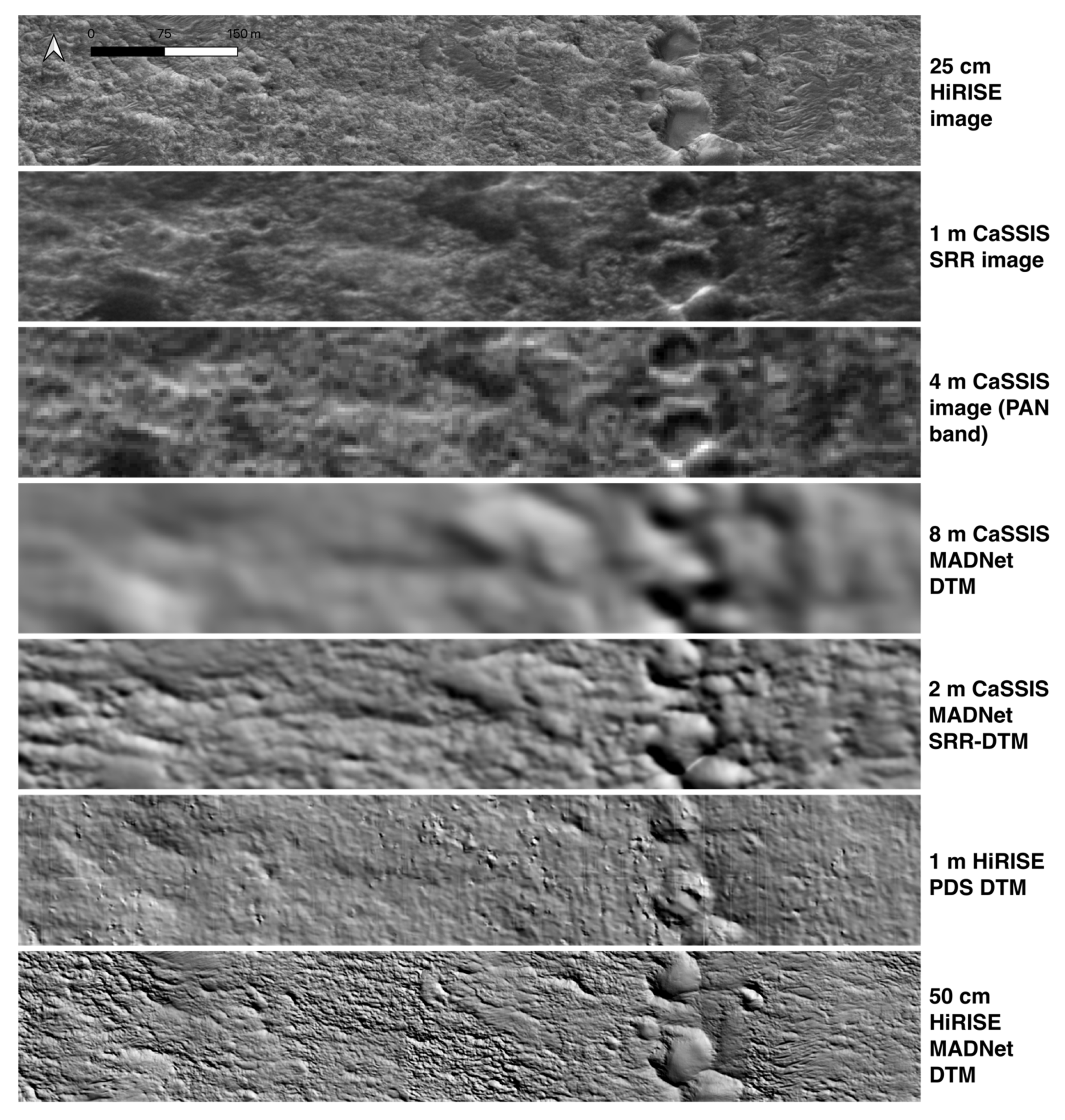
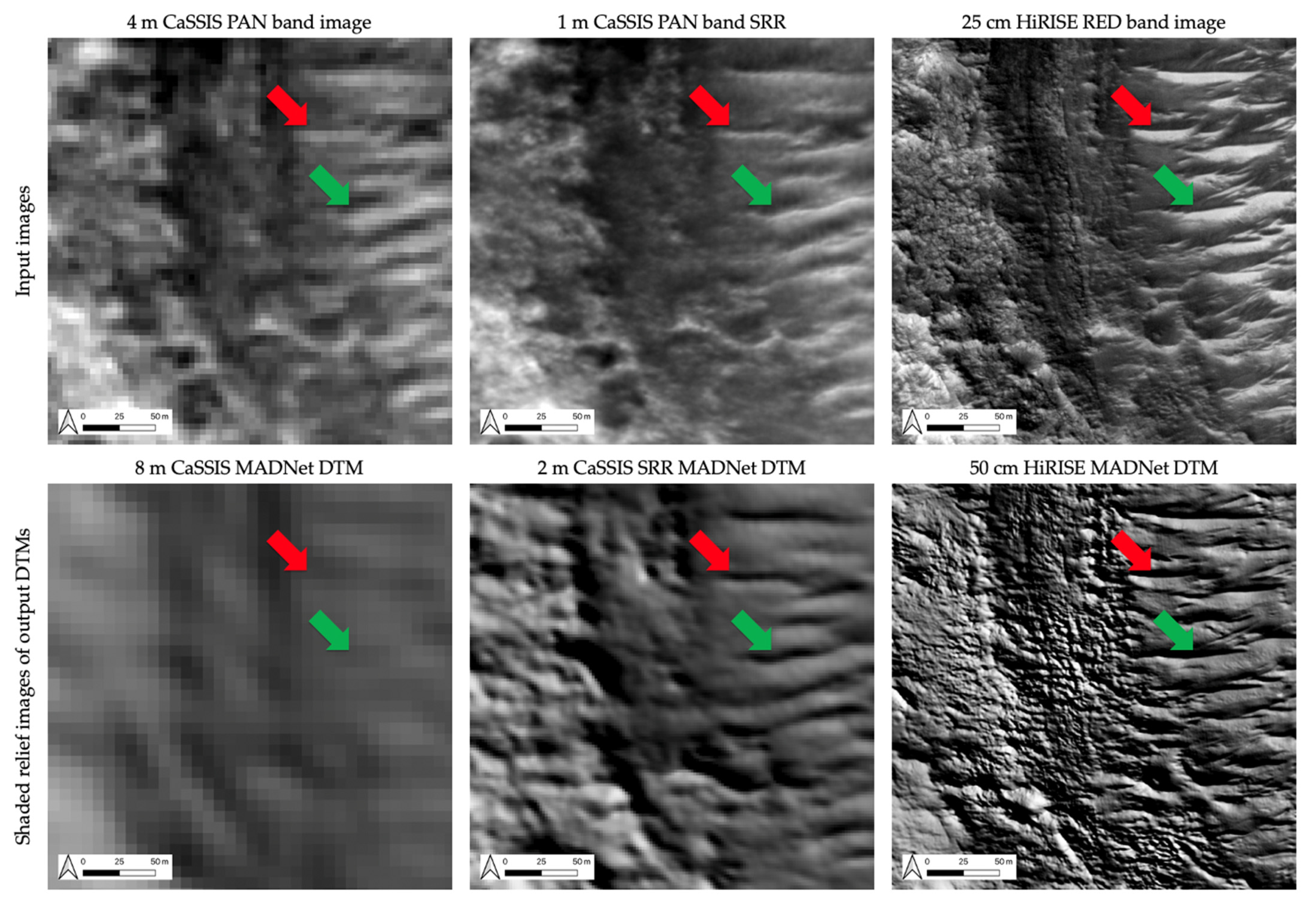
3.2. Qualitative Assessment of the CaSSIS SRR ORI and SRR MADNet DTM

In this work, we perform qualitative assessment (visual inspections) for both the resultant 1 m/pixel CaSSIS SRR images and 2 m/pixel CaSSIS SRR MADNet DTMs. The CaSSIS SRR results are visually inspected both at a large-scale and at different small-scales with multiple random zoom-in areas, and are compared with the original 4 m/pixel input CaSSIS PAN band images and the 25 cm/pixel HiRISE images, wherever they overlap. We have the following observations: (a) the CaSSIS SRR images have no systematic nor any patterned artefacts; (b) surface features on the CaSSIS SRR images are visually much clearer and sharper without changing the brightness or contrast of the original CaSSIS images; (c) there are no overshoot or undershoot issues at high-contrast edges; (d) image noise from the original CaSSIS images has been significantly reduced; (e) surface features/textures on the CaSSIS SRR images are much more comparable with respect to the surface features/textures on the HiRISE images, compared to the original CaSSIS images, although the HiRISE images still show much more details compared to the CaSSIS SRR images; and (f) some features have a different appearance between the CaSSIS SRR images and HiRISE images due to illumination and contrast differences, as they look similar to the same features shown in the CaSSIS SRR images when comparing to the original CaSSIS images.
The CaSSIS SRR MADNet DTM is also visually inspected at a large-scale and at different small-scales with multiple random zoom-in areas and is compared with the 8 m/pixel CaSSIS MADNet DTM mosaic, the 1 m/pixel HiRISE PDS DTMs, the 50 cm/pixel HiRISE MADNet DTM mosaic, as well as the CaSSIS and HiRISE images. Both colourised DTMs and shaded relief images are used in our visual inspection, and subsequently, we have the following observations: (a) there are significantly more improvements (higher levels of detail) between the CaSSIS MADNet DTM and the CaSSIS SRR MADNet DTM, compared to the improvement between the CaSSIS images and CaSSIS SRR images; (b) there are no observable systematic or local DTM artefacts/errors when/if comparing to the CaSSIS and SRR images; (c) there are quite a great deal of small topographic features that can now be observed in the CaSSIS SRR DTM and can also be identified (with similar appearance) from the HiRISE DTMs, however, there are also small topographic features that are shown on the CaSSIS SRR MADNet DTM, which have slightly different appearance in the HiRISE DTMs; (d) some small topographic features that are resolved in the CaSSIS SRR MADNet DTM appear to be realistic when comparing to the CaSSIS and CaSSIS SRR images, but less realistic when compared to the HiRISE images; (e) ignoring the apparent artefacts from the HiRISE PDS DTMs, the CaSSIS SRR MADNet DTM appears to have similar features present but at a much higher effective resolution and details comparable to the HiRISE PDS DTMs, but with lower effective resolution and details comparable to the HiRISE MADNet DTM; and (f) the high-frequency noise from the original CaSSIS images does not results in any DTM artefact, but it does seem to have a negative impact on the effective resolution and resolvable details of the resultant CaSSIS MADNet DTM, which consequently highlights the better effective resolution and resolved topographic details from the CaSSIS SRR MADNet DTM benefiting from the CaSSIS SRR images being less noisy.
Figure 7 shows a small exemplar area (refer to “Zoom-in Area-1” in Figure 6 for its location) of the CaSSIS SRR MADNet DTM mosaic that overlaps with the HiRISE PDS DTM (DTEEC_039299_1985_047501_1985_L01), demonstrating the different level of details of the 25 cm/pixel HiRISE PDS ORI (ESP_039299_1985_RED_A_01_ORTHO), the 1 m/pixel CaSSIS SRR image, the 4 m/pixel original CaSSIS PAN band image (MY34_004925_019_2_PAN), the shaded relief images of the 8 m/pixel CaSSIS MADNet DTM, 2 m/pixel CaSSIS SRR MADNet DTM, 1 m/pixel HiRISE PDS DTM, and the 50 cm/pixel HiRISE MADNet DTM. We can observe that using the proposed MARSGAN SRR and MADNet SDE processing, the visual quality and details of the CaSSIS DTM has been significantly improved. The resultant 2 m/pixel CaSSIS SRR-DTM is much superior to the 8 m/pixel CaSSIS DTM and even has better visual quality and less noise in comparison with the 1 m/pixel HiRISE PDS DTM, while the “new” topographic features have a reasonable visual correlation in comparison with the 50 cm/pixel HiRISE MADNet DTM as well as the original HiRISE and CaSSIS images.

3.3. Qualitative Assessments of the HiRISE SRR and SRR MADNet DTMs

In addition to the CaSSIS results, we also processed five single-strip 25 cm/pixel HiRISE ORIs (see Table 1 for image IDs) into 6.25 cm/pixel HiRISE SRR images and 12.5 cm/pixel HiRISE SRR MADNet DTMs. Due to the large data volume, only two resultant full-strip HiRISE SRR MADNet DTM (ESP_039299_1985–the one shown in the examples and ESP_036925_1985) are currently available in the supporting material, more HiRISE SRR MADNet DTM results will be published through the ESA GSF. Overall, the improvement between the HiRISE and HiRISE SRR images, as well as improvement between the HiRISE MADNet DTM and the HiRISE SRR MADNet DTM are both visually obvious. The topographic features that are shown in the 12.5 cm/pixel HiRISE SRR MADNet DTM visually co-align with the image features that are shown in the 25 cm/pixel HiRISE and the 6.25 cm/pixel HiRISE SRR images.
Figure 8 shows a zoom-in view of a subarea (over the southern ridge of the larger crater on the northeast area; refer to “Zoom-in Area-2” in Figure 6 for its location) of the larger extent that is shown in Figure 7. We can observe that the peaks shown in the 12.5 cm/pixel HiRISE SRR MADNet DTM are visually much sharper than the same features that are shown in the 50 cm/pixel HiRISE MADNet DTM and 25 cm/pixel HiRISE image. On the other hand, small surface details are revealed in the 6.25 cm/pixel HiRISE SRR image, and their associated topography is revealed in the 12.5 cm/pixel HiRISE SRR MADNet DTM. The proposed technique is observed to have a better positive impact on improving the resolution and quality of the DTMs compared to improving the resolution and quality of the images themselves. We cannot quantitatively determine the resolution improvement and accuracy of the HiRISE SRR-DTM results as there are no higher spatial resolution ground-truth topographic data available at this site. However, assuming the same technique performs similarly to CaSSIS and to the HiRISE data, we can get some idea on the resolution and accuracy through quantitative assessments of the CaSSIS SRR-DTM results, which are described in the next section.

3.4. Quantitative Assessment of the CaSSIS SRR MADNet DTM

As discussed in Section 2.3 and in the original cited work [64], the reference DTMs are expected to have a much higher spatial resolution and accuracy than the target DTMs. We have the options to use the 1 m/pixel HiRISE PDS DTMs, 50 cm/pixel HiRISE MADNet DTM mosaic produced in [28], and the 12.5 cm/pixel HiRISE SRR MADNet DTMs produced in this work, as the reference DTMs to evaluate the 8 m/pixel CaSSIS MADNet DTM and 2 m/pixel CaSSIS SRR MADNet DTM. Given that the HiRISE PDS DTMs are considered as the most “independent” source to this evaluation work, we initially tried to use them to evaluate the resultant CaSSIS DTMs. However, we could not observe any reasonable decrease/increase from the RMSE and SSIM measurements. It also did not work even for evaluation of the 12 m/pixel CTX MADNet DTM mosaic that is produced and published in [28].
We then tried to use the HiRISE PDS DTMs to evaluate two even lower resolution DTMs, including the 18 m/pixel CTX CASP-GO (a photogrammetric DTM pipeline that is described in [20]) DTMs that were published in [28] and the 25 m/pixel HRSC MADNet DTM mosaic that was also published in [28], for which we do get reasonable RMSE and SSIM curves, which also agree with our visual inspections of the multiple smoothed versions of the HiRISE PDS DTMs. An example of the RMSE and SSIM plots between the target CTX CASP-GO DTM (J01_045167_1983_XN_18N024W-J03_045800_1983_XN_18N024W-DTM) and the reference HiRISE PDS DTM (DTEEC_039299_1985_047501_1985_L01), as well as an example of the RMSE and SSIM plots between the target HRSC MADNet DTM mosaic and the same reference HiRISE PDS DTM, are shown in Figure 9.
The RMSE curve (lower RMSE means better pixelwise similarity) nearly agrees with the SSIM curve (higher SSIM means better structural similarity) for the first case, with a 21 × 21 boxcar filter width (in pixels) to best fit the reference HiRISE PDS DTM with the target CTX CASP-GO DTM, yielding a RMSE accuracy of 4.0339 m, whilst a 19 × 19 best fit boxcar filter yielding the highest SSIM score of 0.6753. For the second case, the RMSE curve fully agrees with the SSIM curve, with a 13 × 13 boxcar filter width best fitting the reference HiRISE PDS DTM with the target HRSC MADNet DTM, yielding an RMSE accuracy of 5.5440 m and SSIM of 0.5429. The calculated “best fit” filter width agrees with our visual inspections of the target DTM and the multiple smoothed versions of the reference DTM. We also observe that the 25 m/pixel HRSC MADNet DTM has a better visual quality and resolution than the 18 m/pixel CASP-GO photogrammetric CTX DTM, which agrees with the quantitative evaluation. This is reasonable as MADNet will always produce DTMs with much higher effective resolution compared to photogrammetric methods [28,29].
The HiRISE PDS DTMs are successfully used to evaluate the 18 m/pixel CASP-GO CTX DTMs and 25 m/pixel HRSC MADNet DTM but cannot be used to evaluate the 12 m/pixel CTX MADNet DTM, 8 m/pixel CaSSIS MADNet DTM, and the 2 m/pixel CaSSIS SRR MADNet DTM. This suggests that the CTX MADNet DTM, CaSSIS MADNet DTM, and CaSSIS SRR MADNet DTM have better effective resolutions than the CASP-GO CTX DTMs and HRSC MADNet DTM. The issue remains if we take the 50 cm/pixel HiRISE MADNet DTM as the reference DTM. We therefore believe that the differences of the effective resolutions of the CTX MADNet DTM, CaSSIS MADNet DTM, and the CaSSIS SRR MADNet DTM compared to the HiRISE PDS DTMs and HiRISE MADNet DTMs are not large enough to allow the attempted evaluation.
For this reason, we have to use the resultant 12.5 cm/pixel HiRISE SRR MADNet DTMs as the reference DTMs to evaluate the resultant CaSSIS DTMs. The HiRISE SRR MADNet DTMs are not considered as a fully “independent” reference data. However, they are produced using a different input source, being HiRISE, which is independent to CaSSIS, while the spatial resolution (of the reference DTMs) is much higher than the target DTMs (64 times higher than the CaSSIS MADNet DTM and 16 times higher than the CaSSIS SRR MADNet DTM) and have fairly large spatial coverage (i.e., full extents from single-strip HiRISE SRR MADNet DTMs).
The RMSE and SSIM plots between the target 8 m/pixel CaSSIS MADNet DTM and the reference HiRISE SRR MADNet DTM, as well as RMSE and SSIM plots between the target 2 m/pixel CaSSIS SRR MADNet DTM and the reference HiRISE SRR MADNet DTM, are shown in Figure 10. For CaSSIS MADNet DTM, a 27 × 27 pixels boxcar filter is the best fit of the reference HiRISE SRR MADNet DTM, yielding a RMSE accuracy of 1.5530 m, the same filter width also gives the highest SSIM score of 0.6566. For the CaSSIS SRR MADNet DTM, a 9 × 9 pixels boxcar filter gives the best fit of the reference HiRISE SRR MADNet DTM, yielding a RMSE accuracy of 1.8764 m, while a 11 × 11 pixels boxcar filter yields the highest SSIM score of 0.6068. This quantitative assessment agrees with our visual inspections, which also shows that the effective resolution of the CaSSIS SRR MADNet DTM is much higher than the effective resolution of the CaSSIS MADNet DTM. The accuracy of the CaSSIS SRR MADNet DTM is slightly lower than the CaSSIS MADNet DTM as indicated by the higher minimum RMSE and the lower maximum SSIM at their best fit filter widths. This is reasonable as the MARSGAN SRR processing is capable of retrieving much sharper surface features, which to some extent also generates uncertainties, which are reflected on the RMSE and SSIM statistics.
In order to address the question regarding the effective resolution of the HiRISE PDS DTMs that is expected to be much lower than its nominal resolution of 1 m/pixel, we perform an “inverse” evaluation using the HiRISE PDS DTMs as the target DTMs and the 12.5 cm/pixel HiRISE SRR MADNet DTMs as the reference DTMs. We also compare the 50 cm/pixel HiRISE MADNet DTM and the 12 m/pixel CTX MADNet DTM that are published in [28] with the reference HiRISE SRR MADNet DTMs to study the relative differences of their effective resolution and accuracy, and how they differ against the resultant 8 m/pixel CaSSIS MADNet DTM and 2 m/pixel CaSSIS SRR MADNet DTM. These RMSE and SSIM plots are shown in Figure 11.
From the RMSE and SSIM plots of the 1 m/pixel HiRISE PDS DTM and the 12.5 cm/pixel HiRISE SRR MADNet DTM, we can see that the HiRISE PDS DTM has an effective resolution in between the effective resolutions of the CaSSIS MADNet DTM and CaSSIS SRR MADNet DTM (see Figure 10 and Figure 11), given a best fit boxcar filter width of 17 × 17 pixels with a RMSE accuracy of 0.2276 m and SSIM score of 0.9016. The calculated boxcar filter width is quite large considering its nominal spatial resolution of 1 m/pixel, which explains why we were not able to evaluate the CaSSIS MADNet DTM and the CaSSIS SRR MADNet DTM using the HiRISE PDS DTMs as the reference. On the other hand, we can also see the minimum RMSE and maximum SSIM values of the HiRISE PDS DTM are much better than the CaSSIS SRR MADNet DTM, which means that although the HiRISE PDS DTM has a lower effective resolution it has a higher accuracy and closer structural agreement with respect to the reference HiRISE SRR MADNet DTM. However, we should bear in mind that, in this case, the target and reference DTMs are from the same HiRISE instrument, and consequently, the RMSEs are expected to be lower and SSIMs are expected to be higher than the statistics when comparing target and reference DTMs that come from different instruments.
Similarly, we can observe a low minimum RMSE of 0.2244 m and a high maximum SSIM value of 0.9165 between the 50 cm/pixel HiRISE MADNet DTM [28] and the 12.5 cm/pixel HiRISE SRR MADNet DTM, at the best fit boxcar filter width of 7 × 7 pixels. The HiRISE MADNet DTM shows the closest effective resolution compared to the reference 12.5 cm/pixel HiRISE SRR MADNet DTM, with the best relative accuracy and structural similarity, which is reasonable and visually correct. From the RMSE and SSIM plots of the 12 m/pixel CTX MADNet DTM [28] and the 12.5 cm/pixel HiRISE SRR MADNet DTM, we can observe that the best fit boxcar filter width is 33 × 33 pixels yielding the minimum RMSE of 3.4803 m, while a boxcar filter width of 5 × 5 pixels yields the maximum SSIM of 0.8067. There is a large disagreement between the best fit boxcar filter width that yields the minimum RMSE and the boxcar filter width that yields the maximum SSIM score. The filter width of 33 × 33 pixels for the 12 m/pixel CTX MADNet DTM is reasonable compared to the best fit boxcar filter width of 27 × 27 pixels for the 8 m/pixel CaSSIS MADNet DTM. However, from a visual inspection, the similarities of large-scale topographic features between the CTX MADNet DTM and HiRISE SRR MADNet DTM with smaller boxcar filters are fairly high, which is likely due to the fact that the CTX MADNet DTM is used as the reference input for the production of the HiRISE SRR MADNet DTM. This should not affect our evaluation of the CaSSIS MADNet and SRR MADNet DTMs as they are not used as the reference inputs for the production of the HiRISE SRR MADNet DTM.
Table 2 summarises the statistics of the evaluation of the above tested target DTMs in comparison with the reference 12.5 cm/pixel HiRISE SRR MADNet DTM. The measurement of resolution (according to the best fit boxcar filter width) and accuracy (according to the best fitting RMSE) of the target DTMs are relative to the reference DTM. If we assume a simple linear relationship between the boxcar filter size and the DTM effective resolution and assume the effective resolution of the CTX and HiRISE MADNet DTMs are 12 m/pixel and 50 cm/pixel, respectively, we can then estimate the relative effective resolutions of the resultant CaSSIS MADNet DTM and CaSSIS SRR MADNet DTM, being about 9–10 m/pixel and about 1–2 m/pixel, respectively. The estimated effective resolution of the test HiRISE PDS DTMs is about 4–5 m/pixel, which agrees with our visual assessments and comparisons. In comparison with the CTX MADNet DTM, the CaSSIS MADNet DTM and CaSSIS SRR MADNet DTM have higher accuracy (lower best fitting RMSE) but lower structural similarity (lower best fitting SSIM) with respect to the reference HiRISE SRR MADNet DTM. The HiRISE PDS DTM and HiRISE MADNet DTM have the highest accuracy and structural similarity with respect to the reference HiRISE SRR MADNet DTM, which is partially due to fact that they are produced from the same imaging dataset. Comparing the statistics of the CaSSIS SRR MADNet DTM and CaSSIS MADNet DTM, we can observe a fairly significant improvement of effective resolution using SRR, while having a slightly lowered accuracy and structural similarity, meaning slightly larger topographic uncertainty of the CaSSIS SRR MADNet DTM.

4. Discussion

In this paper, we demonstrate that DTM production, at 2 times higher resolution than the original input image, is feasible from single-view Mars orbital images (e.g., CaSSIS and HiRISE) using deep learning based SRR and SDE methods. We observe significant improvements both qualitatively and quantitatively from the resultant MADNet DTMs that use MARSGAN SRR compared to the MADNet DTMs that do not use MARSGAN SRR. The DTM resolution gain is visually and quantitatively better than 4 times, even though the resolution gain of the images themselves using MARSGAN SRR is visually and quantitatively less than 4 times (about 3 times according to [30,35]). We believe that most of the improvement of the DTM resolution comes from the improved image resolution, and the “extra” improvement comes from the reduction of image noise which leads to better performance of the MADNet SDE process.
While the improvement in the DTM resolution is encouraging, the coupled SRR and SDE process slightly lowers the accuracy (a RMSE difference of 0.323 m) and structural similarity (a SSIM difference of 0.049) for the resultant CaSSIS DTM, which means higher DTM uncertainty. This quantitative evaluation also agrees with our visual inspection that topographic features in the CaSSIS SRR MADNet DTM are subject to minor overshoot/undershoot or shape differences, compared to the HiRISE image and HiRISE SRR MADNet DTM, even though they look plausible when compared to the original CaSSIS and CaSSIS SRR image. This is due to the fact that MARSGAN SRR attempts to give the most realistic higher-resolution estimation of the fine-scale features but cannot “invent” the higher-resolution features or textures that are completely invisible from the input image. Such higher-resolution estimation is based on the existing information of the input image that is partially subject to interference from sensor/atmosphere noise and/or incompletely recorded pixel-scale information, which could consequently give inaccurate or erroneous SRR input to the follow-up MADNet SDE process.
However, if we down-sample the resultant 2 m/pixel CaSSIS SRR MADNet DTM to 4 m/pixel (same resolution of the input CaSSIS image) and 8 m/pixel (same resolution of the CaSSIS MADNet DTM) nominal resolution, while resulting in a slightly larger best fit boxcar filter widths of 11 × 11 and 17 × 17 pixels, respectively, the best fitting RMSEs are 1.865 m and 1.790 m, respectively, which are slightly lower (0.011 m and 0.086 m lower) than the best fitting RMSE of the 2 m/pixel CaSSIS SRR MADNet DTM but are still higher (0.312 m and 0.237 m higher) than the best fitting RMSE of the 8 m/pixel CaSSIS MADNet DTM. This suggests the differences between the target CaSSIS SRR MADNet DTM and the reference HiRISE SRR MADNet DTM (or “error” of the CaSSIS SRR MADNet DTM considering the reference HiRISE SRR MADNet DTM has much higher resolution), not only come from the small-scale topographic features (super-resolved high-frequency small-scale features), but also come from large-scale topographic features (enhanced low-frequency large-scale features). Such differences/errors are expected to be a mixture of height and slope differences, feature shape variations, and local mis-coalignment.
Figure 12 shows input images and shaded relief images of the output DTMs of an exemplar area over a subarea (south-west corner) of a small crater (centred at 24.3350°W, 18.0716°N) of the test site at Oxia Planum. The “red arrows” show an example of the CaSSIS features that are considered inaccurately super-resolved, where the “real” feature appears to be wider in the 25 cm/pixel HiRISE image, compared to the narrower appearance in the 1 m/pixel CaSSIS SRR image, and consequently, such features are inaccurately interpreted in 3D, where the “real” feature appears to be flatter and thicker in the 50 cm/pixel HiRISE MADNet DTM, compared to their steeper and thinner appearance in the 2 m/pixel CaSSIS SRR MADNet DTM. The “green arrows” show a counter example of the same features that are considered more accurately super-resolved, where the “real” feature appears to have a very similar width and shape in the HiRISE image and CaSSIS SRR image, and subsequently, results in a fairly similar appearance of its 3D shape and slope in the shaded relief images of the HiRISE MADNet DTM and the CaSSIS SRR MADNet DTM. This example demonstrates that the resultant CaSSIS SRR MADNet DTM contains a mixture of reliable topography as well as less accurate topography, though with obviously higher effective resolution.
We have demonstrated good SRR and SDE results (both visually and quantitatively) for a large area of the landing site at Oxia Planum, and to some extent, we believe the proposed method can be applied to many other areas of Mars producing high-quality SRR and subpixel-scale SDE results. However, there are still uncertainties to apply the same method over specific regions or surface features of Mars. For SRR, it is fairly stable and spectrally-invariant [35], but artefacts may still appear in difficult areas, e.g., dense rocks on dusty and shaded slopes, where signal and noise are difficult separate. For SDE, there are more uncertainties. For example, features with confusing albedo/shadow may confuse the SDE model and produce artefacts, especially for uncommon surface features that are not included in the training dataset which can occasionally be falsely interpreted as inverted topography. Difficult to view areas (e.g., features within cast shadows) may result in lower topographic accuracy and possibly introduce new artefacts. There appear to be effects associated with differences in solar incidence angles which may result in height variations. We plan to optimise and generalise the proposed method in the future to improve the reliability for Mars global applications.
Last but not least, the proposed deep learning-based method is computationally less costly for large-sized orbital images such as HiRISE, compared to using traditional regularisation based SRR [33] and photoclinometry [22,25] techniques. Within 2–3 days of computing time (on a single Nvidia® RTX3090® GPU), we can produce a full-strip HiRISE SRR MADNet DTM at subpixel-scale (12.5 cm/pixel), and in a few hours, we can produce a full-strip CaSSIS SRR MADNet DTM at subpixel-scale (2 m/pixel). This was not achievable (in a reasonable time scale) in our previous work using coupled MARSGAN SRR and photoclinometry [25] for such large area (e.g., a full-strip HiRISE SRR image).

5. Conclusions

In this paper, we show that we can use coupled MARSGAN SRR and MADNet SDE techniques to produce subpixel-scale topography from single-view CaSSIS and HiRISE images. We present qualitative and quantitative assessments of the resultant 2 m/pixel CaSSIS SRR MADNet DTM mosaic of the Rosalind Franklin ExoMars rover’s landing site, which demonstrate their quality, resolution, and accuracy. The resultant CaSSIS and HiRISE SRR MADNet DTMs are being published through the ESA planetary science archive. Within a reasonable paper length, we can only show small examples of the resultant CaSSIS and HiRISE products, however, we strongly recommend that the readers download the full-size full-resolution SRR and DTM results and look into their details. In the future, we plan to apply the same technique on repeat single-view observations to study per-image (i.e., HiRISE and CaSSIS) topographic changes of very-fine-scale dynamic features (e.g., slumps and recurring slope lineage) of the Martian surface.

Author Contributions

Conceptualization, Y.T., J.-P.M. and S.J.C.; methodology, Y.T.; software, Y.T., S.X. and G.M.; validation, Y.T., S.X., G.M., J.-P.M., G.P. and S.J.C.; formal analysis, Y.T. and S.X.; investigation, Y.T. and J.-P.M.; resources, Y.T., S.X., J.-P.M., G.M., S.J.C., G.P., G.C. and N.T.; data curation, Y.T., S.J.C., G.C. and N.T..; writing—original draft preparation, Y.T.; writing—review and editing, Y.T., J.-P.M., S.X., G.M., S.J.C., G.P., G.C. and N.T.; visualization, Y.T. and S.X.; supervision, Y.T. and J.-P.M.; project administration, Y.T. and J.-P.M.; funding acquisition, Y.T., J.-P.M., S.J.C. and G.P. All authors have read and agreed to the published version of the manuscript.

Funding

The research leading to these results is receiving funding from the UKSA Aurora programme (2018-2021) under grant no. ST/S001891/1 as well as partial funding from the STFC MSSL Consolidated Grant ST/K000977/1. S.C. is grateful to the French Space Agency CNES for supporting her HiRISE related work. PRo3D-based analysis and visualization is funded by the Austrian Space Applications Programme Project 882828 “PanCam-3D 2021”.

Institutional Review Board Statement

Not applicable.

Informed Consent Statement

Not applicable.

Data Availability Statement

The resultant SRR and DTM products are all publicly available through the ESA GSF; see link to these datasets via the summary page of all the UCL-MSSL Mars datasets at https://www.cosmos.esa.int/web/psa/ucl-mssl_meta-gsf (accessed on 5 January 2022).

Acknowledgments

The research leading to these results is receiving funding from the UKSA Aurora programme (2018–2021) under grant ST/S001891/1, as well as partial funding from the STFC MSSL Consolidated Grant ST/K000977/1. S.C. is grateful to the French Space Agency CNES for supporting her HiRISE related work. Support from SGF (Budapest), the University of Arizona (Lunar and Planetary Lab.) and NASA are also gratefully acknowledged. Operations support from the UK Space Agency under grant ST/R003025/1 is also acknowledged by S.C., S.X. has received funding from the Shenzhen Scientific Research and Development Funding Pro-gramme (grant No. JCYJ20190808120005713) and China Postdoctoral Science Foundation (grant No. 2019M663073). S.X. has received funding from the Shenzhen Scientific Research and Development Funding Pro-gramme (grant No. JCYJ20190808120005713) and China Postdoctoral Science Foundation (grant No. 2019M663073). G.P. gratefully acknowledges VRVis for providing and maintaining PRo3D.

Conflicts of Interest

The authors declare no conflict of interest.

References

  1. Leighton, R.B.; Murray, B.C.; Sharp, R.P.; Allen, J.D.; Sloan, R.K. Mariner IV photography of Mars: Initial results. Science 1965, 149, 627–630. [Google Scholar] [CrossRef] [PubMed]
  2. Albee, A.L.; Arvidson, R.E.; Palluconi, F.; Thorpe, T. Overview of the Mars global surveyor mission. J. Geophys. Res. Planets 2001, 106, 23291–23316. [Google Scholar] [CrossRef] [Green Version]
  3. Schmidt, R. Mars Express—ESA’s first mission to planet Mars. Acta Astronaut. 2003, 52, 197–202. [Google Scholar] [CrossRef]
  4. Vago, J.; Witasse, O.; Svedhem, H.; Baglioni, P.; Haldemann, A.; Gianfiglio, G.; Blancquaert, T.; McCoy, D.; de Groot, R. ESA ExoMars program: The next step in exploring Mars. Sol. Syst. Res. 2015, 49, 518–528. [Google Scholar] [CrossRef]
  5. Zurek, R.W.; Smrekar, S.E. An overview of the Mars Reconnaissance Orbiter (MRO) science mission. J. Geophys. Res. Planets 2007, 112, E05S01. [Google Scholar] [CrossRef] [Green Version]
  6. Zou, Y.; Zhu, Y.; Bai, Y.; Wang, L.; Jia, Y.; Shen, W.; Fan, Y.; Liu, Y.; Wang, C.; Zhang, A.; et al. Scientific objectives and payloads of Tianwen-1, China’s first Mars exploration mission. Adv. Space Res. 2021, 67, 812–823. [Google Scholar] [CrossRef]
  7. Golombek, M.P. The mars pathfinder mission. J. Geophys. Res. Planets 1997, 102, 3953–3965. [Google Scholar] [CrossRef]
  8. Wright, I.P.; Sims, M.R.; Pillinger, C.T. Scientific objectives of the Beagle 2 lander. Acta Astronaut. 2003, 52, 219–225. [Google Scholar] [CrossRef]
  9. Crisp, J.A.; Adler, M.; Matijevic, J.R.; Squyres, S.W.; Arvidson, R.E.; Kass, D.M. Mars exploration rover mission. J. Geophys. Res. Planets 2003, 108, 8061. [Google Scholar] [CrossRef]
  10. Grotzinger, J.P.; Crisp, J.; Vasavada, A.R.; Anderson, R.C.; Baker, C.J.; Barry, R.; Blake, D.F.; Conrad, P.; Edgett, K.S.; Ferdowski, B.; et al. Mars Science Laboratory mission and science investigation. Space Sci. Rev. 2012, 170, 5–56. [Google Scholar] [CrossRef] [Green Version]
  11. Smith, D.E.; Zuber, M.T.; Frey, H.V.; Garvin, J.B.; Head, J.W.; Muhleman, D.O.; Pettengill, G.H.; Phillips, R.J.; Solomon, S.C.; Zwally, H.J.; et al. Mars Orbiter Laser Altimeter—Experiment summary after the first year of global mapping of Mars. J. Geophys. Res. 2001, 106, 23689–23722. [Google Scholar] [CrossRef]
  12. Neumann, G.A.; Rowlands, D.D.; Lemoine, F.G.; Smith, D.E.; Zuber, M.T. Crossover analysis of Mars Orbiter Laser Altimeter data. J. Geophys. Res. 2001, 106, 23753–23768. [Google Scholar] [CrossRef] [Green Version]
  13. Neukum, G.; Jaumann, R. HRSC: The high resolution stereo camera of Mars Express. Sci. Payload 2004, 1240, 17–35. [Google Scholar]
  14. Malin, M.C.; Bell, J.F.; Cantor, B.A.; Caplinger, M.A.; Calvin, W.M.; Clancy, R.T.; Edgett, K.S.; Edwards, L.; Haberle, R.M.; James, P.B.; et al. Context camera investigation on board the Mars Reconnaissance Orbiter. J. Geophys. Res. Space Phys. 2007, 112, 112. [Google Scholar] [CrossRef] [Green Version]
  15. Thomas, N.; Cremonese, G.; Ziethe, R.; Gerber, M.; Brändli, M.; Bruno, G.; Erismann, M.; Gambicorti, L.; Gerber, T.; Ghose, K.; et al. The colour and stereo surface imaging system (CaSSIS) for the ExoMars trace gas orbiter. Space Sci. Rev. 2017, 212, 1897–1944. [Google Scholar] [CrossRef] [Green Version]
  16. Tornabene, L.L.; Seelos, F.P.; Pommerol, A.; Thomas, N.; Caudill, C.M.; Becerra, P.; Bridges, J.C.; Byrne, S.; Cardinale, M.; Chojnacki, M.; et al. Image simulation and assessment of the colour and spatial capabilities of the Colour and Stereo Surface Imaging System (CaSSIS) on the ExoMars Trace Gas Orbiter. Space Sci. Rev. 2018, 214, 1–61. [Google Scholar] [CrossRef]
  17. McEwen, A.S.; Eliason, E.M.; Bergstrom, J.W.; Bridges, N.T.; Hansen, C.J.; Delamere, W.A.; Grant, J.A.; Gulick, V.C.; Herkenhoff, K.E.; Keszthelyi, L.; et al. Mars reconnaissance orbiter’s high resolution imaging science experiment (HiRISE). J. Geophys. Res. Space Phys. 2007, 112, E05S02. [Google Scholar] [CrossRef] [Green Version]
  18. Gwinner, K.; Jaumann, R.; Hauber, E.; Hoffmann, H.; Heipke, C.; Oberst, J.; Neukum, G.; Ansan, V.; Bostelmann, J.; Dumke, A.; et al. The High Resolution Stereo Camera (HRSC) of Mars Express and its approach to science analysis and mapping for Mars and its satellites. Planet. Space Sci. 2016, 126, 93–138. [Google Scholar] [CrossRef]
  19. Beyer, R.; Alexandrov, O.; McMichael, S. The Ames Stereo Pipeline: NASA’s Opensource Software for Deriving and Processing Terrain Data. Earth Space Sci. 2018, 5, 537–548. [Google Scholar] [CrossRef]
  20. Tao, Y.; Muller, J.P.; Sidiropoulos, P.; Xiong, S.T.; Putri, A.R.D.; Walter, S.H.G.; Veitch-Michaelis, J.; Yershov, V. Massive stereo-based DTM production for Mars on cloud computers. Planet. Space Sci. 2018, 154, 30–58. [Google Scholar] [CrossRef]
  21. Tao, Y.; Michael, G.; Muller, J.P.; Conway, S.J.; Putri, A.R. Seamless 3 D Image Mapping and Mosaicing of Valles Marineris on Mars Using Orbital HRSC Stereo and Panchromatic Images. Remote Sens. 2021, 13, 1385. [Google Scholar] [CrossRef]
  22. Douté, S.; Jiang, C. Small-Scale Topographical Characterization of the Martian Surface with In-Orbit Imagery. IEEE Trans. Geosci. Remote Sens. 2019, 58, 447–460. [Google Scholar] [CrossRef]
  23. Tyler, L.; Cook, T.; Barnes, D.; Parr, G.; Kirk, R. Merged shape from shading and shape from stereo for planetary topographic mapping. In Proceedings of the EGU General Assembly Conference Abstracts, Vienna, Austria, 27 April–2 May 2014; p. 16110. [Google Scholar]
  24. Hess, M. High Resolution Digital Terrain Model for the Landing Site of the Rosalind Franklin (ExoMars) Rover. Adv. Space Res. 2019, 53, 1735–1767. [Google Scholar]
  25. Tao, Y.; Douté, S.; Muller, J.-P.; Conway, S.J.; Thomas, N.; Cremonese, G. Ultra-High-Resolution 1 m/pixel CaSSIS DTM Using Super-Resolution Restoration and Shape-from-Shading: Demonstration over Oxia Planum on Mars. Remote Sens. 2021, 13, 2185. [Google Scholar] [CrossRef]
  26. Chen, Z.; Wu, B.; Liu, W.C. Mars3DNet: CNN-Based High-Resolution 3D Reconstruction of the Martian Surface from Single Images. Remote Sens. 2021, 13, 839. [Google Scholar] [CrossRef]
  27. Tao, Y.; Xiong, S.; Conway, S.J.; Muller, J.-P.; Guimpier, A.; Fawdon, P.; Thomas, N.; Cremonese, G. Rapid Single Image-Based DTM Estimation from ExoMars TGO CaSSIS Images Using Generative Adversarial U-Nets. Remote Sens. 2021, 13, 2877. [Google Scholar] [CrossRef]
  28. Tao, Y.; Muller, J.-P.; Conway, S.J.; Xiong, S. Large Area High-Resolution 3D Mapping of Oxia Planum: The Landing Site for the ExoMars Rosalind Franklin Rover. Remote Sens. 2021, 13, 3270. [Google Scholar] [CrossRef]
  29. Tao, Y.; Muller, J.-P.; Xiong, S.; Conway, S.J. MADNet 2.0: Pixel-Scale Topography Retrieval from Single-View Orbital Imagery of Mars Using Deep Learning. Remote Sens. 2021, 13, 4220. [Google Scholar] [CrossRef]
  30. Tao, Y.; Conway, S.J.; Muller, J.-P.; Putri, A.R.D.; Thomas, N.; Cremonese, G. Single Image Super-Resolution Restoration of TGO CaSSIS Colour Images: Demonstration with Perseverance Rover Landing Site and Mars Science Targets. Remote Sens. 2021, 13, 1777. [Google Scholar] [CrossRef]
  31. Li, X.; Hu, Y.; Gao, X.; Tao, D.; Ning, B. A multi-frame image super-resolution method. Signal Process. 2010, 90, 405–414. [Google Scholar] [CrossRef]
  32. Farsiu, S.; Robinson, M.D.; Elad, M.; Milanfar, P. Fast and robust multiframe super resolution. IEEE Trans. Image Process. 2004, 13, 1327–1344. [Google Scholar] [CrossRef]
  33. Tao, Y.; Muller, J.P. A novel method for surface exploration: Super-resolution restoration of Mars repeat-pass orbital imagery. Planet. Space Sci. 2016, 121, 103–114. [Google Scholar] [CrossRef] [Green Version]
  34. Tao, Y.; Muller, J.-P. Super-Resolution Restoration of Spaceborne Ultra-High-Resolution Images Using the UCL OpTiGAN System. Remote Sens. 2021, 13, 2269. [Google Scholar] [CrossRef]
  35. Tao, Y.; Xiong, S.; Song, R.; Muller, J.-P. Towards Streamlined Single-Image Super-Resolution: Demonstration with 10 m Sentinel-2 Colour and 10–60 m Multi-Spectral VNIR and SWIR Bands. Remote Sens. 2021, 13, 2614. [Google Scholar] [CrossRef]
  36. Tao, Y.; Muller, J.-P. Super-Resolution Restoration of MISR Images Using the UCL MAGiGAN System. Remote Sens. 2019, 11, 52. [Google Scholar] [CrossRef] [Green Version]
  37. Lim, B.; Son, S.; Kim, H.; Nah, S.; Mu Lee, K. Enhanced deep residual networks for single image super-resolution. In Proceedings of the IEEE Conference on Computer Vision and Pattern Recognition Workshops, Honolulu, HI, USA, 21–26 July 2017; pp. 136–144. [Google Scholar]
  38. Yu, J.; Fan, Y.; Yang, J.; Xu, N.; Wang, Z.; Wang, X.; Huang, T. Wide Activation for Efficient and Accurate Image Super-Resolution. arXiv 2018, arXiv:1808.08718. [Google Scholar]
  39. Ahn, N.; Kang, B.; Sohn, K.A. Fast, accurate, and lightweight super-resolution with cascading residual network. In Proceedings of the European Conference on Computer Vision (ECCV), Munich, Germany, 8–14 September 2018; pp. 252–268. [Google Scholar]
  40. Kim, J.; Lee, J.K.; Lee, K.M. Deeply-recursive convolutional network for image super-resolution. In Proceedings of the IEEE Conference on Computer Vision and Pattern Recognition, Las Vegas, NV, USA, 27–30 June 2016; pp. 1637–1645. [Google Scholar]
  41. Tai, Y.; Yang, J.; Liu, X. Image super-resolution via deep recursive residual network. In Proceedings of the IEEE Conference on Computer Vision and Pattern Recognition, Honolulu, HI, USA, 21–26 July 2017; pp. 3147–3155. [Google Scholar]
  42. Wang, C.; Li, Z.; Shi, J. Lightweight Image Super-Resolution with Adaptive Weighted Learning Network. arXiv 2019, arXiv:1904.02358. [Google Scholar]
  43. Zhang, Y.; Li, K.; Li, K.; Wang, L.; Zhong, B.; Fu, Y. Image super-resolution using very deep residual channel attention networks. In Proceedings of the European Conference on Computer Vision (ECCV), Munich, Germany, 8–14 September 2018; pp. 286–301. [Google Scholar]
  44. Ledig, C.; Theis, L.; Huszár, F.; Caballero, J.; Cunningham, A.; Acosta, A.; Aitken, A.; Tejani, A.; Totz, J.; Wang, Z.; et al. Photo-realistic single image super-resolution using a generative adversarial network. In Proceedings of the IEEE Conference on Computer Vision and Pattern Recognition, Honolulu, HI, USA, 21–26 July 2017; pp. 4681–4690. [Google Scholar]
  45. Sajjadi, M.S.; Scholkopf, B.; Hirsch, M. EnhanceNet: Single image super-resolution through automated texture synthesis. In Proceedings of the IEEE International Conference on Computer Vision, Venice, Italy, 22–29 October 2017; pp. 4491–4500. [Google Scholar]
  46. Wang, X.; Yu, K.; Wu, S.; Gu, J.; Liu, Y.; Dong, C.; Qiao, Y.; Change Loy, C. ESRGAN: Enhanced super-resolution generative adversarial networks. In Proceedings of the European Conference on Computer Vision (ECCV) Workshops, Munich, Germany, 8–14 September 2018. [Google Scholar]
  47. Kirk, R.A. Fast Finite-Element Algorithm for Two-Dimensional Photoclinometry. Ph.D. Thesis, California Institute of Technology, Pasadena, CA, USA, 1987. [Google Scholar]
  48. Liu, W.C.; Wu, B. An integrated photogrammetric and photoclinometric approach for illumination-invariant pixel-resolution 3D mapping of the lunar surface. ISPRS J. Photogramm. Remote Sens. 2020, 159, 153–168. [Google Scholar] [CrossRef]
  49. Shelhamer, E.; Barron, J.T.; Darrell, T. Scene intrinsics and depth from a single image. In Proceedings of the IEEE International Conference on Computer Vision Workshops, Santiago, Chile, 7–13 December 2015; pp. 37–44. [Google Scholar]
  50. Ma, X.; Geng, Z.; Bie, Z. Depth Estimation from Single Image Using CNN-Residual Network. SemanticScholar. 2017. Available online: http://cs231n.stanford.edu/reports/2017/pdfs/203.pdf (accessed on 5 January 2022).
  51. Laina, I.; Rupprecht, C.; Belagiannis, V.; Tombari, F.; Navab, N. Deeper depth prediction with fully convolutional residual networks. In Proceedings of the 2016 Fourth International Conference on 3D Vision (3DV), Stanford, CA, USA, 25–28 October 2016; pp. 239–248. [Google Scholar]
  52. Li, B.; Shen, C.; Dai, Y.; van den Hengel, A.; He, M. Depth and surface normal estimation from monocular images using regression on deep features and hierarchical crfs. In Proceedings of the IEEE Conference on Computer Vision and Pattern Recognition, Boston, MA, USA, 7–12 June 2015; pp. 1119–1127. [Google Scholar]
  53. Liu, F.; Shen, C.; Lin, G.; Reid, I. Learning depth from single monocular images using deep convolutional neural fields. IEEE Trans. Pattern Anal. Mach. Intell. 2015, 38, 2024–2039. [Google Scholar] [CrossRef] [Green Version]
  54. Wang, P.; Shen, X.; Lin, Z.; Cohen, S.; Price, B.; Yuille, A.L. Towards unified depth and semantic prediction from a single image. In Proceedings of the IEEE Conference on Computer Vision and Pattern Recognition, San Juan, PR, USA, 17–19 June 2015; pp. 2800–2809. [Google Scholar]
  55. Mousavian, A.; Pirsiavash, H.; Košecká, J. Joint semantic segmentation and depth estimation with deep convolutional networks. In Proceedings of the 2016 Fourth International Conference on 3D Vision (3DV), Stanford, CA, USA, 25–28 October 2016; pp. 611–619. [Google Scholar]
  56. Xu, D.; Wang, W.; Tang, H.; Liu, H.; Sebe, N.; Ricci, E. Structured attention guided convolutional neural fields for monocular depth estimation. In Proceedings of the IEEE Conference on Computer Vision and Pattern Recognition, Boston, MA, USA, 7–12 June 2015; pp. 3917–3925. [Google Scholar]
  57. Chen, Y.; Zhao, H.; Hu, Z.; Peng, J. Attention-based context aggregation network for monocular depth estimation. Int. J. Mach. Learn. Cybern. 2021, 12, 1583–1596. [Google Scholar] [CrossRef]
  58. Jung, H.; Kim, Y.; Min, D.; Oh, C.; Sohn, K. Depth prediction from a single image with conditional adversarial networks. In Proceedings of the 2017 IEEE International Conference on Image Processing (ICIP), Beijing, China, 17–20 September 2017; pp. 1717–1721. [Google Scholar]
  59. Lore, K.G.; Reddy, K.; Giering, M.; Bernal, E.A. Generative adversarial networks for depth map estimation from RGB video. In Proceedings of the 2018 IEEE/CVF Conference on Computer Vision and Pattern Recognition Workshops (CVPRW), Salt Lake City, UT, USA, 18–22 June 2018; pp. 1258–12588. [Google Scholar]
  60. Lee, J.H.; Han, M.K.; Ko, D.W.; Suh, I.H. From big to small: Multi-scale local planar guidance for monocular depth estimation. arXiv 2019, arXiv:1907.10326. [Google Scholar]
  61. Wofk, D.; Ma, F.; Yang, T.J.; Karaman, S.; Sze, V. Fastdepth: Fast monocular depth estimation on embedded systems. In Proceedings of the 2019 International Conference on Robotics and Automation (ICRA), Montreal, QC, Canada, 20–24 May 2019; pp. 6101–6108. [Google Scholar]
  62. Quantin-Nataf, C.; Carter, J.; Mandon, L.; Thollot, P.; Balme, M.; Volat, M.; Pan, L.; Loizeau, D.; Millot, C.; Breton, S.; et al. Oxia Planum: The Landing Site for the ExoMars “Rosalind Franklin” Rover Mission: Geological Context and Prelanding Interpretation. Astrobiology 2021, 21, 345–366. [Google Scholar] [CrossRef]
  63. Fawdon, P.; Grindrod, P.; Orgel, C.; Sefton-Nash, E.; Adeli, S.; Balme, M.; Cremonese, G.; Davis, J.; Frigeri, A.; Hauber, E.; et al. The geography of Oxia Planum. J. Maps 2021, 17, 752–768. [Google Scholar] [CrossRef]
  64. Kirk, R.L.; Mayer, D.P.; Fergason, R.L.; Redding, B.L.; Galuszka, D.M.; Hare, T.M.; Gwinner, K. Evaluating Stereo Digital Terrain Model Quality at Mars Rover Landing Sites with HRSC, CTX, and HiRISE Images. Remote Sens. 2021, 13, 3511. [Google Scholar] [CrossRef]
  65. Wang, Z.; Bovik, A.C.; Sheikh, H.R.; Simoncelli, E.P. Image quality assessment: From error visibility to structural similarity. IEEE Trans. Image Process. 2004, 13, 600–612. [Google Scholar] [CrossRef] [PubMed] [Green Version]
  66. Michael, G.G.; Walter, S.H.G.; Kneissl, T.; Zuschneid, W.; Gross, C.; McGuire, P.C.; Dumke, A.; Schreiner, B.; van Gasselt, S.; Gwinner, K.; et al. Systematic processing of Mars Express HRSC panchromatic and colour image mosaics: Image equalisation using an external brightness reference. Planet. Space Sci. 2016, 121, 18–26. [Google Scholar] [CrossRef] [Green Version]
  67. Traxler, C.; Ortner, T. PRo3D—A tool for remote exploration and visual analysis of multi-resolution planetary terrains. In Proceedings of the European Planetary Science Congress, Nantes, France, 27 September–2 October 2015; pp. EPSC2015–EPSC2023. [Google Scholar]
  68. Barnes, R.; Gupta, S.; Traxler, C.; Ortner, T.; Bauer, A.; Hesina, G.; Paar, G.; Huber, B.; Juhart, K.; Fritz, L.; et al. Geological analysis of Martian rover-derived digital outcrop models using the 3-D visualization tool, Planetary Robotics 3-D Viewer—Pro3D. Earth Space Sci. 2018, 5, 285–307. [Google Scholar] [CrossRef]
  69. Muller, J.P.; Tao, Y.; Putri, A.R.D.; Watson, G.; Beyer, R.; Alexandrov, O.; McMichael, S.; Besse, S.; Grotheer, E. 3D Imaging tools and geospatial services from joint European-USA collaborations. In Proceedings of the European Planetary Science Conference Jointly Held with the US DPS, EPSC–DPS2019–1355–2, Spokane, WA, USA, 25–30 October 2019; Volume 13. [Google Scholar]
  70. Masson, A.; de Marchi, G.; Merin, B.; Sarmiento, M.H.; Wenzel, D.L.; Martinez, B. Google dataset search and DOI for data in the ESA space science archives. Adv. Space Res. 2021, 67, 2504–2516. [Google Scholar] [CrossRef]
  71. Sefton-Nash, E.; Fawdon, P.; Orgel, C.; Balme, M.; Quantin-Nataf, C.; Volat, M.; Hauber, E.; Adeli, S.; Davis, J.; Grindrod, P.; et al. Exomars RSOWG. Team mapping of oxia planum for the exomars 2022 rover-surface platform mission. In Proceedings of the Liquid Propulsion Systems Centre 2021, Thiruvananthapuram, India, 19–30 April 2021; Volume 52, p. 1947. [Google Scholar]
  72. Goodfellow, I.J.; Pouget-Abadie, J.; Mirza, M.; Xu, B.; Warde-Farley, D.; Ozair, S.; Courville, A.; Bengio, Y. Generative adversarial networks. arXiv 2014, arXiv:1406.2661. [Google Scholar] [CrossRef]
  73. Jolicoeur-Martineau, A. The relativistic discriminator: A key element missing from standard GAN. arxiv 2018, arXiv:1807.00734. [Google Scholar]
  74. Huang, G.; Liu, Z.; van der Maaten, L.; Weinberger, K.Q. Densely connected convolutional networks. In Proceedings of the IEEE Conference on Computer Vision and Pattern Recognition, Honolulu, HI, USA, 21–26 July 2017; pp. 4700–4708. [Google Scholar]
  75. Ronneberger, O.; Fischer, P.; Brox, T. U-net: Convolutional networks for biomedical image segmentation. In Proceedings of the International Conference on Medical Image Computing and Computer-Assisted Intervention, Munich, Germany, 18 May 2015; pp. 234–241. [Google Scholar]
  76. Simonyan, K.; Zisserman, A. Very deep convolutional networks for large-scale image recognition. In International Conference on Learning Representations (ICLR). arXiv 2014, arXiv:1409.1556. [Google Scholar]
  77. Cai, J.; Zeng, H.; Yong, H.; Cao, Z.; Zhang, L. Toward real-world single image super-resolution: A new benchmark and a new model. In Proceedings of the IEEE/CVF International Conference on Computer Vision, Seoul, Korea, 27–28 October 2019; pp. 3086–3095. [Google Scholar]
  78. Zwald, L.; Lambert-Lacroix, S. The berhu penalty and the grouped effect. arXiv 2012, arXiv:1207.6868. [Google Scholar]
Figure 1. Global coverage of CaSSIS in green (up to 28 August 2021) and HiRISE in blue (up to 2 September 2021) images of Mars (map projection: Mollweide).
Remotesensing 14 00257 g001
Figure 2. An overview map of the 9 test CaSSIS images (co-registered with the CTX and HRSC ORIs [28]), superimposed on the CTX MADNet DTM mosaic (baseline reference), over the ExoMars Rosalind Franklin rover’s landing site (1-sigma ellipse: red; 3-sigma ellipse: blue) at Oxia Planum [28,62,63] (centred at 18.239°N, 24.368°W; map projection: Mars Equirectangular).
Remotesensing 14 00257 g002
Figure 3. Network architectures of MARSGAN and MADNet.
Remotesensing 14 00257 g003
Figure 4. Flow diagram of the processing and evaluation methods.
Remotesensing 14 00257 g004
Figure 5. Overview maps of the 4 m/pixel CaSSIS NPB (NIR-PAN-BLU) band colour images, the resultant 1 m/pixel CaSSIS PAN band SRR single-strip images, 1 m/pixel CaSSIS SRR image mosaic, 1 m/pixel CaSSIS SRR image mosaic with HRSC colour, 8 m/pixel CaSSIS MADNet DTM mosaic, the shaded relief image (330° azimuth, 30° altitude, 2× vertical exaggeration) of the 8 m/pixel CaSSIS MADNet DTM mosaic, 2 m/pixel CaSSIS SRR MADNet DTM mosaic, and the shaded relief image (330° azimuth, 30° altitude, 2× vertical exaggeration) of the 2 m/pixel CaSSIS SRR MADNet DTM mosaic, over the 1-sigma (red) and 3-sigma (blue) ellipses of the ExoMars Rosalind Franklin rover’s planned landing site at Oxia Planum.
Remotesensing 14 00257 g005
Figure 6. Locations of the exemplar zoom-in areas that are demonstrated in and Section 3.3. Left: 25 cm/pixel HiRISE PDS ORI (ESP_039299_1985_RED_A_01_ORTHO) superimposed on top of the resultant 1 m/pixel CaSSIS SRR image mosaic, superimposed by the 1-sigma (red) and 3-sigma (dark-blue) ellipses of the Rosalind Franklin ExoMars rover’s planned landing site at Oxia Planum; Right: multi-level zoom-in views of the same HiRISE PDS ORI.
Remotesensing 14 00257 g006
Figure 7. Visual comparisons of a small exemplar area (i.e., “Zoom-in Area-1”; location shown in Figure 6) of the reference 25 cm/pixel HiRISE PDS ORI (ESP_039299_1985_RED_A_01_ORTHO), the resultant 1 m/pixel CaSSIS SRR image, the input 4 m/pixel CaSSIS PAN band image (MY34_004925_019_2_PAN), shaded relief images (using similar illumination parameters as the HiRISE PDS ORI, i.e., 225° azimuth, 30° altitude, 2× vertical exaggeration) of the resultant 8 m/pixel CaSSIS MADNet DTM, the resultant 2 m/pixel CaSSIS SRR MADNet DTM, the reference 1 m/pixel HiRISE PDS DTM (DTEEC_039299_1985_047501_1985_L01), and the reference 50 cm/pixel HiRISE MADNet DTM (from top to bottom).
Remotesensing 14 00257 g007
Figure 8. Visual comparisons of a small exemplar area (i.e., “Zoom-in Area-2”–a subarea of “Zoom-in Area-1” that is shown in Figure 7; location is shown in Figure 6) of the input 25 cm/pixel HiRISE PDS ORI (ESP_039299_1985_RED_A_01_ORTHO), the resultant 6.25 cm/pixel HiRISE SRR image, the shaded relief images (using similar illumination parameters as the HiRISE PDS ORI, i.e., 225° azimuth, 30° altitude, 2× vertical exaggeration) of the reference 1 m/pixel HiRISE PDS DTM (DTEEC_039299_1985_047501_1985_L01), the reference 50 cm/pixel HiRISE MADNet DTM, and the resultant 12.5 cm/pixel HiRISE SRR MADNet DTM (from top to bottom).
Remotesensing 14 00257 g008
Figure 9. Left: RMSE and SSIM plots of the target 18 m/pixel CASP-GO CTX DTM (J01_045167_1983_XN_18N024W-J03_045800_1983_XN_18N024W-DTM [28]) and the reference 1 m/pixel HiRISE PDS DTM (DTEEC_039299_1985_047501_1985_L01); Right: RMSE and SSIM plots of the target 25 m/pixel HRSC MADNet DTM [28] and the reference 1 m/pixel HiRISE PDS DTM (DTEEC_039299_1985_047501_1985_L01).
Remotesensing 14 00257 g009
Figure 10. Left: RMSE and SSIM plots of the target 8 m/pixel CaSSIS MADNet DTM and the reference 12.5 cm/pixel HiRISE SRR MADNet DTM; Right: RMSE and SSIM plots of the target 2 m/pixel CaSSIS SRR MADNet DTM and the reference 12.5 cm/pixel HiRISE SRR MADNet DTM.
Remotesensing 14 00257 g010
Figure 11. Top: RMSE and SSIM plots of the target 1 m/pixel HiRISE PDS DTM (DTEEC_039299_1985_047501_1985_L01) and the reference 12.5 cm/pixel HiRISE SRR MADNet DTM; Bottom-left: RMSE and SSIM plots of the target 12 m/pixel CTX MADNet DTM [28] and the reference 12.5 cm/pixel HiRISE SRR MADNet DTM; Bottom-right: RMSE and SSIM plots of the target 50 cm/pixel HiRISE MADNet DTM [28] and the reference 12.5 cm/pixel HiRISE SRR MADNet DTM.
Remotesensing 14 00257 g011
Figure 12. Images and shaded relief images of the corresponding DTM products showing a portion (south-west corner) of a small crater (centred at 24.3350° W, 18.0716° N) of the test site at Oxia Planum. 1st row: 4 m/pixel CaSSIS PAN band image (MY35_009481_165_0_PAN), 1 m/pixel CaSSIS PAN band SRR image, and 25 cm/pixel HiRISE RED band PDS ORI (ESP_039299_1985_RED_A_01_ORTHO); 2nd row: shaded relief images (using similar illumination parameters as the HiRISE PDS ORI, i.e., 225° azimuth, 30° altitude, 2× vertical exaggeration) of the 8 m/pixel CaSSIS MADNet DTM, 2 m/pixel CaSSIS SRR MADNet DTM, and 50 cm/pixel HiRISE MADNet DTM. Red arrows point to an exemplar of the super-resolved features and their topography that are considered less accurate compared to the HiRISE images and DTMs. Green arrows point to an exemplar of the super-resolved features and their topography that are considered more accurate compared to the HiRISE images and DTMs.
Remotesensing 14 00257 g012
Table 1. Lists of the input CaSSIS images (in the order of the image co-registration process–reverse order of the image and DTM mosaicing process), validation HiRISE PDS DTMs, and the corresponding HiRISE PDS ORIs, over the 3-sigma ellipses of the ExoMars Rosalind Franklin rover’s landing site at Oxia Planum.
Input CaSSIS Image IDOverlapping HiRISE PDS DTM IDHiRISE PDS ORI ID
MY35_007250_019_0--
MY35_007623_019_0--
MY35_008742_019_0 (cropped)--
MY34_003806_019_2DTEEC_039299_1985_047501_1985_L01ESP_039299_1985_RED_A_01_ORTHO
MY34_004925_019_2DTEEC_036925_1985_037558_1985_L01ESP_036925_1985_RED_A_01_ORTHO
MY35_009481_165_0 (cropped)--
MY35_013584_163_0 (cropped)DTEEC_042134_1985_053962_1985_L01ESP_042134_1985_RED_A_01_ORTHO
MY34_005664_163_2--
MY34_005012_018_2DTEEC_037070_1985_037136_1985_L01ESP_037070_1985_RED_A_01_ORTHO
Table 2. Summary of evaluation statistics of the target CTX MADNet DTM [28], CaSSIS MADNet DTM, HiRISE PDS DTM, CaSSIS SRR MADNet DTM, and HiRISE MADNet DTM [28], with respect to the reference 12.5 cm/pixel HiRISE SRR MADNet DTM.
Target DTMBest Fit Filter Width (Pixels) for RMSERMSE (m)Best Fit Filter Width (Pixels) for SSIMSSIM (0–1)Nominal ResolutionEstimated Resolution
CTX MADNet DTM33 × 333.4805 × 50.80712 m-
CaSSIS MADNet DTM27 × 271.55327 × 270.6578 m9–10 m
HiRISE PDS DTM17 × 170.22817 × 170.9021 m4–5 m
CaSSIS SRR MADNet DTM9 × 91.87611 × 110.6072 m1–2 m
HiRISE MADNet DTM7 × 70.2247 × 70.91750 cm-
Publisher’s Note: MDPI stays neutral with regard to jurisdictional claims in published maps and institutional affiliations.

