
Common Latent Space Exploration for Calibration Transfer across Hyperspectral Imaging-Based Phenotyping Systems


Department of Agricultural and Biological Engineering, Purdue University, West Lafayette, IN 47907, USA
*
Author to whom correspondence should be addressed.
Remote Sens. 2022, 14(2), 319; https://0-doi-org.brum.beds.ac.uk/10.3390/rs14020319
Submission received: 8 December 2021
/
Revised: 8 January 2022
/
Accepted: 9 January 2022
/
Published: 11 January 2022
(This article belongs to the Special Issue Artificial Intelligence and Automation in Sustainable Smart Farming)
Abstract
:Hyperspectral imaging has increasingly been used in high-throughput plant phenotyping systems. Rapid advancement in the field of phenotyping has resulted in a wide array of hyperspectral imaging systems. However, sharing the plant feature prediction models between different phenotyping facilities becomes challenging due to the differences in imaging environments and imaging sensors. Calibration transfer between imaging facilities is crucially important to cope with such changes. Spectral space adjustment methods including direct standardization (DS), its variants (PDS, DPDS) and spectral scale transformation (SST) require the standard samples to be imaged in different facilities. However, in real-world scenarios, imaging the standard samples is practically unattractive. Therefore, in this study, we presented three methods (TCA, c-PCA, and di-PLSR) to transfer the calibration models without requiring the standard samples. In order to compare the performance of proposed approaches, maize plants were imaged in two greenhouse-based HTPP systems using two pushbroom-style hyperspectral cameras covering the visible near-infrared range. We tested the proposed methods to transfer nitrogen content (N) and relative water content (RWC) calibration models. The results showed that prediction R2 increased by up to 14.50% and 42.20%, while the reduction in RMSEv was up to 74.49% and 76.72% for RWC and N, respectively. The di-PLSR achieved the best results for almost all the datasets included in this study, with TCA being second. The performance of c-PCA was not at par with the di-PLSR and TCA. Our results showed that the di-PLSR helped to recover the performance of RWC, and N models plummeted due to the differences originating from new imaging systems (sensor type, spectrograph, lens system, spatial resolution, spectral resolution, field of view, bit-depth, frame rate, and exposure time) or lighting conditions. The proposed approaches can alleviate the requirement of developing a new calibration model for a new phenotyping facility or to resort to the spectral space adjustment using the standard samples.
1. Introduction
High-throughput plant phenotyping (HTPP) facilities are rapid and non-destructive sensing tools that have recently been widely used to assess multiple plant traits [1,2,3,4]. The hyperspectral camera has been one of the integral imaging components in HTPP facilities and is responsible for the non-invasive rapid measurement of various plant traits at different scales and times [5,6]. As the hyperspectral images contain highly multicollinear data, multivariate models are indispensable for the prediction of phenotypic features [7,8]. In order to combat the multicollinearity and to reduce the feature space, latent variable (LV) extraction techniques such as partial least squares regression (PLSR) are usually applied to develop multivariate models [9].
One of the major issues with multivariate models developed from the spectral data is their inability to adjust to the new experimental or environmental conditions [10]. A calibration model becomes invalid because of the variations in instrumental response over time, the difference in environmental conditions, the difference between hyperspectral cameras, or image acquisition in different HTPP facilities [11,12]. These variations can result in the shifting of spectral profiles along the wavelength axis [13,14], or can induce a vertical offset in the spectral data [11,15]. Using a calibration model developed in one facility or under specific imaging conditions (master) can potentially lead to the wrong predictions on the new data obtained from another facility or under different experimental conditions (slave) [16,17,18]. Therefore, the multivariate models usually need to be adapted to these changes to maintain their reliability and prediction accuracies [10].
A multivariate model can successfully be applied to different HTPP facilities by performing the calibration transfer between different facilities [6,19,20,21]. The goal of the calibration transfer is to reuse the existing calibration data and thus save time, resources, and associated costs. A common approach for calibration transfer is to image a relatively small number of plants (i.e., standard samples) in two different HTPP facilities [22]. A calibration transfer function between two different facilities can then be learned using standard samples as a bridge to adapt the model to the new imaging conditions/facility [20,23]. Four different methods requiring the standard samples such as direct standardization (DS), piece-wise direct standardization (PDS), double window PDS (DPDS), and spectral scale transformation (SST) for calibration transfer between different facilities have been reported in our earlier study [6]. Although these methods achieved good results for correcting the nitrogen and relative water content (RWC) predictions, the requirement of imaging the plant samples in two imaging facilities or different environmental conditions, however, limit their application. This is especially the case when two HTPP facilities are relatively far away, hence imaging the same plants becomes practically unattractive. Therefore, in this study, we presented a group of techniques that can help to transfer the calibration models but without needing the standard samples to be imaged in different facilities. The essence of these standard-free approaches is to find an intermediate latent space representation common between the two imaging systems/conditions using the labeled data (spectra and response variables) from the master facility and unlabeled data (only spectra) from the slave facility. The proposed approaches can help to alleviate the requirement of developing a new calibration model for a new phenotyping facility or to rely on the standard samples as in the case [6].
2. Materials and Methods
2.1. Hyperspectral Image Acquisition and Processing
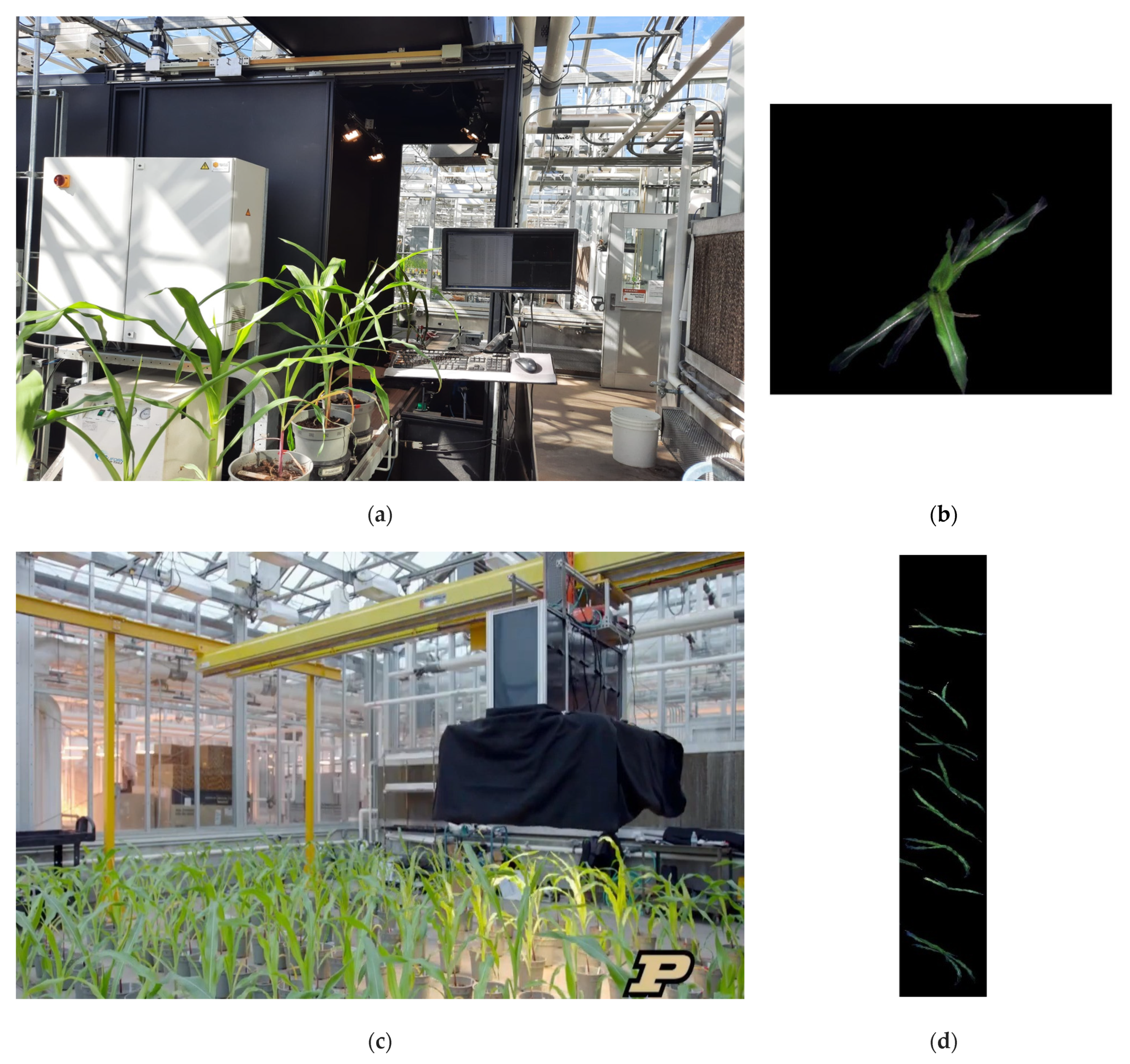
In this study, we used two different hyperspectral imaging systems (Figure 1) to collect the imaging data (referred to as facility 1 and 2 hereafter). Facility 1 consisted of a hyperspectral imaging tower with an automated plant carrier platform and a lighting module (Figure 1a). Images of the individual plants (Figure 1b) were acquired in the absence of ambient light using an MSV-500 pushbroom-style hyperspectral camera (Middleton Spectral Vision, Middleton, WI, USA) encompassing a spectral range of 370 to 1030 nm. Four studio halogen lamps were used for illuminating the plant samples. Complete details about facility 1 can be seen in [24]. Facility 2 contained an automated overhead gantry system for image acquisition (Figure 1c). The plants were arranged on the greenhouse floor in rows and the Specim® FX10e VNIR hyperspectral camera covering a 397–1005 nm region (Specim® spectral imaging Ltd., Oulu, Finland) was flown over the plant rows for image acquisition with the help of the gantry. In contrast to facility 1, hyperspectral images of entire rows (multiple plants per row) were acquired in the ambient lighting (Figure 1d). In addition of using the different cameras and imaging environment, both facilities used different imaging parameters (frame rate, exposure time, spatial and spectral binning) the details of which can be found in [6].
The hyperspectral images from both facilities were calibrated using white boards to remove illumination variations and the sensor’s dark noise. To segment out the plant samples from the background, a convolutional segmentation algorithm mentioned in [9,25] was used. As the hyperspectral images from facility 2 contained multiple plants, therefore, a bounding box scheme mentioned in [26] was used to locate and extract the individual plant hypercubes. The mean spectrum was extracted from the hypercube of an individual plant. From both facilities, the spectral data in the range of 450 nm to 975 nm was retained for further processing.
2.2. Experimental Design and Plant Materials
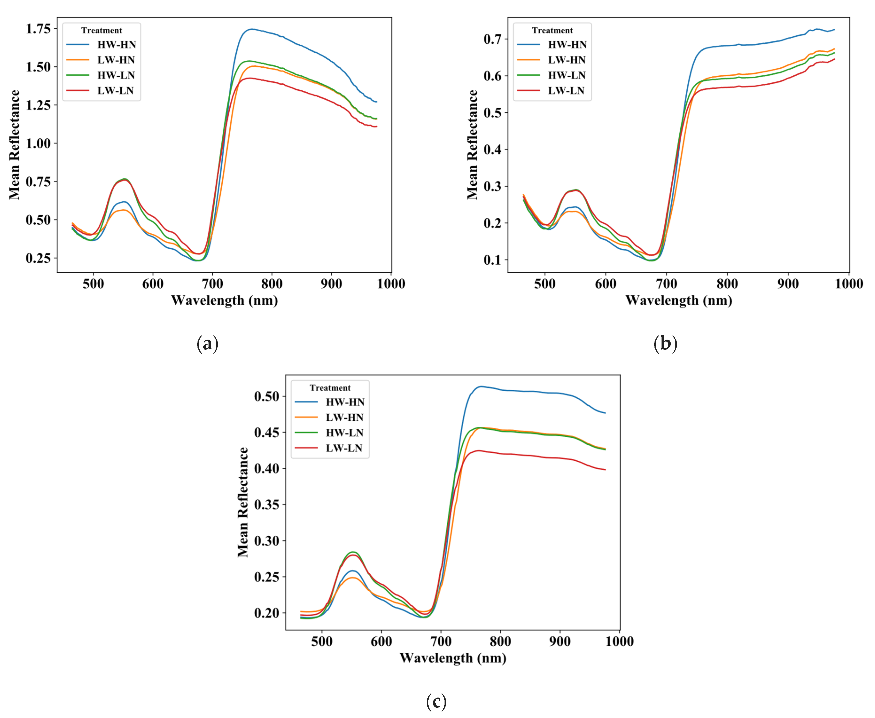
To transfer the calibration models across HTPP facilities, a transfer dataset consisting of the 60 hybrid (B73xMo17) maize plants (Zea mays L.) grown in the Purdue Lilly Green House Facility (40°25′16.2″N, 86°54′53.0″W, https://ag.purdue.edu/LillyGreenhouse/Pages/home.aspx; date accessed: 23 November 2021) was collected. Each plant was treated with one of the two nitrogen treatments, 200 ppm for high nitrogen (HN) and 25 ppm for low nitrogen (LN). In addition to nitrogen, plants were subjected to two water treatments (high water: HW and low water: LW). The water stress was established at V6 growth stage by stopping the water supply for the LW plant samples, while the HW samples were irrigated with sufficient water each day [6]. The imaging in facility 1 was performed two times (at exposure settings of 6 ms and 3 ms, individually) and plants were later imaged in facility 2. In facility 1, white reference panels imaged at 2 ms and 3 ms were used to calibrate the plant samples imaged at 6 ms and 3 ms, respectively. We intentionally selected the exposure time of 2 ms for white panels and 6 ms for the plant samples to introduce nonlinear additive and multiplicative effects in the plant spectra (Figure 2a). The selection of 3 ms as an exposure time for both white panels and plant samples was done to create the differences in imaging/experimental conditions (Figure 2b). Plant samples and white panels were imaged together in facility 2 at exposure settings of 17 ms (Figure 2c).
The second dataset in this study was a calibration dataset containing 200 plants subjected to various water and nitrogen treatments. The plants were imaged only in facility 1 at 6 ms exposure settings and were referenced using a white panel imaged at 2 ms exposure time. For the external evaluation of calibration transfer, we collected a test dataset by imaging the plants (n = 68) in two greenhouse facilities using the same exposure time and imaging parameters as the transfer data. Test plants were subjected to two (HW and LW) water treatments and a nitrogen treatment similar to the transfer data. After imaging, the tissue samples from plants were harvested to collect the nitrogen content and RWC ground truth data. The complete details about these experiments and imaging can be seen in [6].
2.3. Common Latent Space Search
2.3.1. Notations
In this study, the calibration data imaged at 6 ms was used as the master [Xm (nm × p), Y(nm × 1)], while the transfer data imaged in facility 1 at 3 ms [Xs1 (ns × p), Y(ns × 1)] and facility 2 [Xs2 (ns × p), Y(ns × 1)] was used as slave–1 and slave–2, respectively, where nm = 200, ns = 60 are the number of master and slave samples and p denotes the spectral bands. Here, X is the spectral matrix of master or slave datasets, and Y is the corresponding response variable (RWC or N). As the number of spectral bands (p) and spectral resolution were different between the master and facility 2, therefore, we first aligned the slave–2 data by finding its wavelengths that were nearest to the master spectra [6]. This alignment yielded few repeated wavelengths due to the relatively smaller number of bands compared to the master data. These repeated wavelengths were filled by using linear interpolation [16,27]. After the alignment procedure, the slave–2 spectral data have the same number of bands (p) as the master spectra.
2.3.2. Transfer Component Analysis (TCA)
Transfer component analysis extracts a latent representation (features/components) common to both master and slave data in a way that when data from two spectral matrices are projected onto this subspace, the discrepancies between the distributions of the data can be reduced [28]. Let P(Xm) and Q(Xs) be the marginal distributions of the master and slave spectra, respectively, then, the distance between two marginal distributions based on the reproducing kernel Hilbert space (RKHS) can be defined by maximum mean discrepancy (MMD) [29] as in Equation (1).
where UH is a universal RKHS [30], is a nonlinear transformation function, and are the master and slave spectra transformed to RKHS by , respectively. As it is difficult to directly solve for the by minimizing Equation (1) [28], TCA used a kernel trick (i.e., ) to get the kernel matrix (K) (Equation (2)), which can then be used to compute the distance using Equation (3).
where K is the kernel matrix of size (nm + ns) × (nm + ns), ,, are the kernel matrices obtained by applying the kernel (k) on master, slave, across master–slave spectra, respectively, and L is given by Equation (4). In order to find the latent representation, TCA used a matrix for transforming the K to low-rank l-dimensional space (W) with l indicating the transfer components (TCs) common across master–slave spectra. Using the transformed K matrix, the distance represented by Equation (3) can be rewritten as Equation (6). In addition to minimizing the distance between master and slave distributions, an additional regularization term was added to preserve the variance of the data. The objective function thus becomes Equation (7). The solution of W can finally be the l-leading eigenvectors of , where l is the number of extracted transfer components (Equation (8)).
where I is the identity matrix, is the trade-off factor that was manually adjusted, and H is the centering matrix [28]. Finally, the master () and slave () data can be converted to transfer components using Equation (9).
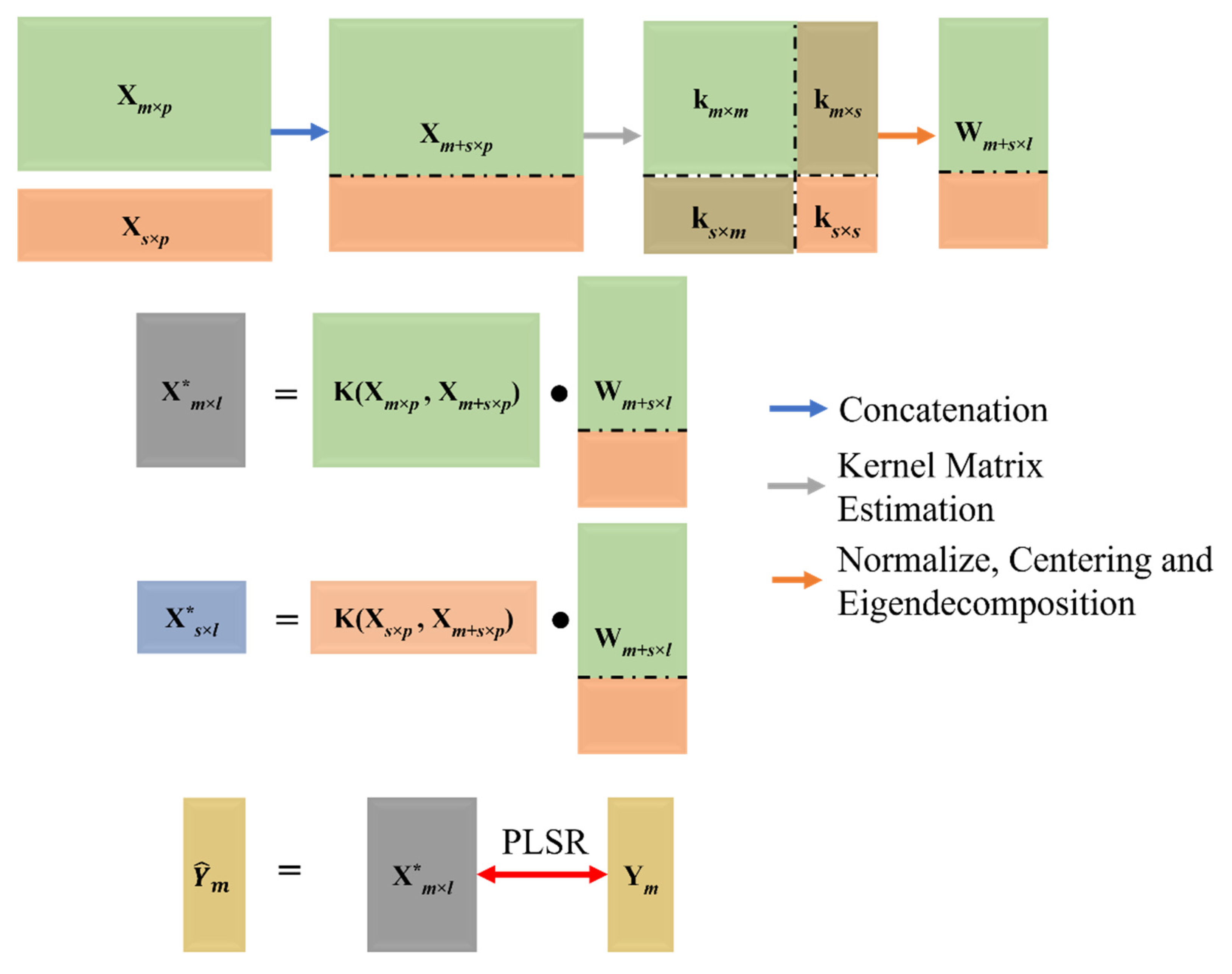
In this study, we investigated a linear kernel for estimating the K matrix since all other methods (c-PCA, di-PLSR) reported here were essentially linear. From both master and slave data, 40 TCs were extracted. A schematic showing the complete TCA algorithm is presented in Figure 3.
2.3.3. Combined Principal Component Analysis (c-PCA)
To extract the components common across master and slave spectra, principal component analysis (PCA) was performed on the combined master and slave spectra ); therefore, called combined PCA (c-PCA). The common principal components (PCs) from the Xm together with the master response (Ym) were used to develop the calibration model. Similar to TCA, 40 PCs were from both master and slave datasets.
2.3.4. Domain Invariant Partial Least Squares Regression (di-PLSR)
Domain invariant partial least squares regression is an extension of ordinary PLSR to align the master (Xm) and slave (Xs) spectral data in the latent space by minimizing the variances across master–slave spectral data while maximizing the covariance between the Y and Xm [10,31]. The di-PLSR uses a non-linear iterative partial least squares (NIPALS) algorithm to align the master–slave variances by reforming the original objective function for calculating the weight vector (w) as in Equation (10).
where and represent Frobenius norm and across spectra regularization parameter, whereas tm and ts are master and slave data projections (scores) on w. Equation (10) can be expanded as Equation (11).
The nm and ns are the number of samples in the source and slave data, and represents a matrix having all absolute eigenvalues () obtained via eigendecomposition (Equation (12)).
The K represents an eigenvector matrix of differences in the spectral data source-specific covariance matrices [31]. The first term in Equation (10) is the standard NIPLAS function, which can be minimized using a least-squares approach to find the w that can result in maximum covariance between Xm and Y. The other term in Equation (10) denotes an upper bound on the absolute difference in master and slave variance in direction of w [31]. The least-squares solution of Equation (11) can provide the w as in Equation (13).
Similar to NIPLAS, the weight vector needs to be normalized. The master (tm) and slave (ts) projections (scores) on w can be computed as Equation (14).
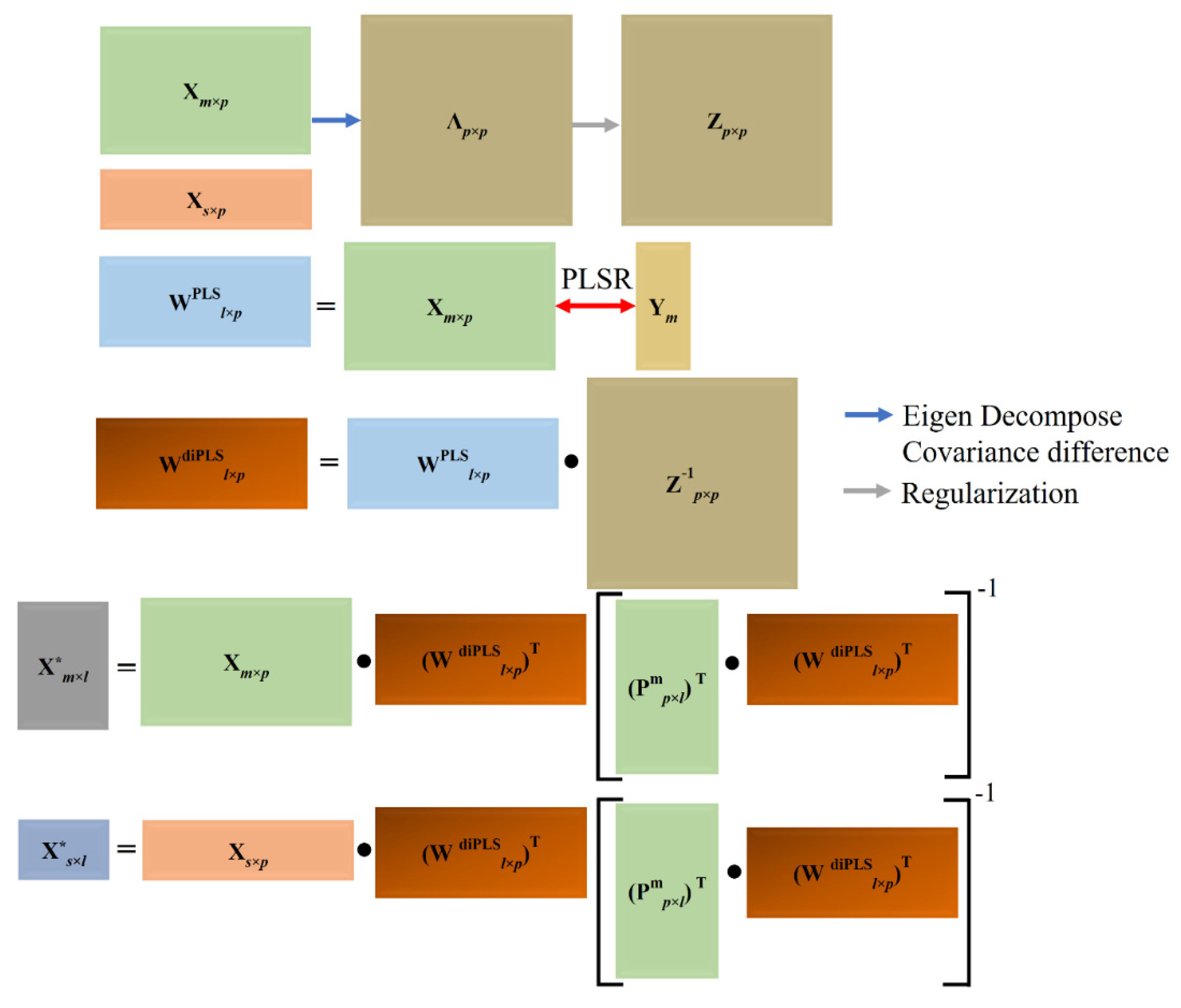
The di-PLSR performs the orthogonalization (Equation (15)) similar to PLSR to remove the variations in the spectral data (Xm or Xs), which have already been explained by the current latent variable (LV). A schematic showing the high-level information of di-PLSR can be seen in Figure 4. The remainder of the di-PLSR algorithm is the same as standard PLSR [31]. For this study, the regularization parameter was adjusted for each LV as per the heuristics defined in [31]. Briefly, these heuristics adjusted so that both terms in Equation (10) have equal weights. To finetune the number of LVs, we used 5–fold CV with the lowest RMSEcv indicting the optimal number of LVs.
2.4. Calibration Models
For methods extracting components (TCA and PCA), PLSR was applied to establish the calibration models between the extracted components and response variable. The spectral data were preprocessed using , mean scatter correction (MSC), and mean centering (MC) [9] before the common latent space exploration via all these calibration transfer methods. Before developing the models, both response variables (RWC and N) were scaled to unit variance and zero-centered using their standard deviations and means, respectively. In addition to the transferred models, two PLSR (RWC and N) models were developed using master data only (200 plants imaged in facility 1 at 6 ms and referenced with a 2 ms white reference) to predict RWC and N (called master models hereafter). These models were used to obtain the predictions of plants imaged with 6 ms and referenced with 2 ms exposure in facility 1 for two (transfer and test) datasets. These predictions (called master predictions hereafter) were used to assess the performance of different transferred models.
3. Results
3.1. Comparison of Calibration Transfer Methods for RWC
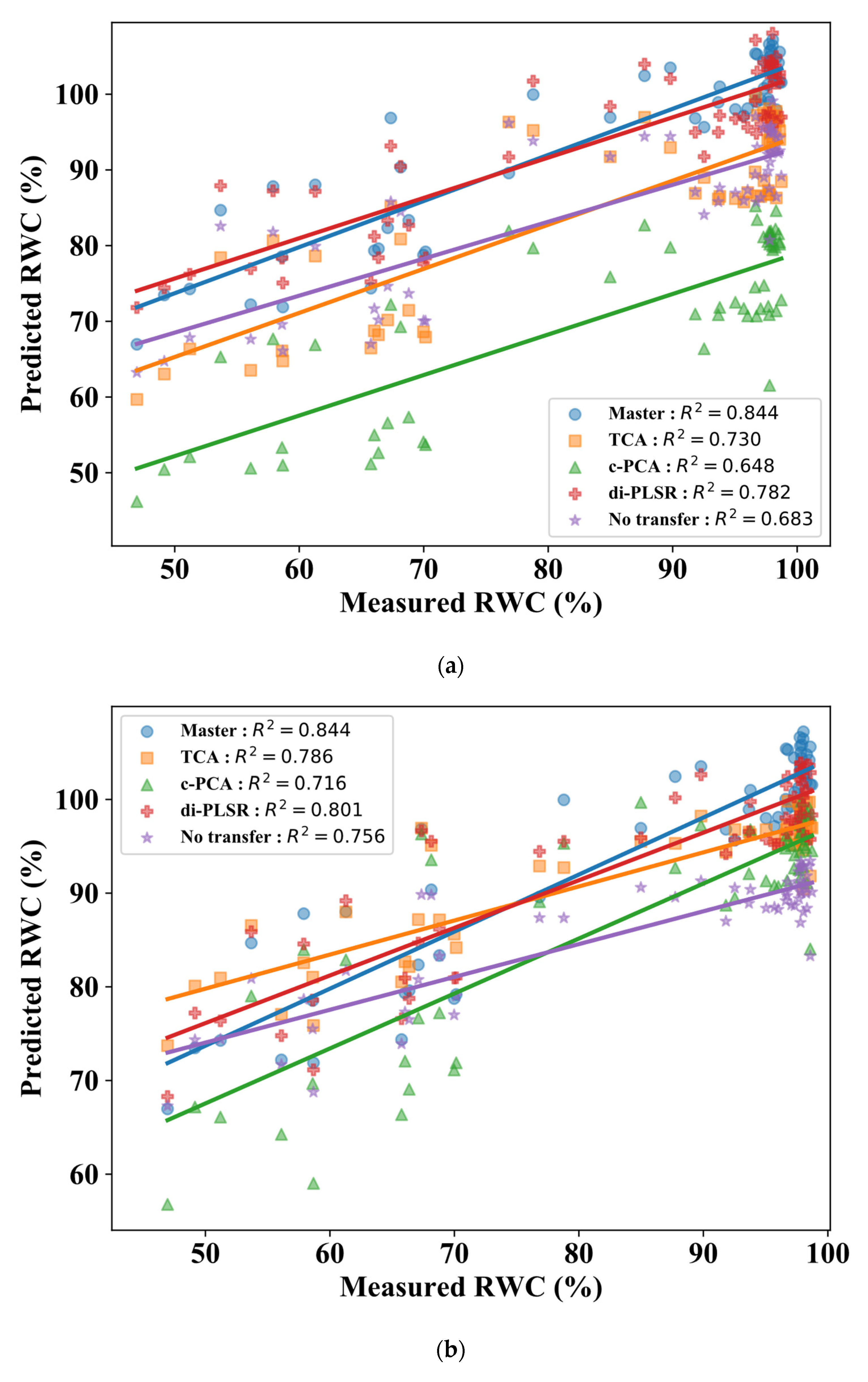
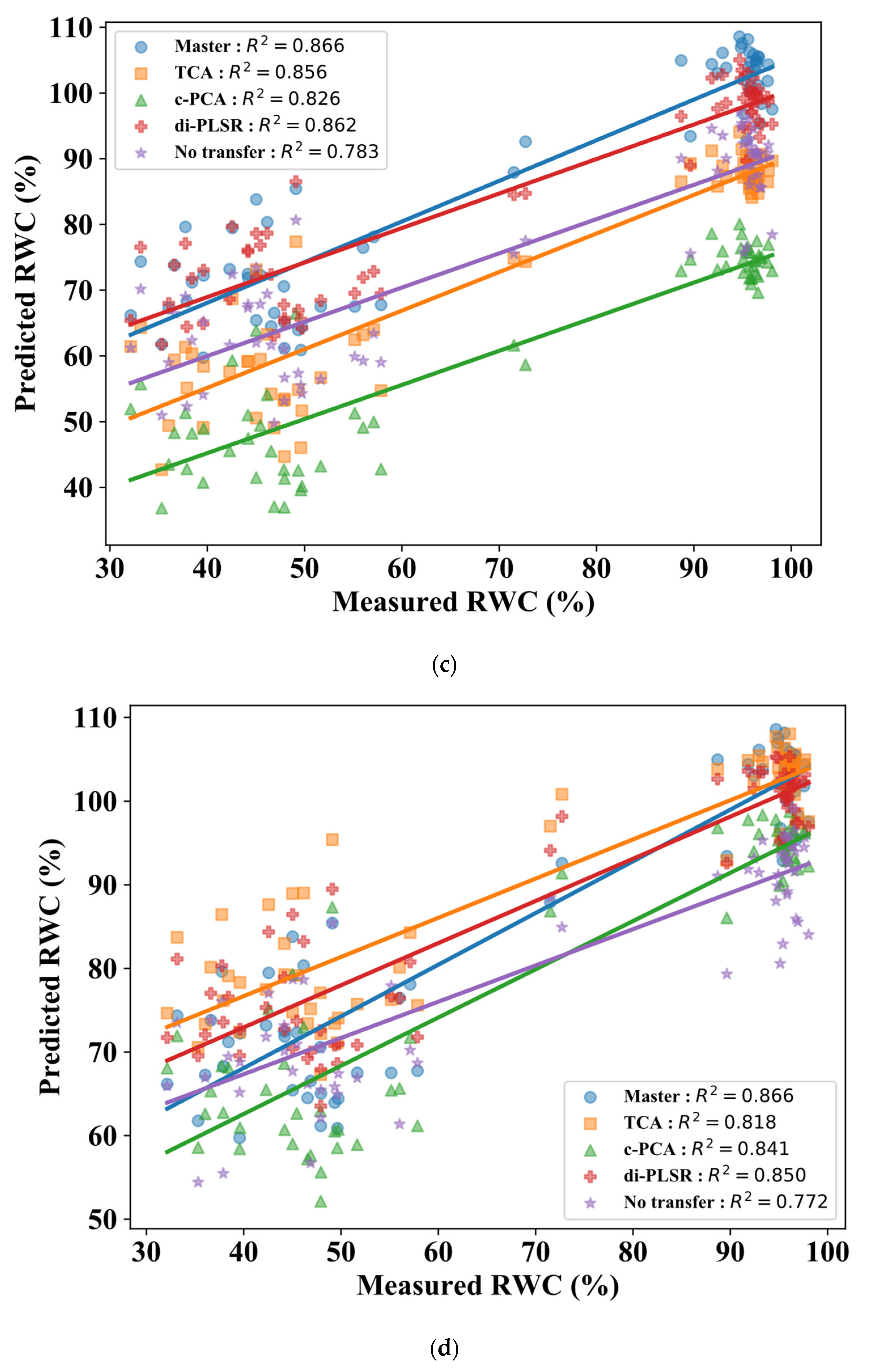
Figure 5 and Table 1 show the results of calibration transfer methods adopted in this study for RWC predictions. Applying the master RWC calibration model on master spectra achieved a coefficient of determination (R2) of 0.844, which was dropped to 0.683 and 0.756 when the same model was used to obtain the predictions for slave–1 and slave–2 validation data, respectively (Figure 5a,b: blue circles vs. purple stars). Similarly, for the test dataset, the R2 was reduced from 0.866 to 0.783 and 0.772 for slave–1 and slave–2 data (Figure 5c,d: blue circles vs. purple stars). Using a master PLSR calibration model on raw slave spectra (no calibration transfer) showed the large discrepancies between master and slave (slave–1: RMSEv = 10.183% and slave–2: RMSEv = 10.083%) predictions (Table 1).
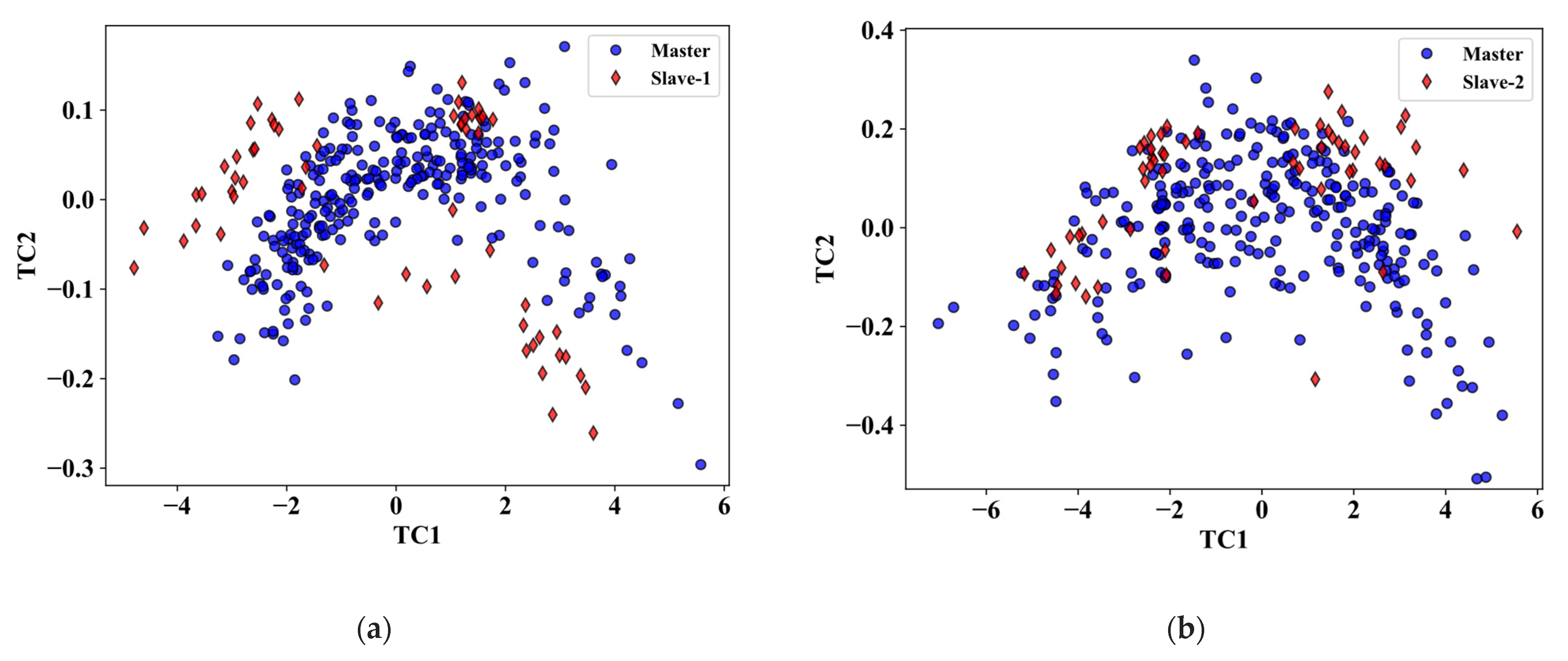
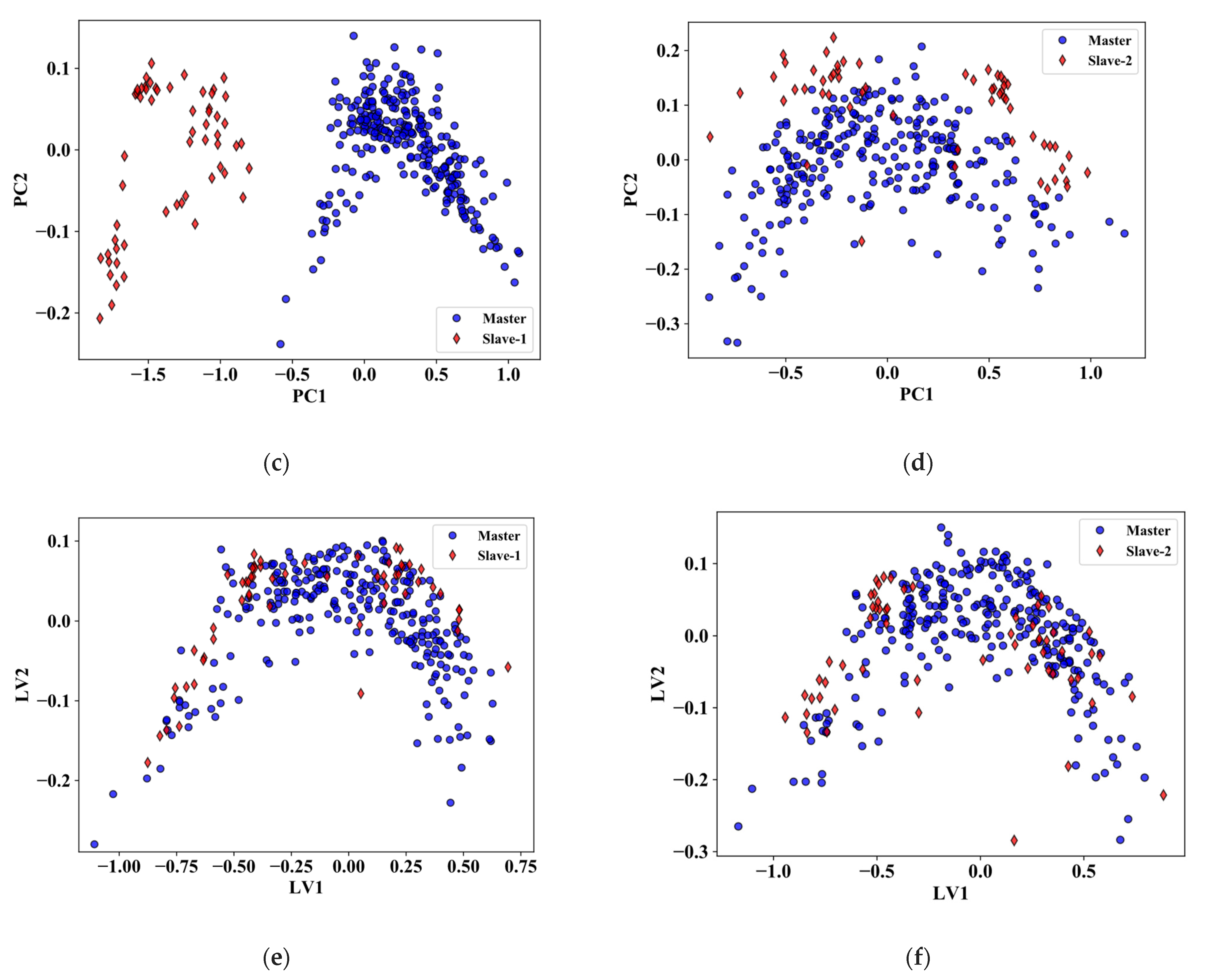
Adopting di-PLSR for calibration transfer relatively reduced the error in RWC predictions compared to master data for both slave–1 and slave–2 datasets. In the case of slave–1 validation and test data, the di-PLSR decreased RMSE by 74.49% and 64.96%, respectively. For slave–2 validation and test data, the RMSE was decreased by 72.56% and 56.38%, respectively. Subjective evaluation via Figure 5 (red crosses) indicated that the di-PLSR regression line was fairly closely aligned with the master regression line for all datasets, which significantly helped to recover the R2 value lost by non-transferred predictions. The TCA and c-PCA, however, reduced the error only for slave–2 data, while for slave–1, they degraded the predictions. Figure 5a,c (orange square) showed that the TCA was not able to reduce the offset compared to master predictions and the regression line was roughly similar to non-transferred predictions with little improvements. These improvements, though, increased the R2 but were not instrumental to reduce the discrepancies (RMSE). The visual evaluation indicated that the offset between master and c-PCA predictions turned out to be even larger as compared to the non-transferred case (Figure 5a,c: green triangles). In contrast, TCA and c-PCA predictions for slave–2 were closer to the master predictions and, therefore, have relatively better R2, RMSE, and MAPE (Table 1 and Figure 5b,d). The improved performance of TCA and c-PCA for slave–2 data can be due to the relatively better alignment of master and slave–2 spectra in latent space compared with slave–1 (Figure 6a–d). The c-PCA on the other hand was not able to extract the latent space representation common to both master and slave–1 (Figure 6c). Although TCA and c-PCA improved results for slave–2, their performance was not at par with di-PLSR. The improved results of di-PLSR can be due to the better latent space alignment between master and slave datasets (Figure 6e,f). These results showed the ability of di-PLSR to perform the RWC model calibration transfer.
3.2. Comparison of Calibration Transfer Methods for Nitrogen
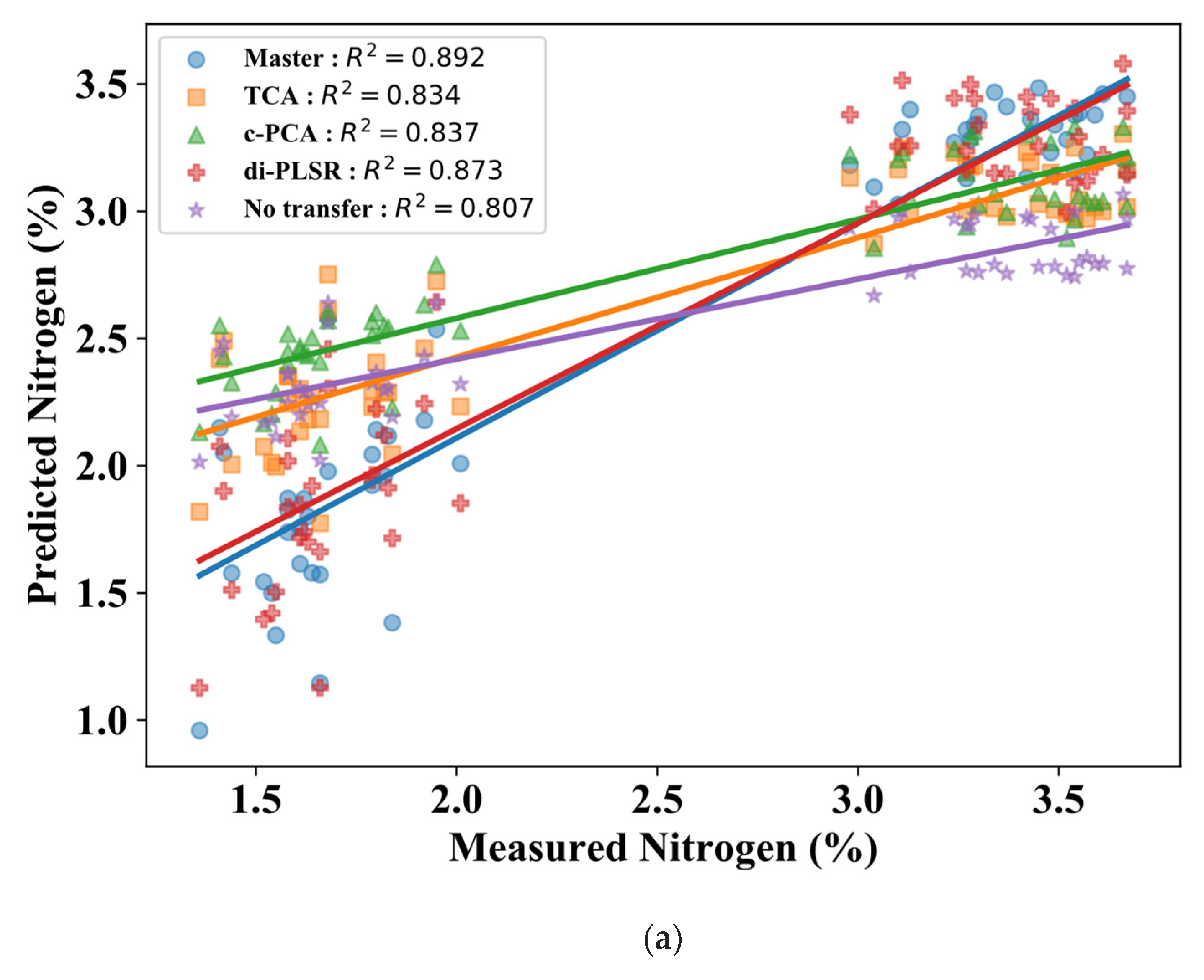
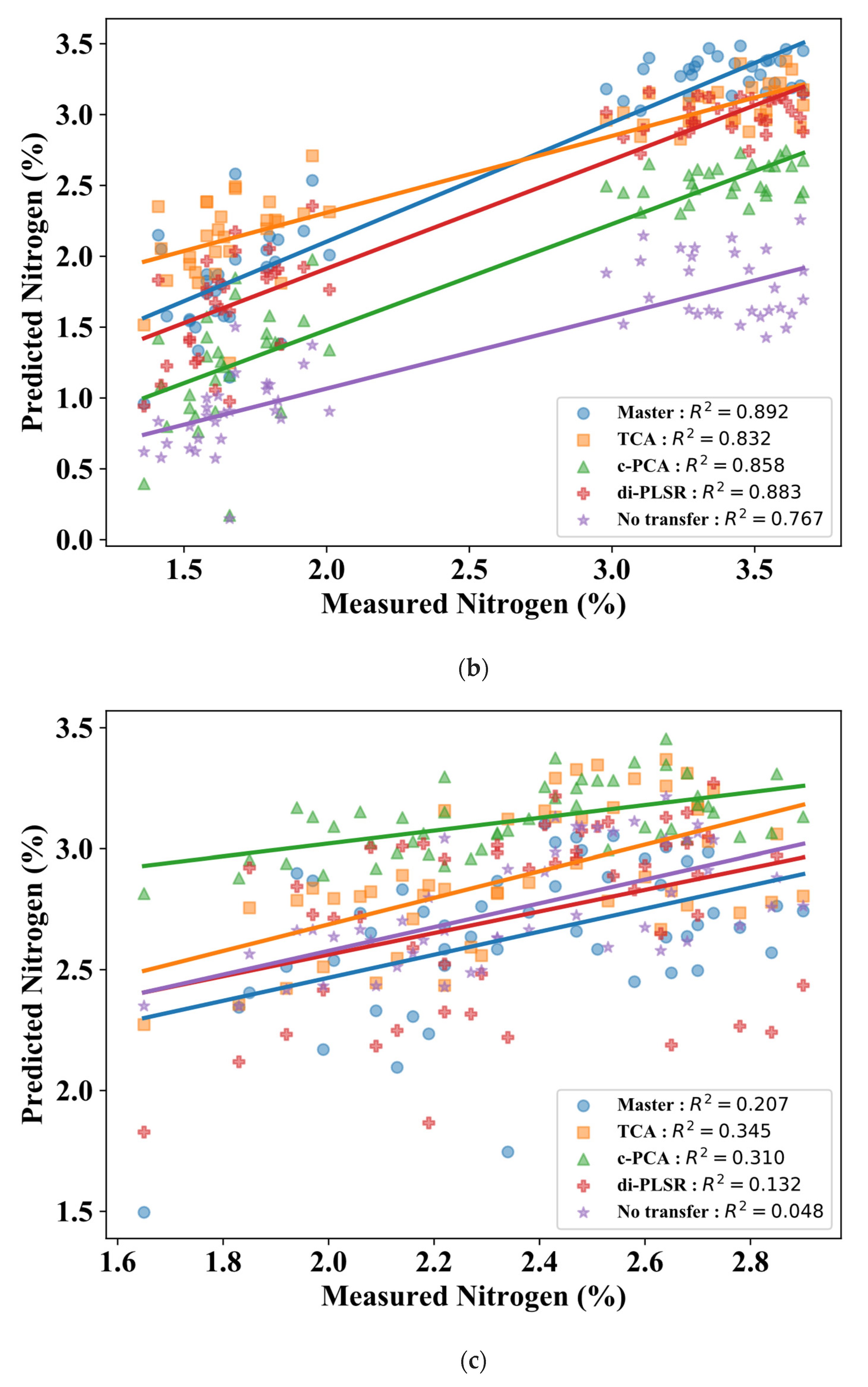
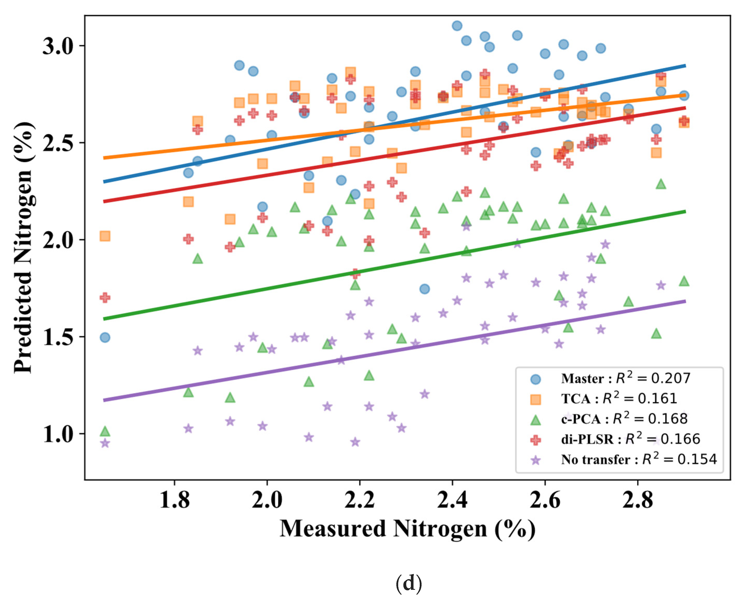
Figure 7 and Table 2 show the results of calibration transfer methods adopted in this study for nitrogen predictions. Since all plant samples for test data were treated with the same nitrogen level, we considered only RMSE and MAPE for comparing the performance of different calibration transfer techniques. When no calibration transfer was performed, the R2 for nitrogen was dropped from 0.892 to 0.807 and 0.767 for slave–1 and slave–2 validation data, respectively (Figure 7a,b: blue circles vs. purple stars). Without any calibration transfer, the RMSEv and prediction root mean square error (RMSEp) for the slave–1 dataset were 0.511% and 0.493%, respectively. For slave–2 spectra, the corresponding statistics were 1.276% and 1.212%, respectively (Table 2). In contrast to slave–1, the RMSEv and RMSEp for slave–2 were relatively high due to the larger offset between master and slave–2 predictions (Figure 7b,d). The calibration transfer via di-PLSR reduced the RMSEv to 0.193% and 0.297%, while RMSEp to 0.277% and 0.286% for slave–1 and slave–2 data, respectively. Figure 7 (red crosses) shows the improvement obtained by di-PLSR nitrogen predictions for both slave–1 and slave–2 data and, therefore, recovered the R2 value lost by non-transferred predictions. Similar to RWC, the TCA reduced the RMSEv and RMSEp (Table 2) and improved the R2 (Figure 7b,d) of nitrogen predictions for slave–2 data. In contrast to the RWC, the TCA improved the predictions of the nitrogen model for the slave–1 data. Subjectively, small improvements in the nitrogen predictions can also be seen in Figure 7a,c (orange squares). Although the TCA reduced RMSE, this error reduction for slave–1 (22.90% and 17.45% for validation and test, respectively) was relatively less compared to the slave–2 (75.47% and 76.40% for validation and test, respectively). The c-PCA for nitrogen showed results similar to RWC, i.e., improvement in the slave–2 and degradation in the slave–1 predictions (Figure 7a–d: green triangles). The degradation was due to the failure of c-PCA to extract the latent space common to both master and slave–1 data as mentioned earlier. These results indicated that calibration models can be transferred to different HTPP facilities equipped with hyperspectral cameras using di-PLSR.
4. Discussion
The plant phenotypic features prediction models developed using spectral reflectance data from HTPP systems are usually facility-specific. The calibration models developed in one facility often fail to perform reliably when applied on a spectrum collected from a new HTPP facility or under different imaging/experimental conditions. Therefore, the transfer of these calibration models is essential for ubiquitous application of HTPP systems. This work reported the application of TCA, c-PCA, and di-PLSR to transfer the calibration models by learning the underlying common latent space. The proposed di-PLSR improved the RWC and nitrogen prediction performances without requiring the standard plant samples when challenged with imaging conditions variations (slave–1) and a new HTPP facility (slave–2).
When transferring the RWC calibration model, TCA and c-PCA improved the predictions for the new HTPP facility, while for an existing facility with different experimental conditions, these methods degraded the performance. These results were in contrast to [32], where TCA showed an improvement of 11.84% in the R2 for experimental condition change (fruit temperature changes) and 7.32% for a new instrument. The contrasting results of our study compared to [32] could be due to the nature of change in experimental conditions, i.e., fruit temperature change versus the change in exposure settings. Another reason for better results for only slave–2 in our study can be due to the better alignment of master and slave–2 spectra in common latent space extracted by TCA, which helped to reduce the prediction discrepancies. In the case of slave–1, an offset (Figure 6a) between slave–1 and master data was observed along the first transfer component (TC1), which might explain the prediction offset of slave–1 in Figure 5a,c. The c-PCA was not able to extract the latent space representation common to both master and slave–1 (Figure 6c) and, therefore, resulted in poor performance. The discrepancy in the latent space for slave–1 could be due to the inability of TCA and c-PCA to correctly capture the additive reflectance offset or complex multiplicative perturbations in the blue and near-infrared portions, thus varying the spectral shape and slope in these regions (Figure 2) [6]. Shi et al. [33] combined TCA, PCA, and artificial neural networks to predict the compression strength of forest trees using NIR spectra. The study first extracted the common components among two species of hardwood using TCA followed by PCA to further reduce the common features. Finally, the ANN model trained with master data was finetuned using the labeled samples from the slave dataset. The best results were reported when 60% of the samples from slave data were used for finetuning the model. However, in this study, the labels from the slave data were never used to update the model. For nitrogen model transfer, the results of TCA were contrastingly different than RWC for slave–1 data. The better performance of TCA for slave–1 nitrogen predictions compared to RWC can be attributed to the downstream PLSR model that is learning the association between TCA components and response variable (RWC or N). Analyzing the regression coefficients (β) of RWC and nitrogen models indicated that the nitrogen model has given relatively less weight to the TC1 compared to RWC and, therefore, might be relatively less impacted by the master and slave–1 offset along the TC1. Mishra et al. [34] used the di-PLSR to adapt a calibration model developed on one spectrometer to another instrument for predicting the dry matter content of olive fruit. The results showed that di-PLSR can considerably improve the model performance when tested on the new instrument. While the study involved two different spectrometers, both of them were from the same manufacturer with a difference being produced under different batches [35]. In comparison, our study applied TCA, c-PCA, and di-PLSR to an unexplored area of HTPP facilities with relatively more sources of variations including sensor type, spectrograph, lens system, spatial resolution, spectral resolution, the field of view, bit-depth, frame rate, and exposure time [6]. These facilities also used hyperspectral cameras instead of spectrometers. In addition to the imaging system variations, the two HTPP facilities have completely different lighting sources (artificial versus ambient lighting). Our study clearly showed that even in the presence of larger sources of variations (imaging system + lighting conditions), di-PLSR can be successfully used to transfer the calibration models across different HTPP systems. Persistent to results of this research, the study conducted by [31] showed the better performance of the di-PLSR compared to the TCA. In contrast to the methods reported by [6,36,37], our proposed techniques relax the condition of imaging the same plants in two HTPP facilities.
5. Conclusions
Transfer of calibration models is essential for ubiquitous applications of HTPP systems equipped with hyperspectral cameras. An existing multivariate model can potentially lead to poor predictions because of the variations in instrumental response over time, the difference in experimental conditions, the difference between hyperspectral cameras, or image acquisition in different imaging facilities. In the current work, TCA, c-PCA, and di-PLSR were proposed to perform calibration transfer via learning an intermediate latent space common between master and slave data. The main advantage of the suggested techniques is to avoid the need of imaging the same standard samples in different phenotyping facilities for calibration transfer as in the case of [6]. The suggested methods were tested to transfer the RWC and N calibration models. The quantitative analysis showed that the di-PLSR alleviated the perturbations inherited in the spectral data for both RWC and N predictions. The di-PLSR reduced the RWC RMSEv from 10.183% to 2.598% for slave–1 and from 10.083% to 2.767% for slave–2 data. Similarly, for nitrogen, the RMSEv was reduced from 0.511% to 0.193% for slave–1 and from 1.276% to 0.297% for slave–2. Based on the performance evaluation, it can be concluded that the di-PLSR can alleviate the requirement of developing a new calibration model for every phenotyping facility or to resort to the spectral space adjustment using the standard samples.
Author Contributions
Conceptualization, T.U.R. and J.J.; methodology, T.U.R.; software, T.U.R.; validation, T.U.R., L.Z. and D.M.; formal analysis, T.U.R.; investigation, T.U.R. and L.Z.; resources, J.J.; data curation, L.Z.; writing—original draft preparation, T.U.R.; writing—review and editing, D.M. and J.J.; visualization, D.M.; supervision, J.J.; project administration, J.J.; funding acquisition, J.J. All authors have read and agreed to the published version of the manuscript.
Funding
This research was funded by Purdue University.
Institutional Review Board Statement
Not applicable.
Informed Consent Statement
Not applicable.
Data Availability Statement
The data presented in this study are available on request from the corresponding author. The data are not publicly available due to confidentiality.
Acknowledgments
This work was sponsored by Agricultural and Biological Engineering at Purdue University. The authors appreciate the help and assistance of Andrew Linvill (Research Geneticist, Department of Agronomy at Purdue University) and Meng-Yang Lin (Student, Department of Agronomy at Purdue University) during ground truth collection and cultivation of plants.
Conflicts of Interest
The authors declare no conflict of interest.
References
- Fiorani, F.; Schurr, U. Future Scenarios for Plant Phenotyping. Annu. Rev. Plant Biol. 2013, 64, 267–291. [Google Scholar] [CrossRef] [Green Version]
- Walter, A.; Liebisch, F.; Hund, A. Plant Phenotyping: From Bean Weighing to Image Analysis. Plant Methods 2015, 11, 14. [Google Scholar] [CrossRef] [Green Version]
- Costa, C.; Schurr, U.; Loreto, F.; Menesatti, P.; Carpentier, S. Plant Phenotyping Research Trends, a Science Mapping Approach. Front. Plant Sci. 2019, 9, 1933. [Google Scholar] [CrossRef] [Green Version]
- Roitsch, T.; Cabrera-Bosquet, L.; Fournier, A.; Ghamkhar, K.; Jiménez-Berni, J.; Pinto, F.; Ober, E.S. Review: New Sensors and Data-Driven Approaches—A Path to next Generation Phenomics. Plant Sci. 2019, 282, 2–10. [Google Scholar] [CrossRef]
- das Choudhury, S.; Samal, A.; Awada, T. Leveraging Image Analysis for High-Throughput Plant Phenotyping. Front. Plant Sci. 2019, 10, 508. [Google Scholar] [CrossRef]
- Rehman, T.U.; Zhang, L.; Ma, D.; Wang, L.; Jin, J. Calibration Transfer across Multiple Hyperspectral Imaging-Based Plant Phenotyping Systems: I—Spectral Space Adjustment. Comput. Electron. Agric. 2020, 176, 105685. [Google Scholar] [CrossRef]
- Ge, Y.; Atefi, A.; Zhang, H.; Miao, C.; Ramamurthy, R.K.; Sigmon, B.; Yang, J.; Schnable, J.C. High-Throughput Analysis of Leaf Physiological and Chemical Traits with VIS-NIR-SWIR Spectroscopy: A Case Study with a Maize Diversity Panel. Plant Methods 2019, 15, 66. [Google Scholar] [CrossRef] [Green Version]
- Zhang, L.; Rao, Z.; Ji, H. NIR Hyperspectral Imaging Technology Combined with Multivariate Methods to Study the Residues of Different Concentrations of Omethoate on Wheat Grain Surface. Sensors 2019, 19, 3147. [Google Scholar] [CrossRef] [PubMed] [Green Version]
- Rehman, T.U.; Ma, D.; Wang, L.; Zhang, L.; Jin, J. Predictive Spectral Analysis Using an End-to-End Deep Model from Hyperspectral Images for High-Throughput Plant Phenotyping. Comput. Electron. Agric. 2020, 177, 105713. [Google Scholar] [CrossRef]
- Nikzad-Langerodi, R.; Zellinger, W.; Lughofer, E.; Saminger-Platz, S. Domain-Invariant Partial-Least-Squares Regression. Anal. Chem. 2018, 90, 6693–6701. [Google Scholar] [CrossRef] [PubMed]
- Zhang, F.; Zhang, R.; Ge, J.; Chen, W.; Yang, W.; Du, Y. Calibration Transfer Based on the Weight Matrix (CTWM) of PLS for near Infrared (NIR) Spectral Analysis. Anal. Methods 2018, 10, 2169–2179. [Google Scholar] [CrossRef]
- Li, X.Y.; Ren, G.X.; Fan, P.P.; Liu, Y.; Sun, Z.L.; Hou, G.L.; Lv, M.R. Study on the Calibration Transfer of Soil Nutrient Concentration from the Hyperspectral Camera to the Normal Spectrometer. J. Spectrosc. 2020, 2020, 8137142. [Google Scholar] [CrossRef]
- Murphy, R.J.; Schneider, S.; Monteiro, S.T. Consistency of Measurements of Wavelength Position from Hyperspectral Imagery: Use of the Ferric Iron Crystal Field Absorption at ~900 Nm as an Indicator of Mineralogy. IEEE Trans. Geosci. Remote Sens. 2014, 52, 2843–2857. [Google Scholar] [CrossRef]
- Buddenbaum, H.; Watt, M.S.; Scholten, R.C.; Hill, J. Preprocessing Ground-Based Visible/near Infrared Imaging Spectroscopy Data Affected by Smile Effects. Sensors 2019, 19, 1543. [Google Scholar] [CrossRef] [PubMed] [Green Version]
- Fearn, T. Standardisation and Calibration Transfer for near Infrared Instruments: A Review. J. Near Infrared Spectrosc. 2001, 9, 229–244. [Google Scholar] [CrossRef]
- Alamar, M.C.; Bobelyn, E.; Lammertyn, J.; Nicolaï, B.M.; Moltó, E. Calibration Transfer between NIR Diode Array and FT-NIR Spectrophotometers for Measuring the Soluble Solids Contents of Apple. Postharvest Biol. Technol. 2007, 45, 38–45. [Google Scholar] [CrossRef]
- Ji, W.; Viscarra Rossel, R.A.; Shi, Z. Improved Estimates of Organic Carbon Using Proximally Sensed Vis-NIR Spectra Corrected by Piecewise Direct Standardization. Eur. J. Soil Sci. 2015, 66, 670–678. [Google Scholar] [CrossRef]
- Li, X.; Cai, W.; Shao, X. Correcting Multivariate Calibration Model for near Infrared Spectral Analysis without Using Standard Samples. J. Near Infrared Spectrosc. 2015, 23, 285–291. [Google Scholar] [CrossRef]
- Pu, Y.Y.; Sun, D.W.; Riccioli, C.; Buccheri, M.; Grassi, M.; Cattaneo, T.M.P.; Gowen, A. Calibration Transfer from Micro NIR Spectrometer to Hyperspectral Imaging: A Case Study on Predicting Soluble Solids Content of Bananito Fruit (Musa Acuminata). Food Anal. Methods 2018, 11, 1021–1033. [Google Scholar] [CrossRef]
- Workman, J.J. A Review of Calibration Transfer Practices and Instrument Differences in Spectroscopy. Appl. Spectrosc. 2018, 72, 340–365. [Google Scholar] [CrossRef]
- Fan, S.; Li, J.; Xia, Y.; Tian, X.; Guo, Z.; Huang, W. Long-Term Evaluation of Soluble Solids Content of Apples with Biological Variability by Using near-Infrared Spectroscopy and Calibration Transfer Method. Postharvest Biol. Technol. 2019, 151, 79–87. [Google Scholar] [CrossRef]
- Du, W.; Chen, Z.P.; Zhong, L.J.; Wang, S.X.; Yu, R.Q.; Nordon, A.; Littlejohn, D.; Holden, M. Maintaining the Predictive Abilities of Multivariate Calibration Models by Spectral Space Transformation. Anal. Chim. Acta 2011, 690, 64–70. [Google Scholar] [CrossRef]
- Folch-Fortuny, A.; Vitale, R.; de Noord, O.E.; Ferrer, A. Calibration Transfer between NIR Spectrometers: New Proposals and a Comparative Study. J. Chemom. 2017, 31, e2874. [Google Scholar] [CrossRef]
- Ma, D.; Carpenter, N.; Amatya, S.; Maki, H.; Wang, L.; Zhang, L.; Neeno, S.; Tuinstra, M.R.; Jin, J. Removal of Greenhouse Microclimate Heterogeneity with Conveyor System for Indoor Phenotyping. Comput. Electron. Agric. 2019, 166, 104979. [Google Scholar] [CrossRef]
- Zhang, L.; Maki, H.; Ma, D.; Sánchez-Gallego, J.A.; Mickelbart, M.V.; Wang, L.; Rehman, T.U.; Jin, J. Optimized Angles of the Swing Hyperspectral Imaging System for Single Corn Plant. Comput. Electron. Agric. 2019, 156, 349–359. [Google Scholar] [CrossRef]
- Rehman, T.U.; Zhang, L.; Wang, L.; Ma, D.; Maki, H.; Sánchez-Gallego, J.A.; Mickelbart, M.V.; Jin, J. Automated Leaf Movement Tracking in Time-Lapse Imaging for Plant Phenotyping. Comput. Electron. Agric. 2020, 175, 105623. [Google Scholar] [CrossRef]
- Bin, J.; Li, X.; Fan, W.; Zhou, J.H.; Wang, C.W. Calibration Transfer of Near-Infrared Spectroscopy by Canonical Correlation Analysis Coupled with Wavelet Transform. Analyst 2017, 142, 2229–2238. [Google Scholar] [CrossRef] [PubMed]
- Pan, S.J.; Tsang, I.W.; Kwok, J.T.; Yang, Q. Domain Adaptation via Transfer Component Analysis. IEEE Trans. Neural Netw. 2011, 22, 199–210. [Google Scholar] [CrossRef] [PubMed] [Green Version]
- Borgwardt, K.M.; Gretton, A.; Rasch, M.J.; Kriegel, H.P.; Schölkopf, B.; Smola, A.J. Integrating Structured Biological Data by Kernel Maximum Mean Discrepancy. Bioinformatics 2006, 22, e49–e57. [Google Scholar] [CrossRef] [PubMed] [Green Version]
- Steinwart, I. On the Influence of the Kernel on the Consistency of Support Vector Machines. J. Mach. Learn. Res. 2002, 2, 67–93. [Google Scholar] [CrossRef]
- Nikzad-Langerodi, R.; Zellinger, W.; Saminger-Platz, S.; Moser, B.A. Domain Adaptation for Regression under Beer–Lambert’s Law. Knowl.-Based Syst. 2020, 210, 106447. [Google Scholar] [CrossRef]
- Mishra, P.; Roger, J.M.; Rutledge, D.N.; Woltering, E. Two Standard-Free Approaches to Correct for External Influences on near-Infrared Spectra to Make Models Widely Applicable. Postharvest Biol. Technol. 2020, 170, 111326. [Google Scholar] [CrossRef]
- Shi, G.; Cao, J.; Li, C.; Liang, Y. Compression Strength Prediction of Xylosma Racemosum Using a Transfer Learning System Based on Near-Infrared Spectral Data. J. For. Res. 2020, 31, 1061–1069. [Google Scholar] [CrossRef] [Green Version]
- Mishra, P.; Nikzad-Langerodi, R. Partial Least Square Regression versus Domain Invariant Partial Least Square Regression with Application to Near-Infrared Spectroscopy of Fresh Fruit. Infrared Phys. Technol. 2020, 111, 103547. [Google Scholar] [CrossRef]
- Sun, X.; Subedi, P.; Walker, R.; Walsh, K.B. NIRS Prediction of Dry Matter Content of Single Olive Fruit with Consideration of Variable Sorting for Normalisation Pre-Treatment. Postharvest Biol. Technol. 2020, 163, 111140. [Google Scholar] [CrossRef]
- Li, L.; Jang, X.; Li, B.; Liu, Y. Wavelength Selection Method for Near-Infrared Spectroscopy Based on Standard-Sample Calibration Transfer of Mango and Apple. Comput. Electron. Agric. 2021, 190, 106448. [Google Scholar] [CrossRef]
- Li, X.; Li, Z.; Yang, X.; He, Y. Boosting the Generalization Ability of Vis-NIR-Spectroscopy-Based Regression Models through Dimension Reduction and Transfer Learning. Comput. Electron. Agric. 2021, 186, 106157. [Google Scholar] [CrossRef]
Figure 1.
Two HTPP facilities used for this study: (a) a hyperspectral imaging tower, (b) masked RGB image of a plant, (c) gantry imaging facility, and (d) masked RGB image of multiple plants.
Figure 1.
Two HTPP facilities used for this study: (a) a hyperspectral imaging tower, (b) masked RGB image of a plant, (c) gantry imaging facility, and (d) masked RGB image of multiple plants.

Figure 2.
Mean reflectance profiles of the different treatments: (a) plants imaged in facility 1 with 6 ms exposure, (b) plants imaged in facility 1 with 3 ms exposure, and (c) plants imaged in facility 2.
Figure 2.
Mean reflectance profiles of the different treatments: (a) plants imaged in facility 1 with 6 ms exposure, (b) plants imaged in facility 1 with 3 ms exposure, and (c) plants imaged in facility 2.

Figure 3.
A schematic to illustrate the working principle of TCA (here, m = nm and s = ns).

Figure 4.
A schematic to illustrate the working principle of di-PLSR (here, m = nm and s = ns).

Figure 5.
Measured and predicted RWC using TCA, c-PCA, and di-PLSR calibration transfer approaches: (a) slave–1 validation, (b) slave–2 validation, (c) slave–1 test, and (d) slave–2 test data. Predictions from master data are presented in blue circles, TCA in orange squares, c-PCA in green triangles, di-PLSR in red crosses, and no transfer in purple stars.


Figure 6.
Latent space representations: (a,b) projections of master along with slave–1 and slave–2 data on the first 2 components of TCA, respectively; (c,d) projections of master along slave–1 and slave–2 data on the first 2 components of PCA, respectively; and (e,f) projections of master along with slave–1 and slave–2 data on the first 2 LVs of di-PLSR, respectively.


Figure 7.
Measured and predicted nitrogen using TCA, c-PCA, and di-PLSR calibration transfer approaches: (a) slave–1 validation, (b) slave–2 validation, (c) slave–1 test, and (d) slave–2 test data. Predictions from master data are presented in blue circles, TCA in orange squares, c-PCA in green triangles, di-PLSR in red crosses, and no transfer in purple stars.


Table 1.
Evaluation of RWC predictions obtained via TCA, c-PCA, and di-PLSR with reference to the master predictions.
Table 1.
Evaluation of RWC predictions obtained via TCA, c-PCA, and di-PLSR with reference to the master predictions.
| Models | Validation 1 | Test | Validation 1 | Test | ||||
|---|---|---|---|---|---|---|---|---|
| Slave–1 | Slave–2 | |||||||
| RMSE (%) | MAPE (%) | RMSE (%) | MAPE (%) | RMSE (%) | MAPE (%) | RMSE (%) | MAPE (%) | |
| Non- transferred | 10.183 | 10.072 | 11.772 | 12.685 | 10.083 | 8.765 | 9.054 | 7.896 |
| TCA | 9.987 | 10.243 | 14.525 | 16.359 | 5.766 | 5.309 | 5.890 | 6.296 |
| c-PCA | 24.466 | 25.657 | 26.308 | 30.353 | 7.708 | 7.670 | 7.494 | 7.965 |
| di-PLSR | 2.598 | 2.234 | 4.126 | 4.138 | 2.767 | 2.468 | 3.949 | 4.122 |
1 Validation here refers to the transfer data.
Table 2.
Evaluation of nitrogen predictions obtained via TCA, c-PCA, and di-PLSR with reference to the master predictions.
Table 2.
Evaluation of nitrogen predictions obtained via TCA, c-PCA, and di-PLSR with reference to the master predictions.
| Models | Validation 1 | Test | Validation 1 | Test | ||||
|---|---|---|---|---|---|---|---|---|
| Slave–1 | Slave–2 | |||||||
| RMSE (%) | MAPE (%) | RMSE (%) | MAPE (%) | RMSE (%) | MAPE (%) | RMSE (%) | MAPE (%) | |
| Non-transferred | 0.511 | 22.202 | 0.493 | 10.733 | 1.276 | 48.405 | 1.212 | 44.512 |
| TCA | 0.394 | 17.460 | 0.407 | 12.486 | 0.313 | 13.448 | 0.258 | 8.331 |
| c-PCA | 0.513 | 23.042 | 0.546 | 19.787 | 0.693 | 28.598 | 0.789 | 27.983 |
| di-PLSR | 0.193 | 7.117 | 0.277 | 9.580 | 0.297 | 9.721 | 0.286 | 8.535 |
1 Validation here refers to the transfer data.
Publisher’s Note: MDPI stays neutral with regard to jurisdictional claims in published maps and institutional affiliations. |
© 2022 by the authors. Licensee MDPI, Basel, Switzerland. This article is an open access article distributed under the terms and conditions of the Creative Commons Attribution (CC BY) license (https://creativecommons.org/licenses/by/4.0/).
Share and Cite
MDPI and ACS Style
Rehman, T.U.; Zhang, L.; Ma, D.; Jin, J. Common Latent Space Exploration for Calibration Transfer across Hyperspectral Imaging-Based Phenotyping Systems. Remote Sens. 2022, 14, 319. https://0-doi-org.brum.beds.ac.uk/10.3390/rs14020319
AMA Style
Rehman TU, Zhang L, Ma D, Jin J. Common Latent Space Exploration for Calibration Transfer across Hyperspectral Imaging-Based Phenotyping Systems. Remote Sensing. 2022; 14(2):319. https://0-doi-org.brum.beds.ac.uk/10.3390/rs14020319
Chicago/Turabian StyleRehman, Tanzeel U., Libo Zhang, Dongdong Ma, and Jian Jin. 2022. "Common Latent Space Exploration for Calibration Transfer across Hyperspectral Imaging-Based Phenotyping Systems" Remote Sensing 14, no. 2: 319. https://0-doi-org.brum.beds.ac.uk/10.3390/rs14020319
Note that from the first issue of 2016, this journal uses article numbers instead of page numbers. See further details here.