Discrimination of Rock Units in Karst Terrains Using Sentinel-2A Imagery

Abstract

We explored the potential incorporation of Sentinel-2A imagery for rock unit determination in the Croatian karst region dominated by carbonate rocks. The various lithological units are potential sources of both stone aggregates and dimension stone, and their spatial distribution is of high importance for mineral resource management. The presented approach included the preprocessing and processing of existing analog data (geological maps), Sentinel-2A satellite images and the United States Geological Survey spectral indices, all in combination with ground truth data. Geological mapping and digital processing of legacy maps using the K-means and random forest algorithm reduced the spatial error of the geometry of geological boundaries from 100 m and 300 m to below 100 m. The possibility of discriminating individual lithological units based on spectral analysis and discriminant function analysis was also examined, providing a tool for evaluating the geological potential for mineral resources. Despite the challenges posed by the lithological homogeneity of karst terrain, the results of this study show that the use of spectral signature data derived from Sentinel-2A satellite images can be successfully implemented in such terrains for the enhancement of existing geological maps and mineral resources exploration.

1. Introduction

Remote sensing methods are very limited regarding subsurface depth. Therefore, they are often used as support for or an addition to surface geological research [1]. The use of multispectral satellite data in geological mapping dates back to the 1970s with the establishment of the ERTS (Earth Resources Technology Satellite) system by NASA (National Aeronautics and Space Administration), later renamed the Landsat Program [1,2]. Regarding the study area, the application of multispectral satellite image processing dates back to the middle of the 1970s [3,4,5]. Most of the published studies in the multidisciplinary scientific discipline of remote sensing–geology–mining deal with terrains consisting of lithologies with substantial differences in spectral signature, especially when it comes to the field combination of various sedimentary, metamorphic and igneous rocks [6,7]. In addition, many of these studies refer to the exploitation of ores which commonly represent distinct mineralogical outliers within their respective terrains [7,8,9,10]. The mineral resources discussed in this paper are dimension stone, stone aggregates, raw materials in the cement industry, gravel and sand.

Karst regions are specific terrains characterized by uniform mineralogical composition, which poses a challenge for carbonate unit discrimination by remote sensing techniques. Most efforts to study karst terrains by remote sensing techniques have concentrated on the mapping of distinct karst landforms, hydrogeology studies and monitoring environmental change [11,12]. Here, we examined the possibility of carbonate lithological unit discrimination (on a medium and large scale) for geological mapping and mineral resource exploration purposes using European Space Agency (ESA) Sentinel mission multispectral imagery in one of the most distinct karst terrains in the world, the Dinarides. Sentinel-2A satellite images were chosen because of the positive relationship availability and spatial and radiometric resolution possibilities that exist according to available papers. The potential of Sentinel-2A sensors in geological research was discussed in [13]. Machine learning (ML) methods, which are based on the theory of statistics to build mathematical models [14], were chosen as appropriate to be tested in these regions. The methods chosen were unsupervised classification using the K-means algorithm and supervised classification using the random forest (RF) algorithm [15,16,17].

The Croatian karst region is characterized by large areas of bedrock surface exposure. The legacy geological maps (Basic Geological Map of the Yugoslavia to the scale 1:100,000) are based on direct interpretations of field and areal photogrammetry data. These maps are used in spatial planning for evaluating the regional mineral potential and the management practices related to mineral resources. Since the maps are used for spatial plans at a scale of 1:25,000, there is a need to improve their accuracy.

The chosen study area in the Dalmatia region of Croatia is distinct as it hosts not only carbonate units of the Mesozoic Adriatic Carbonate Platform [18] but also calciclastic units of a foreland basin fill [19] and a Quaternary cover largely derived from their erosion.

In this study, we used detailed geological map data (up to 1:10,000), which we produced by field work using precise global navigation satellite systems (GNSSs). Here, available data from the spectral library at the United States Geological Survey (USGS) were applied in addition to digital satellite images. The normalized difference vegetation index (NDVI) was also used to distinguish rocks from vegetation, as well as digital orthophoto images (DOF) of the State Geodetic Administration of the Republic of Croatia (SGA). All obtained data were analyzed with geographic information system (GIS) tools and processed by discriminant function analysis (DFA, [20]).

In this study, we tested whether basic ML algorithms can be used during geological/lithological mapping of karst terrains. In addition, the possibility of improving the geometry of existing geological boundaries using the ML method and the reduction of the time required to conduct mineral resource surveys in karst terrains were tested. The deviation in the geometry of the geological boundaries, i.e., their accuracy, due to geological mapping methods used in the past do not meet the standard of modern spatial planning or of locating potential mineral exploration and exploitation targets (deposits). Therefore, the aim was to reduce such deviations as much as possible, preferably at the beginning of the project.

The assumption was that one of the possible ways to reduce deviations in the geometry of geological boundaries is using a combination of available satellite imagery, machine learning and classical fieldwork methods. Remote sensing data processing using ML algorithms at the medium-scale map level in various studies has demonstrated that such an approach can contribute to the accuracy enhancement of existing geological maps [11,21,22,23,24,25]. Geological mapping in combination with satellite imagery processing presents an approach for spectral signature location reading at the large-scale map level that has not been applied to the karst area of the Dinarides. Based on this method, spectral signatures were read and statistically processed, and lithological units in karst terrain were discriminated.

2. Materials and Methods

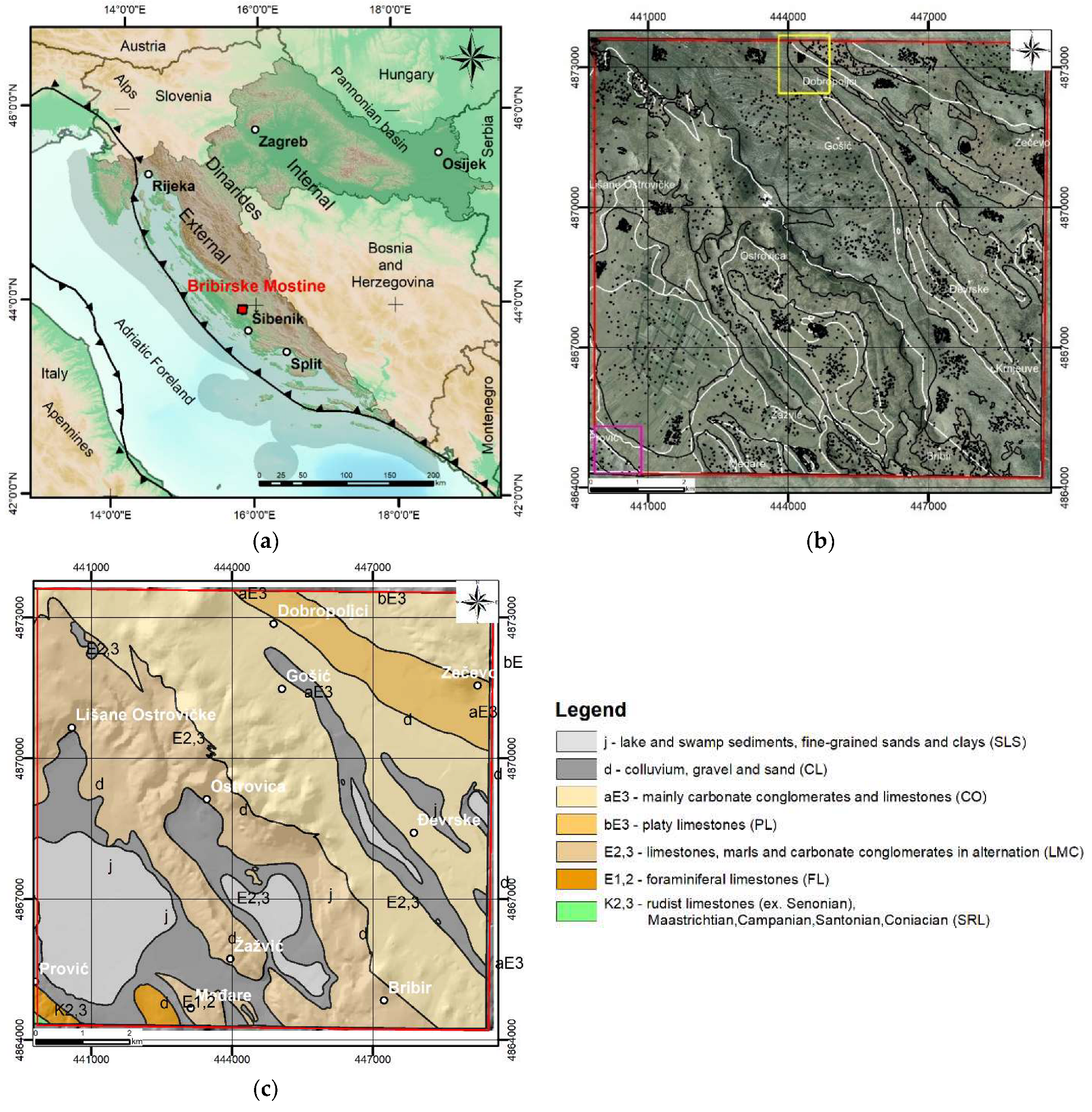
2.1. Study Area

The study area encompasses a part of the eastern Adriatic coastal region with an area of 8982 ha, situated in the central part of Northern Dalmatia, Croatia (Figure 1a). The relief includes the southern slopes of the Promina Mountains (Figure 1b). The study area is covered by the Basic Geological Map of the Yugoslavia (OGK SFRJ), sheet Šibenik, at a scale of 1:100,000 [26,27] and by the field geological map of the OGK SFRJ, sheet Bribirske Mostine, at a scale of 1:25,000 (Figure 1c). The terrain proved to be suitable due to the great exposure of outcrops, lack of vegetation and the geological potential of strategically important mineral resources for the Republic of Croatia. This area is part of the Croatian karst region of the Dinarides (Figure 1a), which is represented by a thick, largely carbonate succession deposited on carbonate platforms of different ages, types and paleogeographic settings from the Upper Carboniferous to the Eocene [18]. The oldest deposits on the Bribirske Mostine field geological map (Figure 1c) are rudist limestones (Figure 1c, Senonian, K_2,3), in which the percentage of CaCO₃ ranges from 95% to 99%. They range from microcrystalline to recrystallized limestones and, rarely, are dolomitized bioaccumulated limestones. Senonian rudist limestones (SRL) are used as dimension stone and/or as stone aggregates and are important mineral resources [28].

Paleogene deposits include Eocene foraminiferal limestones and calciclastic deposits of the Eocene and Lower Oligocene “Promina Beds” [27]. Eocene foraminiferal limestones (Figure 1c, E_1,2, FL) are well-layered, light-gray microcrystalline limestones containing up to 95–98% CaCO₃ and have significant potential for exploitation as dimension stone and/or stone aggregates [28]. The next three lithological units are part of the “Promina Beds”. The first is made up of fine-grained detrital to marly limestones with traces of marl and carbonate conglomerates (Figure 1c, E_2,3, LMC). Farther upward in the succession, two units consist of dominant carbonate conglomerates and alternations of these conglomerates with limestone and marls, as well as platy limestones (Figure 1c, aE₃ (CO), bE₃ (PL)). The lithological members of the “Promina Beds” can be exploited as raw materials in the cement industry as dimension stone and/or stone aggregates [28]. Quaternary sediments (Figure 1c,d (CL) and j (SLS)) consist mostly of gravel, sand and terra rosa. The colluvial (deluvial) deposits (Figure 1c,d, CL) are essentially deposits of weathered flysch, mostly gravels and sands of different grain sizes. These Quaternary sediments have geological potential for the exploitation of sand and gravel [28].

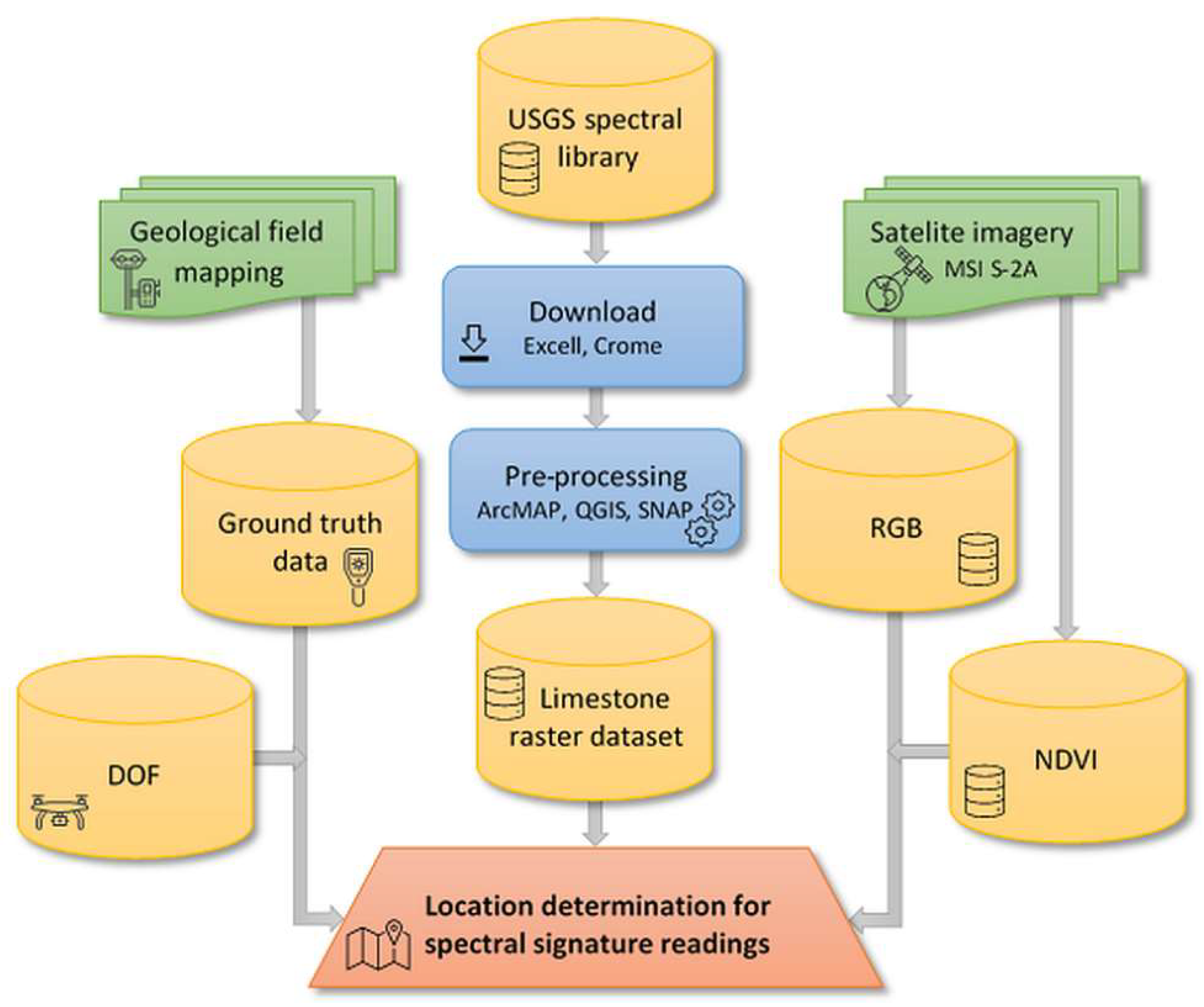
2.2. Datasets

The field geological map of the OGK SFRJ, sheet Bribirske Mostine, 1:25,000 (Figure 1c), a satellite image obtained with a multispectral sensor on Sentinel-2 satellites (MSI S-2A), the USGS spectral library data on limestones [30] and geological ground truth field data were used. Level-2A data using ortho-corrected bottom-of-atmosphere (BOA) data with subpixel multispectral notation were used [31]. During December 2021, two sites (Subsets 1 and 2) were geologically mapped. Subset 1 (Figure 2a) covers an area of 100 ha, where 36 observation points were recorded. Four (4) different lithological units were extracted: SRL, FL, CL and SLS (Figure 2a). The working principle was the same for Subset 2 (Figure 2b), covering an area of 134 ha. In this case, 35 geological field observation points were recorded, and two lithological units were singled out. These were PL and CO (Figure 2b).

2.3. Imagery Processing

At a medium scale, a digital form of the Bribirske Mostine geological map was created and transformed into the HTRS/96TM system. A zip file with title ID T33TWJ of 896,68 MB size was downloaded using the Copernicus Open Access Hub. The ingestion date was 2 April 2020. Resampling was used, the goal of which was to reduce the product to a single spatial resolution [15]. The resampling algorithm was bilinear, the downsampling method was mean and the flag downsampling method was first (Sentinel Applications Platform (SNAP) [32]). According to the SNAP transformations, the product was transformed from the WGS84 to the HTRS96/TM geographic system. First, the K-means algorithm was used [33,34]. Within the K-means classification, all bands of MSI S-2A were used, and a composite of bands 2, 3, 4, 8 and 11, all for 5, 10, 15 and 20 classes, was used separately.

The K-means algorithm is one of the simplest and most popular unsupervised classification algorithms, the aim of which is to divide M points in N dimensions into K clusters so that the within-cluster sum of squares is minimized. A matrix of M points in N dimensions and a matrix of K initial clusters are required as algorithm input data. Sets of objects are grouped in such a way that the objects in the same cluster (group) are as similar as possible. Similarity is determined by the distance between two data points, and the Euclidean distance is used to measure this distance [35,36]. The K-means algorithm objective is reducing the intra-cluster distance and increasing the distance between clusters [33,34,37,38]. This algorithm is currently used in numerous remote sensing projects [39,40,41]. For instance, a novel method based on a combination of spectral indices and K-means was developed for automatic land cover classification (ALCG, [42]).

The RF algorithm was subsequently used [43] to carry out the following important functions. The first was to serve as a means to conduct an impartial revision of the initial geological datasets, while the second was to serve as a basis for creating the final geological map [44,45]. In supervised classification, the user determines the input data, in this case, pixel values. After that, the algorithm uses the spectral signatures of the training sites and applies them to the entire image. It is a regression algorithm that works by creating a forest with decision trees, the object of which is to create a prediction model, the results of which are derived from a combination of different input variables. At the same time, the larger the number of trees in the forest, the more accurate the results [15,16,43,46,47]. The result of such a process, in this case, was a classified lithological map with unique and separable spectral signatures of each class. A review of machine learning in processing remote sensing data for mineral exploration was given by [48].

In this study, the input data for the RF classification were a K-means and DOF-derived geological map of Bribirske Mostine. Based on this map, 5200 circle polygons were selected to serve as ground truth data in RF classification. These polygons were placed on all lithological members, as shown in

Table 1. RF input polygon data for each lithological member.

No.	Label	Name	Area in km2	Surface Percentage %	No. of Polygons	Polygon Shape	Polygon Diameter (m)
1	j SLS	Lake and swamp sediments, fine-grained sands and clays	14.26	15.25	793	Circle	20
2	d CL	Colluvium, gravel and sand	27.24	29.17	1516	Circle	20
			26.63	28.51	1406
3	aE3 CO	Mainly carbonate conglomerates and limestones	20.94	22.42	1.166	Circle	20
4	bE3 PL	Platy limestones	12.91	13.82	719	Circle	20
			13.52	14.47	819
5	E2,3 LMC	Limestones, marls and conglomerates in alternation	16.37	17.53	911	Circle	20
6	E1,2 FL	Foraminiferal limestones	1.24	1.33	69	Circle	20
7	K2,3 SRL	Rudist limestones	0.25	0.27	14	Circle	20
8	a	Anomalies	0.20	0.22	12	Circle	20
9		Total area	93.39
10		Total percentage		100
11		Total polygons			5200

. It can be seen that a variant analysis was made for colluvium and platy limestones. The exact position of the input circle polygons is shown in Figure 1b.

The total number of circle polygons was determined in accordance with the surface distribution of each individual lithological member. The shape of the polygon was defined as a circle with a 10 m radius (20 m diameter). Such a radius was chosen due to the spatial resolution of MSI S-2A of 10 m. Due to possible deviations in the geometry of boundaries, the polygons were arranged in such a way that they were not positioned directly on the geological boundary. In the RF classification, the MSI S-2A band combination was used as in the K-means classification. Two variants of RF classification were considered. An account of the two variants of the RF classification is illustrated in the Results chapter. It is clearly marked with a red hachure.

Regarding large-scale maps (Figure 3), data collected from geological field mapping were used as ground truth data, i.e., validation data for Subset 1 and Subset 2 sites. The distribution of limestones in the study area was obtained by processing the USGS spectral library dataset. The NDVI was used to discriminate vegetation from the other forms of land cover [49]) and as a backup tool for evaluating the position of points or pixels (pins) on which spectral records were determined and statistically analyzed.

File T33TWJ was imported into SNAP. Selection points (Figure 4 and Figure 5) based on NDVI (Figure 4a and Figure 5a), the RGB composite (Figure 4b and Figure 5b), USGS limestone index (Figure 4c and Figure 5c), DOF (Figure 4a and Figure 5a), and ground truth data generated in ArcMap followed (Figure 2 and Figure 3). The main aim of using a combination of these five types of backgrounds was the maximum reduction of vegetation influence on spectral signature readings. Based on the location of these points (pins), 40 spectral signatures of each lithological unit were read and statistically processed. Six lithological unit spectral signatures were singled out (Figure 3 and Figure 6).

2.4. Discriminant Function Analysis

After spectral analysis (Figure 4, Figure 5, Figure 6 and Figure 7), a DFA was conducted on large-scale maps to obtain more precise data on the differences in spectral signatures within lithological units. In this study, DFA was used to explore the differences in the spectral index data-bearing potential for improving classifications in a few distinct lithologies mapped in the karst area of the Dinarides. In methodological terms, DFA is all about finding differences between a number of originally observed (natural) groups with the least possible margin of error made during classification [20,50,51]. In geology, it is regularly used in geochemistry, environmental geology or bauxite studies [52,53]. In this study, the purpose was to construct a predictive discriminant function model (DFM) with the highest possible classification efficacy, taking into account six a priori outlined groups of mapped lithological units (see legend in Figure 2)—CO, PL, SRL, FL, CL and SLS—and 12 variables representing the spectral indices derived from satellite band imagery—B1, B2, B3, B4, B5, B6, B7, B8, B8A, B9, B11 and B12.

3. Results

Based on the K-means algorithm maps (Figure 8) and DOF (Figure 1b), a satellite geological map of the Bribirske Mostine area was derived (Figure 9). The GBs derived in this way were compared with the original GBs of the Bribirske Mostine area (Figure 1b). The first result of the comparison was that the clearly observed difference in the geometry of GBs was not linear (Figure 1b). The second result concerned differences in the interpretation of lithological units, which were sorted into four (4) levels of differences (LODs, Figure 9 and Figure 10). Additionally, in Figure 9a, the lithological unit marked “CL, colluvium, gravel and sand” is highlighted with hachures in red. It was clearly extracted using the K-means algorithm (Figure 8) but was not in the original geological map (Figure 1c). Subset 2 site was geologically mapped during December 2021 (Figure 2b and Figure 9b,c). Then, it was concluded that this is an area represented by a lithological unit marked “bE₃, platy limestones, PL”, which follows the original geological map (Figure 1c). However, this area is covered with shallow soil with platy limestone (PL) fragments, as clearly shown in Figure 9d. By processing analog and K-means data results that correspond to ground truth data, apropos PL and CL exchanges were obtained, as shown in Figure 9d.

The results of digital satellite image processing using the RF algorithm (Figure 11) were presented as the relative difference between the original map and, thus, created geological maps. In all four cases (Figure 11a–d), the anomalies were clearly separable, in a very similar way to the K-means algorithm (Figure 8). In all four cases (Figure 11a–d), the lithological unit labeled “K_2,3, rudist limestones (ex. Senonian, Maastrichtian, Campanian, Santonian, and Coniacian) SRL”, was not extracted, nor was the GB between it and the lithological unit marked “E_1,2, foraminiferal limestones, FL”. In the first three cases (Figure 11a–c), in the southern part of the map, green-colored pixels were dissociated, which may indicate rudist limestones, while, in the fourth case, they were not. Based on ground truth data derived by geological field mapping, it was concluded that these were also anomalies caused by dense vegetation reflectance.

In the DFA of the investigated lithological units, six groups (K = 6) and twelve variables (descriptors, p = 12) were processed, resulting in a DFM of five discriminant functions (K − 1). Relevant multivariate tests were used before the analysis (

Table 2. Multivariate test regarding general significance of discrimination including tests of residual roots (DFs).

No. of variables				12
Wilks’ lambda				0.0024
Approximate F-ratio				45.979
Degrees of freedom				[60; 1048]
p-level				p = 0.000
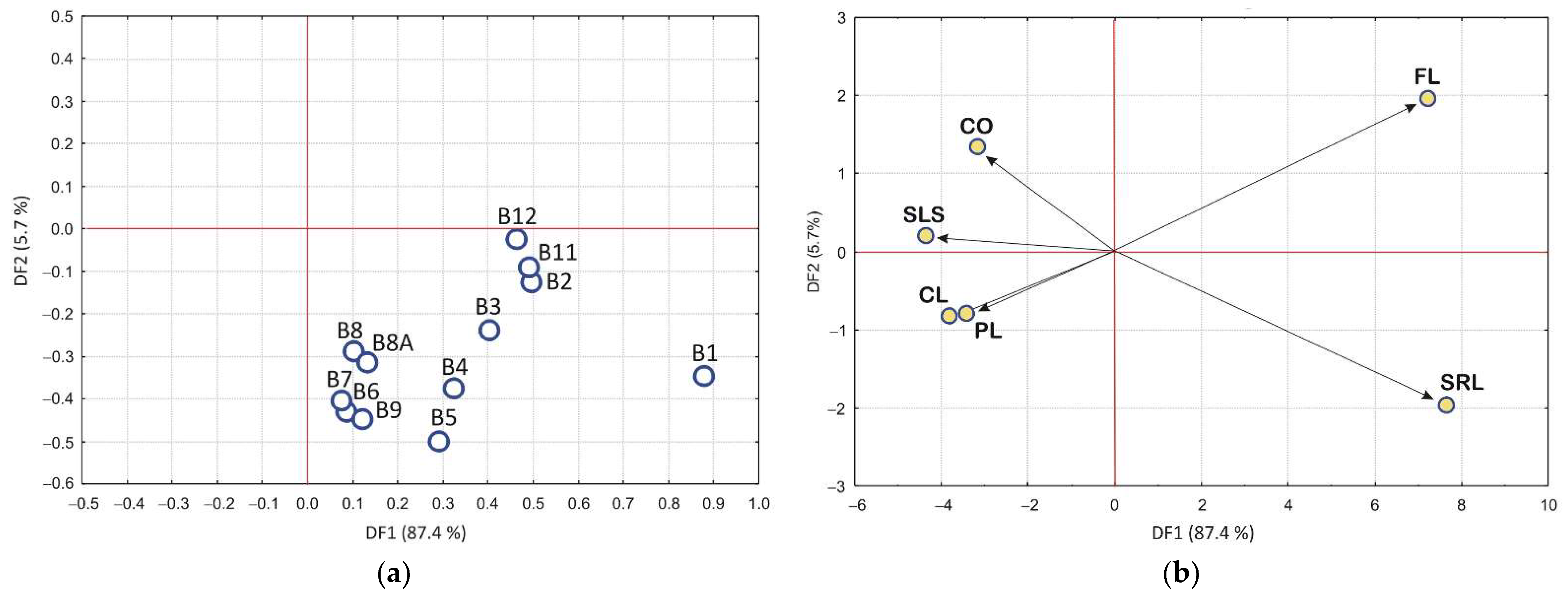
DF	Eigen value	Eigen (%)	Eigen cum.	Canon. R	Wilks’ λ	Chi2	df	p-Level
1	28.374	87.36	87.36	0.983	0.002	1389.2	60	0.000
2	1.854	5.71	93.07	0.806	0.070	611.8	44	0.000
3	1.101	3.39	96.46	0.724	0.200	370.6	30	0.000
4	0.885	2.72	99.18	0.685	0.419	199.8	18	0.000
5	0.265	0.82	100.00	0.458	0.791	54.0	8	0.000

), revealing extremely low associated probability (p = 0.000), a necessary precondition for the computation of discriminant functions (DFs). This breakdown process also included the univariate statistics of input data displayed as grouped boxplots for each band and lithological group (

Table 3. Breakdown table of descriptive statistics for each band and lithological group.

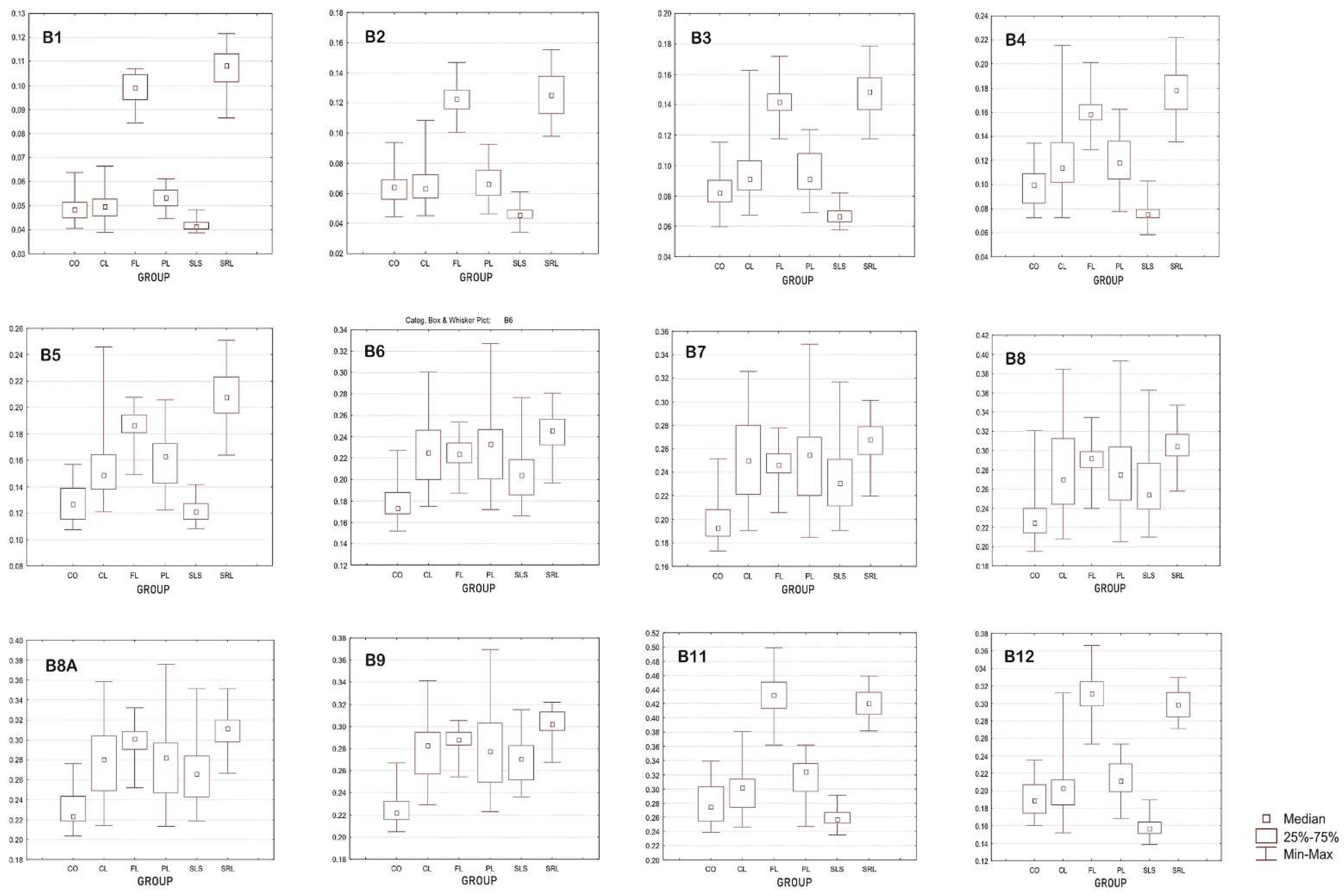
Group	Band	N	Mean	St. Dev.	Min	Max	Q1	Median	Q3
CO		40	0.049	0.005	0.041	0.064	0.045	0.048	0.052
CL		40	0.050	0.005	0.039	0.066	0.046	0.050	0.053
FL		40	0.098	0.006	0.085	0.107	0.094	0.099	0.105
PL	B1	40	0.053	0.005	0.045	0.061	0.050	0.053	0.057
SLS		40	0.042	0.002	0.039	0.048	0.040	0.041	0.043
SRL		40	0.107	0.009	0.086	0.122	0.102	0.108	0.113
All Groups		240	0.066	0.027	0.039	0.122	0.046	0.053	0.097
CO		40	0.063	0.010	0.044	0.094	0.056	0.064	0.069
CL		40	0.067	0.015	0.045	0.108	0.057	0.063	0.072
FL		40	0.122	0.010	0.100	0.147	0.116	0.123	0.129
PL	B2	40	0.067	0.011	0.047	0.092	0.058	0.066	0.075
SLS		40	0.047	0.006	0.034	0.061	0.043	0.046	0.049
SRL		40	0.126	0.015	0.098	0.155	0.113	0.125	0.138
All Groups		240	0.082	0.033	0.034	0.155	0.056	0.068	0.115
CO		40	0.084	0.012	0.060	0.115	0.076	0.082	0.090
CL		40	0.096	0.019	0.067	0.163	0.084	0.091	0.103
FL		40	0.142	0.011	0.117	0.172	0.136	0.142	0.147
PL	B3	40	0.095	0.015	0.069	0.124	0.084	0.091	0.108
SLS		40	0.068	0.006	0.058	0.082	0.063	0.066	0.070
SRL		40	0.149	0.015	0.118	0.179	0.137	0.148	0.158
All Groups		240	0.106	0.033	0.058	0.179	0.078	0.095	0.137
CO		40	0.098	0.016	0.072	0.134	0.084	0.100	0.109
CL		40	0.121	0.029	0.073	0.215	0.102	0.114	0.135
FL		40	0.159	0.012	0.129	0.201	0.153	0.158	0.166
PL	B4	40	0.120	0.020	0.078	0.162	0.104	0.118	0.136
SLS		40	0.077	0.009	0.058	0.103	0.072	0.075	0.079
SRL		40	0.178	0.019	0.135	0.222	0.163	0.178	0.191
All Groups		240	0.125	0.039	0.058	0.222	0.093	0.118	0.158
CO		40	0.128	0.013	0.108	0.157	0.115	0.127	0.139
CL		40	0.155	0.026	0.121	0.246	0.138	0.149	0.164
FL		40	0.186	0.013	0.149	0.208	0.181	0.187	0.194
PL	B5	40	0.161	0.022	0.122	0.206	0.143	0.163	0.173
SLS		40	0.122	0.008	0.108	0.142	0.116	0.121	0.127
SRL		40	0.212	0.019	0.164	0.251	0.196	0.208	0.223
All Groups		240	0.160	0.036	0.108	0.251	0.129	0.157	0.190
CO		40	0.178	0.016	0.152	0.227	0.168	0.173	0.188
CL		40	0.225	0.032	0.175	0.300	0.200	0.225	0.246
FL		40	0.223	0.015	0.187	0.254	0.216	0.224	0.234
PL	B6	40	0.230	0.036	0.172	0.327	0.201	0.233	0.247
SLS		40	0.206	0.026	0.166	0.276	0.185	0.204	0.219
SRL		40	0.245	0.017	0.196	0.281	0.232	0.246	0.257
All Groups		240	0.218	0.033	0.151	0.327	0.190	0.220	0.241
CO		40	0.198	0.017	0.173	0.252	0.186	0.192	0.208
DE		40	0.250	0.036	0.190	0.326	0.222	0.250	0.280
FL		40	0.246	0.016	0.206	0.278	0.239	0.247	0.256
PL	B7	40	0.252	0.037	0.185	0.349	0.220	0.255	0.270
SLS		40	0.234	0.029	0.190	0.317	0.211	0.231	0.251
SRL		40	0.268	0.017	0.219	0.301	0.255	0.268	0.279
All Groups		240	0.241	0.034	0.173	0.349	0.212	0.245	0.263
CO		40	0.229	0.023	0.195	0.321	0.214	0.225	0.240
CL		40	0.276	0.043	0.208	0.385	0.244	0.270	0.313
FL		40	0.290	0.018	0.240	0.334	0.282	0.292	0.299
PL	B8	40	0.279	0.044	0.205	0.393	0.249	0.275	0.304
SLS		40	0.262	0.034	0.210	0.363	0.239	0.254	0.287
SRL		40	0.305	0.017	0.258	0.347	0.294	0.304	0.317
All Groups		240	0.273	0.039	0.195	0.347	0.294	0.304	0.317
CO		40	0.230	0.018	0.204	0.276	0.219	0.223	0.243
CL		40	0.277	0.037	0.214	0.358	0.249	0.280	0.304
FL		40	0.298	0.018	0.252	0.332	0.290	0.301	0.308
PL	B8A	40	0.279	0.037	0.213	0.376	0.247	0.282	0.297
SLS		40	0.267	0.029	0.219	0.351	0.243	0.266	0.284
SRL		40	0.311	0.017	0.266	0.351	0.298	0.311	0.320
All Groups		240	0.277	0.037	0.204	0.376	0.244	0.282	0.305
CO		40	0.224	0.013	0.205	0.267	0.216	0.222	0.233
CL		40	0.279	0.031	0.229	0.341	0.257	0.283	0.295
FL		40	0.286	0.012	0.254	0.305	0.283	0.288	0.294
PL	B9	40	0.280	0.034	0.223	0.369	0.250	0.278	0.303
SLS		40	0.269	0.021	0.236	0.315	0.252	0.271	0.282
SRL		40	0.303	0.013	0.268	0.322	0.296	0.302	0.313
All Groups		240	0.274	0.033	0.205	0.369	0.245	0.282	0.296
CO		40	0.278	0.026	0.239	0.339	0.254	0.274	0.303
CL		40	0.299	0.032	0.247	0.381	0.274	0.302	0.314
FL		40	0.431	0.028	0.362	0.499	0.414	0.432	0.450
PL	B11	40	0.315	0.028	0.247	0.362	0.297	0.324	0.336
SLS		40	0.258	0.013	0.235	0.291	0.252	0.257	0.267
SRL		40	0.421	0.020	0.382	0.459	0.406	0.421	0.436
All Groups		240	0.334	0.072	0.235	0.499	0.270	0.313	0.407
CO		40	0.191	0.020	0.160	0.235	0.175	0.189	0.207
CL		40	0.205	0.034	0.152	0.312	0.184	0.203	0.212
FL	B12	40	0.312	0.022	0.253	0.366	0.297	0.311	0.325
PL		40	0.213	0.023	0.168	0.253	0.199	0.211	0.231
SLS		40	0.158	0.013	0.138	0.189	0.151	0.157	0.164
SRL		40	0.299	0.017	0.271	0.330	0.285	0.299	0.313
All Groups		240	0.230	0.061	0.138	0.366	0.178	0.211	0.293

Note: St. Dev. = standard deviation; Min = minimum; Max = maximum; Q1 = lower quartile; Q3 = upper quartile; and Med = median.

and Figure 12). Results showed (p-level and eigenvalue, Table 2) that the first two DFs, explaining over 93% of the total variance, effectively configure the discriminant space (Figure 13a,b).

Essential in DFA, is derivation of the functional model (describing natural, geological processes) out of the structural model (mathematical structure) of the analyzed data. To this effect, discriminant loadings are especially helpful in validating how much of the overall discrimination is explained by each separate variable (band). Reading DFA in functional terms highlights the natural (geological) processes which are assumed accountable for the pattern of the structural model derived from spectral index data. Clearly, in building the best discrimination strategy, all variables with small discriminant loadings can be safely discarded for interpretation.

In this regard, comparison between the variable and group diagrams (Figure 13a,b) was the most helpful technique for structure-to-function relation and elucidation of the key reasons for group separation. In the process, affiliation between variables and associated groups was always interpreted considering their joint position along the corresponding discriminant axis in both diagrams (Figure 13a,b).

Regularly, the mutual relationship between the variables and group means (centroids) along the respective DF defines the geological (via remote sensing technology) nature of a computed mathematical model.

By virtue of variables (multispectral imagery bands) assuming the role of process descriptors, each DF was labeled geologically, contributing to the overall separation of groups (lithological units). Thus, the first discriminant function (DF1) was indubitably the greatest discriminator, clarifying more than 87% of the total variation in the analyzed model and, together with DF2, just over 93%. Despite their high statistical significance (p = 0.000), other functions could be safely excluded from further analysis owing to their low contribution to discrimination between groups (low eigenvalues) and low capability of inferring the relevant geological process.

The scatterplots of variable loadings and group means (centroids, Figure 13b) were bipolar, separating the FL/SRL from both the CL/PL and CO/SLS groups. However, a closer inspection revealed that all descriptor variables (bands) loaded on the positive side of DF1, a peculiar situation suggesting that the discrimination between FL/SRL and other groups posted on the negative pole of DF1 on their respective diagram was based solely on the “inverse image”, that is, the “absence” of relevant descriptor variables. In practical terms, this means that the respective group pairs (CL/PL and CO/SLS) were characterized entirely by decreased values in all descriptor variables regarding FL/SRL. Additionally, B1 was the variable with the highest discriminant potential, while the rest was crammed in several clusters, possibly indicating a more parsimonious scheme of band selection in further investigations. These include B2/B11/B12, then B8/B8A and, finally, B6/B7/B9 as obvious variable clusters. The B3, B4 and B5 bands can be seen as “transitory” variables communicating between the aforementioned clusters (Figure 13). Eventually, owing to its highlighted position in the discriminant model, DF1 clearly underscored the central theme of the analysis—separation of distinct lithological units mapped in the karst area of the Dinarides based on selected spectral indices (bands) derived from satellite imagery.

This was established by the high discrimination of both limestone formations (SRL and FL) compared to other lithological units marked by increased values of all spectral indices (bands), particularly of B1 (followed by B2, B11 and B12). Further insight into spectral differentiation of the investigated lithological groups was not impeded by the inferior discriminant potential of DF2 (Figure 13). Allocating the abovementioned “inverse image” properties (the fourth quadrant variable clustering) to DF2, the latter was predominantly involved with isolating SRL from the FL group (Figure 13b). As with DF1, separation revolved around the “absence/presence” polarized rapport contrasting SRL with FL via the generally higher spectral indices of the former, particularly B5 but also B6/B7/B9, B4 and B1 and others most distant from the axis intersection, as seen from the scatterplot of variable loadings (Figure 13a) depicting the group distances.

4. Discussion

Existing geological maps are the basic input data for the creation of the mineral resources potentiality maps, which are, in turn, used in the construction of spatial plans as basic documents for the physical planning of a certain administrative areas (state, region, county). In addition to geological data, an integral part of spatial plans is the data of other territory users. In most cases, they are regularly updated and roughly correspond to the time frame of the spatial plan construction. However, updating the geological data of a wider area is demanding and requires a significant expenditure of time and financial resources.

Therefore, the possibility of finding an efficient way of updating existing geological maps was considered, with the aim of obtaining more precise data on the geology of the area. Further in the discussion, the facts about the existing geological maps that are used as input data are commented on, followed by a discussion in two parts. The first part refers to the applicability of ML algorithms for the correction of geological boundaries as the basic elements of a geological map, in this case, at the scale 1:25,000. The second part refers to the use of spectral signatures of rocks and statistics in extracting lithological members on detailed maps at the scale 1:10,000. It is discussed whether such methods can be used in more precise determination of mineral resources potential. The karst area of the Dinarides was chosen due to the availability of rock outcrops and lack of vegetation but also the presence of mineral resources that are strategically important for the Republic of Croatia.

The creation of the OGK SFRJ in the 1960s and 1970s provided a basic geological map which is the necessary basis for further geological research and planning, including research of mineral resources [54]. This map is based on a chronostratigraphic division, and, despite certain disadvantages in correlation with maps of neighboring countries or some neighboring sheets, it is still extensively used in research related to mineral resources. Its use in combination with digital GIS technology and numerous new, precisely obtained field data (GNSS, real-time kinematic (RTK), etc.) has revealed certain deviations from the recorded field data. These deviations are primarily related to the geometry of the GB. As mentioned before, there has been a lack of previous research on lithological unit discrimination within karst terrains using remote sensing methods. Therefore, there was an initiative by the authors to initiate these studies. Conversely, technology development, and, more recently, the development of machine learning algorithms, mathematics and statistics in general, has intensified on a global scale. However, due to a lack of previous research on the mapping of karst terrains, here, we initially explored basic K-means and RF tools. Following these results, efforts will certainly be made to further implement other remote sensing methods and their mutual combination.

By combining the results collected with the K-means algorithm and DOF, four (4) LODs were identified. It is important to emphasize that these were determined LODs in geological maps without further quantification. Ideally, because of the number of LODs, it would be best to conduct the remapping of the entire area. However, this is unlikely to occur in the foreseeable future, and, according to the data offered by modern methods of remote sensing, it is considered unnecessary. By qualitatively “reprocessing” the existing maps, it is possible to obtain very accurate data. In [45], it was concluded that K-means could be used in mapping lithology and affirmed that this method can be implemented in existing map enhancement. The results of the RF classification showed that, in all cases, the anomalies were dissociated in a similar way. It is very likely that this was applied to surface objects with more significant differences in composition compared to rocks or vegetation. The next result was that the lithological unit marked as “K_2,3, rudist limestones, SRL” was also not dissociated, nor was its GB with the lithological unit marked “E_1,2 foraminiferal limestones, FL”. Although they were formed under different temporal and spatial conditions, due to the very similar percentage of CaCO₃, they are very difficult to dissociate. In the fourth case (Figure 11d), RF did not dissociate green pixels, as it did in the first three cases shown in Figure 11a–c. In this case, the map shown in Figure 11d displays data very similar to the actual field situation compared with the previous three listed. Regarding RF, Figure 11d is considered the most representative for the area in terms of further exploration of mineral resources. If alternatives with colluvium were excluded, other geological relations were very satisfactory in this research stage. They could be used as a basis for the potential investigation of mineral resources. The effectiveness of ML techniques for classifying geological units based on multispectral maps was written about in [55]. With ML processing methods, existing geological boundaries can be corrected as basic elements of geological maps, which means that, in this way, geological maps can also be completed and can be used in delineating areas favorable for mineral exploration and exploitation through the creation of adequate mineral resources maps with accuracy that can be used in regional spatial plans at a scale of 1:25,000.

The raster-derived data based on the USGS limestone index agreed well with the field data. The reason is very likely due to the high content of CaCO₃ in rudist (SRL), foraminiferal (FL) and platy limestone (PL). In this case, the NDVI was used as an additional tool for the general separation of vegetation from other land cover types (mostly rocks). Being obtained by a reliable sensor, it was considered useful for this type of use [56]. In DFA, the classification efficiency has often demonstrated higher efficiency in discrimination than various statistical tests [20]. In this regard, classification rates of previously outlined lithostratigraphic units can be straightforwardly examined, comparing the mathematically “predicted” (calculated) and original (“natural”) group membership of single cases.

Table 4. Classification matrix of six lithological units (CO, CL, FL, PL, SLS, SRL).

Groups	CO	CL	FL	PL	SLS	SRL	% Correct
CO	38	0	0	2	0	0	95.00
CL	1	22	0	11	6	0	55.00
FL	0	0	36	0	0	4	90.00
PL	6	5	0	29	0	0	72.50
SLS	3	0	0	0	37	0	92.50
SRL	0	0	2	0	0	38	95.00
Total	48	27	38	42	43	42	83.33

Observed classifications (rows)—samples passed on other groups; Predicted classifications (columns)—samples obtained from other groups; a priori defined groups have an equal number of 40 samples each.

reveals that the DFM was structured with very high efficacy exceeding 80%. However, for some groups, such as CL and PL, overlapping was considerable, which was also evident from their low squared Mahalanobis distance (3.33,

Table 5. Squared Mahalanobis distances (SMD) between the investigated lithological groups (CO–SRL).

	CO	CL	FL	PL	SLS	SRL
CO	0.00	12.07	116.27	12.57	12.49	129.37
CL	12.07	0.00	130.90	3.33	9.57	136.98
FL	116.27	130.90	0.00	122.04	142.82	19.25
PL	12.57	3.33	122.04	0.00	11.08	128.68
SLS	12.49	9.57	142.82	11.08	0.00	152.59
SRL	129.36	136.98	19.25	128.68	152.60	0.00

) and, visually, from the respective group centroid diagrams (Figure 13b). In the abovementioned case, barely 22 of the 40 CL members were allocated to that specific group, whereas the remainder was lost to PL (11), SLS (6) and CL groups, collapsing the classification rate to a modest 55%. Given the PL group, the classification accuracy was slightly better and amounted to 72.5%. Here, 11 cases among the 40 were lost to other groups, including CO (6) and CL (5). This information indicates significant inhomogeneity of the CL lithological unit, the 45% allocations of which were unequivocally misclassified, showing remarkable cross-exchange with the PL group in particular (Table 4). Other groups were characterized by high classification rates, especially CO and SRL (95%).

In this paper, the authors tried to single out not only the types of limestone (Senonian rudist limestones (SRL) and Eocene foraminiferal limestones (FL), first type of discrimination) but also the sediments that are result of their weathering. The second type of discrimination refers to the “Promina Beds” sediments, which are known in the literature on karst terrains [19,57,58,59,60]. In this research, these sediments were represented by platy limestones (PL) and mainly carbonate conglomerates and limestones (CO). They were transported by strong currents which flowed from the raised Dinarides during the Eocene and Oligocene, eroded the carbonate platform sediments and deposited the weathered material in the land or marine sediment basins. The literature on the “Promina Beds” states that these sediments formed due to rapid changes in the river morphology, sudden fluctuations in flow and lack of stable banks. They also formed in marine conditions. This makes the lithological units PL and CO very similar, and it is often difficult to distinguish them in the field, as such sedimentary environments are extremely complex. The third type of lithological unit that has been singled out is Quaternary sediments (colluvium, gravel and sand (CL) and lake and swamp sediments, fine-grained sands and clays, SLS). They are also the weathering products of all previous lithological units and are usually additionally covered with a thin layer of soil. Therefore, they are also difficult to single out.

Using USGS spectral signatures and NDVI, the areas from which spectral signatures could be read were first selected, and these signatures were statistically processed. The obtained data indicated the possibility of distinguishing lithological members even within the complex karst terrain. This method is applicable in two ways. The first one refers to the validation of maps to the scale 1:25,000, while the second one refers to detailed geological mapping to the scale 1:10,000. This makes it possible to extract the potential of mineral resources in even more detail. DFA as a statistical method was also used as an additional tool for the validation of results, but also for proving the possibility of detailed separation of lithological members based on spectral signatures.

5. Conclusions

This paper emphasized that the rapid development of digital technologies enables research of mineral resources in karst terrains. Using the K-means algorithm, a lithological unit that was not dissociated in the original geological map was displayed at an early stage of the research. Its dissociation is important because its subsequently calculated quantities can significantly affect the geological potential of the study area. The K-means algorithm additionally showed its importance in outlier extraction. By processing the Sentinel-2A data, different lithological units with a carbonate composition were also extracted, but not without field validation and/or in combination with one of the supervised classification methods. In this case, the existing geological maps were finely, digitally processed, and the K-means algorithm with the DOF and field validation enabled their geometric correction. The GBs derived by ML algorithms were more precisely determined than before and can be used with greater precision when calculating geological potential. The supervised classification using the RF algorithm showed great potential in exploring mineral resources because it successfully divided the research area into given classes, although it was found to be mainly carbonate terrain. The supervised classification on raster datasets using USGS indices met its expectations exclusively as a support instrument, not for the absolute separation of lithological units. The NDVI also proved its value as a support tool. Finally, DFA showed its immeasurable potential in separating lithological units scanned by remote sensing and treated in the form of multispectral satellite data.

The use of ML algorithms made it possible to correct the geological boundaries by one order of magnitude, that is, the determined error in the geometry of the geological boundaries was reduced from the established 300 m to below 100 m. This is very significant for maps to the scale 1:25,000, since these data are directly used during spatial planning. In karst terrains without a significant percentage of vegetation, it is also possible to use spectral signatures. By integrating them into geological maps, the data can be displayed on an even more detailed scale, even to the scale of 1:10,000. This has not been the case so far. More precisely obtained geological data later result in more precise spatial plans, which is very important for other territory users but also for economic activities in a certain administrative unit. In addition to the above, the authors highlight the topic’s importance for the wider region, such as the Alpine–Dinaric karst area, Southeast Europe, etc.

References

- Gupta, R.P. Remote Sensing Geology, 3rd ed.; Springer: Berlin/Heidelberg, Germany, 2018; pp. 1–428. [Google Scholar] [CrossRef]
- Bishop, C.; Rivard, B.; de Souza Filho, C.; van der Meer, F. Geological Remote Sensing. Int. J. Appl. Earth Obs. Geoinf. 2018, 64, 267–274. [Google Scholar] [CrossRef]
- Oluić, M. Tektonska analiza graničnog područja Hrvatske i Slovenije izrađena na snimcima napravljenim iz satelita ERTS-1. Geol. Vje. 1975, 28, 87–96. [Google Scholar]
- Oluić, M. Neke karakteristike tektonike u graničnom području Crne Gore, Dalmacije i Hercegovine na osnovi Landsat snimaka. Geol. Vje. 1979, 24–25, 43–49. [Google Scholar]
- Oluić, M. Snimanje i Istraživanje Zemlje iz Svemira; Hrvatska akademija znanosti i umjetnosti: Zagreb, Republika Hrvatska, 2001; pp. 10–516. [Google Scholar]
- Tangestani, M.H.; Shayeganpour, S. Mapping a Lithologically Complex Terrain Using Sentinel-2A Data: A Case Study of Suriyan Area, Southwestern Iran. Taylor Fr. 2020, 41, 3558–3574. [Google Scholar] [CrossRef]
- Karimzadeh, S.; Tangestani, M.H. Potential of Sentinel-2 MSI Data in Targeting Rare Earth Element (Nd3+) Bearing Minerals in Esfordi Phosphate Deposit, Iran. Egypt. J. Remote Sens. Space Sci. 2022, 25, 697–710. [Google Scholar] [CrossRef]
- Ibrahim, E.; Barnabé, P.; Ramanaidou, E.; Pirard, E. Mapping Mineral Chemistry of a Lateritic Outcrop in New Caledonia through Generalized Regression Using Sentinel-2 and Field Reflectance Spectra. Int. J. Appl. Earth Obs. Geoinf. 2018, 73, 653–665. [Google Scholar] [CrossRef]
- Purwadi, I.; van der Werff, H.M.; Lievens, C. Targeting rare earth element bearing mine tailings on Bangka Island, Indonesia, with Sentinel-2 MSI. Int. J. Appl. Earth Obs. Geoinf. 2020, 88, 102055. [Google Scholar] [CrossRef]
- Shebl, A.; Abdellatif, M.; Hissen, M.; Abdelaziz, I.A.; Csámer, Á. Lithological mapping enhancement by integrating Sentinel 2 and gamma-ray data utilizing support vector machine: A case study from Egypt. Int. J. Appl. Earth Obs. Geoinf. 2021, 105, 102619. [Google Scholar] [CrossRef]
- Qi, X.; Zhang, C.; Wang, K. Comparing remote sensing methods for monitoring karst rocky desertification at sub-pixel scales in a highly heterogeneous karst region. Sci. Rep. 2019, 9, 13368. [Google Scholar] [CrossRef] [Green Version]
- Horvat, B.; Rubinić, J. Evaluating the Applicability of Thermal Infrared Remote Sensing in Estimating Water Potential of the Karst Aquifer: A Case Study in North Adriatic, Croatia. Remote Sens. 2021, 13, 3737. [Google Scholar] [CrossRef]
- Van der Meer, F.D.; van der Werff, H.M.A.; van Ruitenbeek, F.J.A. Potential of ESA’s Sentinel-2 for Geological Applications. Remote Sens. Environ. 2014, 148, 124–133. [Google Scholar] [CrossRef]
- Alpaydin, E. Introduction to Machine Learning, 4th ed.; The MIT Press: Cambridge, MA, USA; London, UK, 2020; p. 712. [Google Scholar]
- Cracknell, M.J. Machine Learning for Geological Mapping: Algorithms and Applications. Ph.D. Thesis, University of Tasmania, Hobart, Australia, 2014; pp. 1–275. [Google Scholar]
- Cracknell, M.J.; Reading, A.M. Geological Mapping Using Remote Sensing Data: A Comparison of Five Machine Learning Algorithms, Their Response to Variations in the Spatial Distribution of Training Data and the Use of Explicit Spatial Information. Comput. Geosci. 2014, 63, 22–33. [Google Scholar] [CrossRef] [Green Version]
- Cracknell, M.J.; Reading, A.M.; McNeill, A.W. Mapping Geology and Volcanic-Hosted Massive Sulfide Alteration in the Hellyer–Mt Charter Region, Tasmania, Using Random ForestsTM and Self-Organising Maps. Aust. J. Earth Sci. 2014, 61, 287–304. [Google Scholar] [CrossRef]
- Vlahović, I.; Tišljar, J.; Velić, I.; Matičec, D. Evolution of the Adriatic Carbonate Platform: Palaeogeography, Main Events and Depositional Dynamics. Palaeogeogr. Palaeoclimatol. Palaeoecol. 2005, 220, 333–360. [Google Scholar] [CrossRef]
- Zupanič, J.; Babić, L. Sedimentary Evolution of an Inner Foreland Basin Margin: Palaeogene Promina Beds of the Type Area, Mt. Promina (Dinarides, Croatia). Geol. Croat. 2011, 64, 101–119. [Google Scholar] [CrossRef]
- Rock, N.M.S. Numerical Geology. A source guide, glossary and selective bibliography to geological uses of computers and statistics. In Lecture Notes in Earth Sciences; Bhattacharji, S., Friedman, G.M., Neugebauer, H.J., Seilacher, A., Eds.; Springer: Berlin/Heidelberg, Germany, 1988; Volume 18, pp. 1–379. [Google Scholar]
- Rodriguez-Galiano, V.; Sanchez-Castillo, M.; Chica-Olmo, M.; Chica-Rivas, M. Machine Learning Predictive Models for Mineral Prospectivity: An Evaluation of Neural Networks, Random Forest, Regression Trees and Support Vector Machines. Ore Geol. Rev. 2015, 71, 804–818. [Google Scholar] [CrossRef]
- Lary, D.J.; Alavi, A.H.; Gandomi, A.H.; Walker, A.L. Machine Learning in Geosciences and Remote Sensing. Geosci. Front. 2016, 7, 3–10. [Google Scholar] [CrossRef] [Green Version]
- Othman, A.A.; Gloaguen, R. Integration of Spectral, Spatial and Morphometric Data into Lithological Mapping: A Comparison of Different Machine Learning Algorithms in the Kurdistan Region, NE Iraq. J. Asian Earth Sci. 2017, 146, 90–102. [Google Scholar] [CrossRef]
- Talukdar, S.; Singha, P.; Mahato, S.; Pal, S.; Liou, Y.A.; Rahman, A. Land-Use Land-Cover Classification by Machine Learning Classifiers for Satellite Observations-A Review. Remote Sens. 2020, 12, 1135. [Google Scholar] [CrossRef] [Green Version]
- Shirmard, H.; Farahbakhsh, E.; Heidari, E.; Pour, A.B.; Pradhan, B.; Müller, D.; Chandra, R. A Comparative Study of Convolutional Neural Networks and Conventional Machine Learning Models for Lithological Mapping Using Remote Sensing Data. Remote Sens. 2022, 14, 819. [Google Scholar] [CrossRef]
- Mamužić, P.; Korolija, B.; Majcen, Ž.; Borović, I.; Magaš, N.; Bojanić, L.; Božićević, S.; Babić, L.; Šimunić, A. Osnovna Geološka Karta SFRJ 1:100000, List Šibenik K 33-8. Inst. Geol. Istrž. Zagreb (1962-1965); Savezni geološki zavod: Beograd, Serbia, SFRJ, 1971. [Google Scholar]
- Mamužić, P.; Vrsalović, I.; Muldini-Mamužić, S.; Korolija, B.; Majcen, Ž.; Borović, I. Osnovna Geološka Karta SFRJ 1:100000: Tumač za List Šibenik K 33-8. Inst. Geol. Istrž. Zagreb (1966); Savezni geološki zavod: Beograd, Serbia, SFRJ, 1975. [Google Scholar]
- Marković, S. Hrvatske Mineralne Sirovine; Institut za geološka istraživanja: Zagreb, Croatia, 2002; pp. 1–544. [Google Scholar]
- Korbar, T. Orogenic Evolution of the External Dinarides in the NE Adriatic Region: A Model Constrained by Tectonostratigraphy of Upper Cretaceous to Paleogene Carbonates. Earth-Sci. Rev. 2009, 96, 296–312. [Google Scholar] [CrossRef]
- Kokaly, R.F.; Clark, R.N.; Swayze, G.A.; Livo, K.E.; Hoefen, T.M.; Pearson, N.C.; Wise, R.A.; Benzel, W.M.; Lowers, H.A.; Driscoll, R.L.; et al. USGS Spectral Library Version 7. U.S. Geol. Surv. Data Ser. 2017, 1035, 61. [Google Scholar] [CrossRef] [Green Version]
- Gascon, F.; Bouzinac, C.; Thépaut, O.; Jung, M.; Francesconi, B.; Louis, J.; Lonjou, V.; Lafrance, B.; Massera, S.; Gaudel-Vacaresse, A.; et al. Copernicus Sentinel-2A Calibration and Products Validation Status. Remote Sens. 2017, 9, 584. [Google Scholar] [CrossRef] [Green Version]
- Press, W.H.; Teukolsky, S.A.; Vetterling, W.T.; Flannery, B.P. Numerical Recipes in C: The Art of Scientific Computing, 2nd ed.; Cambridge University Press: New York, NY, USA, 1992; pp. 1–965. [Google Scholar]
- Hartigan, J.A. Clustering Algorithms; John Wiley & Sons: New York, NY, USA, 1975; pp. 1–347. [Google Scholar]
- Hartigan, J.A.; Wong, M.A. Algorithm AS 136: A k-means clustering algorithm. J. R. Stat. Soc. Ser. C-Appl. Stat. 1979, 28, 100–108. [Google Scholar] [CrossRef]
- Liberti, L.; Lavor, C. Euclidean Distance Geometry; Springe: Cham, Switzerland, 2017; 133p. [Google Scholar] [CrossRef]
- Maor, E. The Pythagorean Theorem: A 4000-Year History; Princeton University Press: Princeton, NJ, USA, 2019; 296p. [Google Scholar] [CrossRef]
- Jain, A.K. Data Clustering: 50 Years beyond K-Means. Pattern Recognit. Lett. 2010, 31, 651–666. [Google Scholar] [CrossRef]
- Richards, J.A. Remote Sensing Digital Image Analysis: An Introduction, 5th ed.; Springer: Berlin/Heidelberg, Germany, 2013; pp. 1–494. [Google Scholar] [CrossRef]
- Celik, T. Unsupervised Change Detection in Satellite Images Using Principal Component Analysis and κ-Means Clustering. IEEE Geosci. Remote Sens. Lett. 2009, 6, 772–776. [Google Scholar] [CrossRef]
- Vattani, A. K-Means Requires Exponentially Many Iterations Even in the Plane. In Proceedings of the twenty-fifth annual symposium on Computational geometry, Aarhus, Denmark, 8–10 June 2009; pp. 324–332. [Google Scholar] [CrossRef] [Green Version]
- Di Giuseppe, M.G.; Troiano, A.; Troise, C.; De Natale, G. K-Means Clustering as Tool for Multivariate Geophysical Data Analysis. An Application to Shallow Fault Zone Imaging. J. Appl. Geophys. 2014, 101, 108–115. [Google Scholar] [CrossRef]
- Gašparović, M.; Zrinjski, M.; Gudelj, M. Automatic Cost-Effective Method for Land Cover Classification (ALCC). Comput. Environ. Urban Syst. 2019, 76, 1–10. [Google Scholar] [CrossRef]
- Breiman, L. Random Forests. Mach. Learn. 2001, 45, 5–32. [Google Scholar] [CrossRef] [Green Version]
- Cracknell, M.J.; Reading, A.M. The Upside of Uncertainty: Identification of Lithology Contact Zones from Airborne Geophysics and Satellite Data Using Random Forests and Support Vector Machines. Geophysics 2013, 78, WB113–WB126. [Google Scholar] [CrossRef]
- Kuhn, S.; Cracknell, M.J.; Reading, A.M. Lithological Mapping in the Central African Copper Belt Using Random Forests and Clustering: Strategies for Optimised Results. Ore Geol. Rev. 2019, 112, 103015. [Google Scholar] [CrossRef]
- Harris, J.R.; Grunsky, E.C. Predictive Lithological Mapping of Canada’s North Using Random Forest Classification Applied to Geophysical and Geochemical Data. Comput. Geosci. 2015, 80, 9–25. [Google Scholar] [CrossRef]
- Darijani, M.; Farquharson, C.G.; Perrouty, S. A Random Forest approach to predict geology from geophysics in the Pontiac subprovince, Canada. Can. J. Earth Sci. 2022, 59, 489–503. [Google Scholar] [CrossRef]
- Shirmard, H.; Farahbakhsh, E.; Müller, R.D.; Chandra, R. A Review of Machine Learning in Processing Remote Sensing Data for Mineral Exploration. Remote Sens. Environ. 2022, 268, 112750. [Google Scholar] [CrossRef]
- Weier, J.; Herring, D. Measuring Vegetation (NDVI and EVI); NASA Earth Observatory: Washington, DC, USA, 2000. [Google Scholar]
- Davis, J.C. Statistics and Data Analysis in Geology, 2nd ed.; John Wiley & Sons: New York, NY, USA, 1986. [Google Scholar]
- Dillon, W.; Goldstein, M. Multivariate Analysis: Methods and Applications; John Wiley & Sons: New York, NY, USA, 1984. [Google Scholar] [CrossRef]
- Peh, Z.; Kovačević Galović, E. Geochemistry of Istrian Lower Palaeogene Bauxites—Is It Relevant to the Extent of Subaerial Exposure during Cretaceous Times? Ore Geol. Rev. 2014, 63, 296–306. [Google Scholar] [CrossRef]
- Hasan, O.; Miko, S.; Ilijanić, N.; Brunović, D.; Dedić, Ž.; Šparica Miko, M.; Peh, Z. Discrimination of Topsoil Environments in a Karst Landscape: An Outcome of a Geochemical Mapping Campaign. Geochem. Trans. 2020, 21, 1. [Google Scholar] [CrossRef] [PubMed]
- Plummer, C.; Carlson, D.; Hammersley, L. Physical Geology, 14th ed.; McGraw-Hill Education: New York, NY, USA, 2012. [Google Scholar]
- Kovačevič, M.; Bajat, B.; Trivič, B.; Pavlovič, R. Geological Units Classification of Multispectral Images by Using Support Vector Machines. In Proceedings of the International Conference on Intelligent Networking and Collaborative Systems, Barcelona, Spain, 4–6 November 2009; pp. 267–272. [Google Scholar] [CrossRef]
- Huang, S.; Tang, L.; Hupy, J.P.; Wang, Y.; Shao, G. A Commentary Review on the Use of Normalized Difference Vegetation Index (NDVI) in the Era of Popular Remote Sensing. J. For. Res. 2021, 32, 1–6. [Google Scholar] [CrossRef]
- Mrinjek, E. Conglomerate fabric and paleocurrent measurement in the braided fluvial system of the Promina Beds in northern Dalmatia (Croatia). Geol. Croat. 1993, 46, 125–136. [Google Scholar] [CrossRef]
- Mrinjek, E. Sedimentology and depositional setting of alluvial Promina Beds in northern Dalmatia, Croatia. Geol. Croat. 1993, 46, 243–261. [Google Scholar] [CrossRef]
- Babić, L.; Zupanić, J.; Kurtanjek, D. Sharply-topped alluvial gravel sheets in the Palaeogene Promina Basin (Dinarides, Croatia). Geol. Croat. 1995, 48, 33–48. [Google Scholar] [CrossRef]
- Babić, L.; Zupanič, J. Major events and stages in the sedimentary evolution of the Paleogene Promina basin (Dinarides, Croatia). Nat. Croat. Period. Musei Hist. Nat. Croat. 2007, 16, 215–232. [Google Scholar]