

A Continuous PDR and GNSS Fusing Algorithm for Smartphone Positioning
1
School of Transportation, Southeast University, Nanjing 210096, China
2
Airport Department, Civil Aviation Administration of China, Beijing 100028, China
3
School of Instrument Science and Engineering, Southeast University, Nanjing 210096, China
*
Author to whom correspondence should be addressed.
Remote Sens. 2022, 14(20), 5171; https://0-doi-org.brum.beds.ac.uk/10.3390/rs14205171
Submission received: 29 September 2022
/
Revised: 11 October 2022
/
Accepted: 11 October 2022
/
Published: 16 October 2022
(This article belongs to the Special Issue Integrated Applications of Real-Time GNSS Precise Positioning Services)
Abstract
:Pedestrian dead reckoning (PDR), used in state-of-the-art smartphones, calculates pedestrian positions by using built-in inertial sensors. However, the complex and changeable usage modes of smartphones have been obstructing the development of PDR in the field of gait detection. Since the measurement of the sensor is affected by noise, position errors will emerge, needing to be corrected periodically via external measurements. To this end, an optimization-based PDR (OBPDR) method for smartphones is proposed in this study. First, an improved finite state machine (IFSM) gait detection method is designed, which can improve the gait recognition rate and stability compared with the traditional peak detection method. Second, the step detection algorithm proposed in this paper is combined with a heading estimation to obtain the PDR dynamic model. Finally, the measurements of GNSS are fused to the PDR model, based on an adaptive extended Kalman filter (AEKF) algorithm, which can enhance the adaptability of the system to the environment in order to reduce the cumulative errors of PDR. Experiments are carried out to evaluate the performance of the proposed method. The results indicate that compared with the gait detection method, based on peak detection, and the integrated positioning method, based on an extended Kalman filter, the proposed method boasts favorable robustness and a high gait recognition rate, the recognition accuracy being kept between 97.5% and 98.5%; the average position error decreased by more than 67.25%.
1. Introduction
With the rapid development of 5G and the Internet of Things (IoT), location-based services (LBS) can be applied to an increasing variety of electronic devices, including smartphones, iPads, smart wearable devices, etc. [1,2,3]. LBS have facilitated public life with applications in various aspects, such as artificial intelligence (AI), the smart city, emergency rescue, traffic services, and public safety, becoming indispensable tools for people in modern society [4,5]. At present, positioning in smartphones is studied in conjunction with technologies such as Wi-Fi [6], GNSS [7], Bluetooth [8], gyroscopes, acceleration, magnetic sensors, light, pressure transducers, temperature sensors, etc. Hence, the research on location technology based on smartphones shows bright prospects and good feasibility.
Due to the advantages of smartphones with built-in micro electromechanical system sensors (MEMS), such as being lightweight and of small size, with low power consumption, low cost, easy integration, and so on, the pedestrian dead reckoning (PDR) method, based on MEMS sensors, has been widely studied by many scholars [9,10,11]. PDR consists of gait detection and step and heading estimation. Gait detection is used for identifying the movements of pedestrians and providing step frequency information for step size estimation, and can also synchronously control heading output and the fusion positioning trigger for multi-source fusion indoor positioning [12]. Therefore, gait detection is a core factor in PDR. Generally, the following methods are used for gait detection: peak detection, autocorrelation analysis, spectrum analysis, zero-crossing [13], and finite state machine (FSM) methods [14]. The principle of the peak detection method is to detect the number of peaks in an acceleration cycle. However, errors are often created when the number of peaks is recorded as the number of walking steps, thus weakening the credibility of step-counting results [15,16]. The autocorrelation analysis algorithm detects the step by analyzing the correlation between acceleration time series [17,18,19]. The spectral analysis method converts the time domain into the frequency domain to realize the step-counting function [20]. However, autocorrelation analysis and spectral analysis, which need a fixed and long-term window, have the disadvantages of large computational demand and high complexity [21]. The zero-crossing method is mostly used for foot-mounted inertial navigation because it needs to perceive the zero value of acceleration or angular velocity and is not applicable to smartphones. Alzantot studied the gait detection method based on the finite state machine (FSM) [22]. Four acceleration thresholds were set to judge the start, peak, trough, and end states; however, using only the acceleration threshold to identify gait offers poor universality. The FSM method proposed by Wang divides the gait cycle into three states to avoid the false threshold and the interference of false peaks [23]. However, only the static and moving states of pedestrians were studied, while other moving states were not considered. Xu proposed the gait detection of a finite state machine based on six states, wherein the state is converted through the set threshold. However, the detection performance of the algorithm has not been verified to be effective in other activities [24].
In this paper, an optimization-based PDR (OBPDR) method is proposed for smartphone positioning. The main contributions of our research are as follows: (1) a gait detection method based on an improved finite state machine (IFSM). In the IFSM method, the gait cycle of pedestrians is divided into five states, according to the characteristics of the acceleration waveform of “increase—peak—decrease—valley” during walking, which corresponds to the trend of resultant acceleration. More accurate step recognition is achieved by using the difference between adjacent resultant acceleration and the threshold of upslope and downslope times. (2) In order to obtain the PDR dynamic model, the step detection algorithm proposed in this paper is combined with a heading estimation. (3) To suppress the cumulative error of PDR, the measurements of GNSS are fused with the PDR measurements using an adaptive extended Kalman filter (AEKF), which enhances the adaptability of the system to the environment. By correcting the cumulative error of PDR results and the point-drift error of GNSS positioning, a high-precision PDR solution is obtained. The OBPDR method has been verified effectively by experiments in different environments.
The remainder of this paper is organized as follows. The model and characteristics of the traditional peak detection of PDR are briefly assessed in Section 2. In Section 3, the data preprocessing, the IFSM algorithm, the dynamic model of PDR, and the data fusion of GNSS and PDR, based on the AEKF algorithm, are introduced in detail. The experimental equipment and analyses of the results are introduced in Section 4. Finally, the conclusions drawn from this work are presented in Section 5.
2. PDR Model and Its Characteristics
2.1. Peak Detection
The basic principle of the peak detection method is to detect the acceleration value of each epoch, where each detected peak is recorded as a step. This method boasts a simple model, small computing resources, strong real-time performance, and easy implementation. However, it is necessary to identify a large number of pseudo peaks and the method requires high threshold accuracy. According to the periodic characteristics of changes where the acceleration will increase and decrease in every step of walking, it can be inferred that there must be a one-to-one correspondence between the true peak and the true valley in each gait of each traveler, so the peak and valley can be confirmed through time-series matching. The method can be divided into three steps.
Firstly, the peak and valley points are detected by Equation (1).
where and are the local peak and valley at the sampling points and ; and are the peak and valley thresholds, respectively; represents the value of acceleration, with subscript being , , , and , recording the number of peaks and valleys as and , respectively. The symbol represents “and”. When a peak point is detected, is increased by 1; similarity, when a valley point is detected, is increased by 1.
Secondly, we judge whether the first local extreme value that is detected is a local peak or a local valley, to ensure that the peak and valley points meet the constraints of a set of ordered pairs, as shown in Equation (2):
where denotes a marking point. If the first extreme point detected is a local peak, is recorded as 1. Otherwise, it is considered to be the local valley and is recorded as 0.
Lastly, the pseudo peak and pseudo valley at each sampling point need to be eliminated during the process of detecting local peaks and valleys.
If one part of Equation (3) is satisfied, there is a pseudo peak between the detected peak and the previous one. If , the peak point needs to be eliminated; otherwise, needs to be eliminated:
Similarly, when a local valley is detected, it is judged, according to Equation (4), that if either of them is satisfied, then this indicates that there is a pseudo valley at the sampling points and . If , the peak point needs to be eliminated; otherwise, needs to be eliminated:
Using the above constraints, not only can the peak and valley value points of time-sequence matching be obtained, but the pseudo peaks and pseudo valleys in the resultant acceleration signal can also be eliminated effectively. In this way, the accuracy of gait detection is improved.
2.2. Problem Formulation
At present, smartphones use built-in MEMS sensors, such as accelerometers, gyroscopes, magnetometers, and gravimeters to produce measurements for PDR indoor positioning [25,26]. The process of PDR positioning is shown in Figure 1, in which the PDR positioning based on a smartphone is divided into three steps: gait detection, step estimation, and heading estimation. The use of PDR for positioning excels in terms of independent positioning, due to its relatively low cost and operation, without additional equipment and base station deployment.
In the PDR algorithm, each dead reckoning is implemented at the end of each gait cycle. Generally, gait detection and step count are carried out using a pedometer or accelerometer. The heading angle is obtained by using a gyroscope or magnetometer. The PDR algorithm can provide location information for pedestrians in a two-dimensional plane. Its accuracy mainly depends on the accuracy of gait detection. The most common method of gait detection is peak detection. However, relying solely on a peak detection method will lead to invalid step counting because the non-walking action and handshake make it difficult to distinguish false peaks. Therefore, it is essential to improve the step accuracy while maintaining the low computational complexity of the traditional peak detection method.
The built-in MEMS sensors of smartphones are undesirable due to their high noise, low precision, and poor stability, and the positioning error increases over time. An error in heading, in particular, will double the positioning error. Therefore, it is necessary to reduce measurement errors in combination with other information. At present, GNSS plays an important role in users’ lives as it can provide global services with smartphones [27,28]. Good results can be attained with satellite navigation and positioning in open areas. However, being limited by the low-cost antenna of smartphones, large GNSS signal attenuation leads to a rapid decline in positioning performance in complex environments such as urban valleys. Hence, it is very important to effectively integrate MEMS sensors and GNSS positioning chips into smartphones to compensate for their respective defects and improve the positioning capability of the system.
3. The Proposed OBPDR Method
3.1. IFSM Gait Detection Algorithm
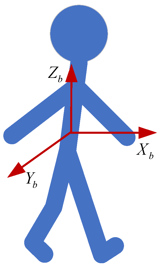
The acceleration, angular rate, and other information regarding pedestrians are collected with smartphones. In this study, the acceleration generated during walking is used to realize step-counting. Figure 2 shows the walking components of a pedestrian, with the origin at the pedestrian's center of gravity. The -axis, -axis, and -axis point to the forward, lateral and vertical, respectively.
The 3-axis acceleration time series of the pedestrian is shown in Figure 3. It can be observed from the enlarged sub-figure that the waveform of the collected three-axis acceleration is similar to a sine wave, with a certain periodicity.
The output frequency range of the built-in accelerometer of the smartphone is generally 15–200 Hz [29]. In this study, the output frequency of the mobile phone is set to 50 Hz.
The coordinate axis of the accelerometer deviates from the walking components of pedestrians, as shown in Figure 2, due to the various postures in which pedestrians hold their phones. In order to eliminate the influence of the directional changes of the smartphone, the resultant acceleration is used to calculate the acceleration norm, denoted as , by computing the Euclidean norm:
where , with , denotes the acceleration along the , , and axes, respectively.
Considering that low-cost sensors are used in smartphones, the output signal of the inertial sensors bears substantial measurement noise. If the signal is directly used in gait detection, it will seriously undermine the accuracy of step counting. Therefore, a moving average filtering method with a window size of 7 is adopted to preprocess the resultant acceleration for the reduction of sensor noise, as shown in Figure 4. The right diagram is an enlarged part of the acceleration. As shown in Figure 4, the resultant acceleration signal, without filtering, shows a large number of burrs and more noise. Because some jitter errors are eliminated and their periodicity is highlighted, the acceleration waveform after moving-average filtering becomes smoother. According to the changing trend of filtered data, this conforms to the gait change of pedestrians with periodic alternation. Each footstep of the pedestrian will experience the process of lifting, leaving the ground, and falling back to the ground; the acceleration will increase and decrease periodically according to these motions.
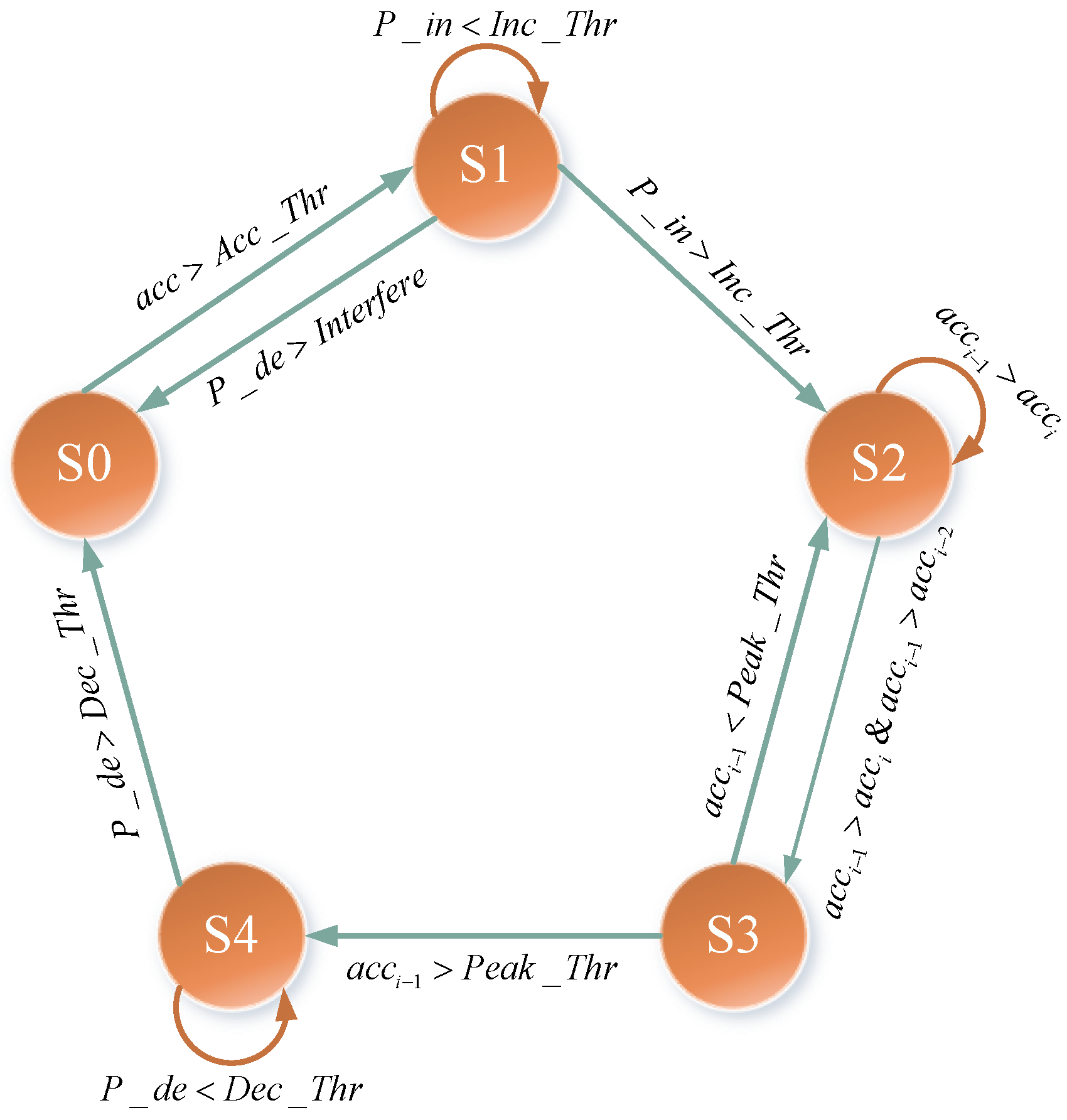
The IFSM gait detection algorithm proposed in this paper consists of five states, denoted as S0–S4, which form a gait cycle corresponding to the walking acceleration waveforms, one by one. The current gait state flows between these five states, and the state flow is completed one step at a time. Since the waveform follows a pattern of “increase–peak–decline–valley “, S0 is defined as the stable state in the transition stage, where the previous step has ended but the next step has not yet started; S1 is defined as the rising state, which means that when the user starts to move, the heel rises gradually and the acceleration increases continuously; S2 represents the state of searching for the peak, i.e., searching for the existing peak after entering the rising state; S3 is set as the peak threshold judgment stage, where the peak found in the previous step is compared with the minimum threshold of the peak, to remove the false wave peak; S4 is defined as the descending state, indicating the process of gradually retracting the foot after leaving the ground.
The thresholds adopted by the IFSM algorithm are , , , , and . Their respective meanings are as follows:
: The threshold of two adjacent acceleration changes;
: The acceleration threshold of each gait at the beginning of the gait detection process;
: The preset threshold value of rising times in a gait cycle, i.e., the maximum value in the rising state;
: The preset threshold value of descending times in a gait cycle, i.e., the maximum value in descending state;
: Lower boundary threshold of the peak;
: Interference threshold.
In order to describe the rising and falling states of the waveform in the gait cycle, two two-state quantities, i.e., and , are introduced. At the beginning of each gait cycle, and are reset to 0. The updates of and are as follows in Equation (6):
where and , respectively, represent the times when the acceleration’s rise and fall are greater than .
The principle of the gait detection algorithm, based on IFSM, is shown in Figure 5.
The principle of the IFSM algorithm can be described as follows:
- (1)
- At the beginning, it is in a stable state, . If the current acceleration is larger than , it enters the state , and and are set to zero at the same time;
- (2)
- The noise shielding mechanism is introduced in the rising state . If there is substantial noise in the data obtained by the accelerometer, the acceleration waveform will fluctuate violently, i.e., and will increase at the same time. Since is smaller than , it will first meet , and the system will return to the stable state for re-detection;
- (3)
- After entering the rising state, if exceeds , the system will enter the state ;
- (4)
- If is less than the current peak after entering the next state, the system will enter the state , otherwise it will return to state ;
- (5)
- In state , if continues to increase until it is greater than , the system returns to state , and the number of steps increases by 1.
3.2. The Dynamic Model of PDR
The dynamic model of PDR can be obtained by combining a step detection algorithm, based on IFSM, with heading estimation. The state vector is selected as follows:
where and represent the east and north position components, respectively, in the local Cartesian coordinates coordinate system defined in the east-north-up (E-N-U) model; is the step size of the PDR positioning, and is the heading.
In the PDR dynamic model, the propagation of the state vector at time is discrete and nonlinear:
where is a function of the state vector , average angular rate , acceleration , and sampling interval . The is processed by the IFSM gait-detection algorithm.
The step length can be obtained from the characteristics of step frequency and acceleration [30]:
where , and are the linear parameters of the step model; and , computed by Equation (5), are the maximum and minimum values of acceleration modulus, respectively.
The heading is computed using Equation (10) [31]:
where is the gain of a complementary filter, and is the heading obtained by the magnetometer.
Assuming that the initial position of the pedestrian is , the position at the next time point is calculated using the step length and the heading , as shown in Figure 6.
The corresponding positioning change can be expressed as:
where is the position of the step, .
Combining Equations (10) and (11), we obtain a formulation of the dynamic model of PDR as:
3.3. Fusion of a PDR Algorithm with a GNSS System
The integration of PDR and GNSS can deliver better performance by combining their respective characteristics. The detailed process for the integration of GNSS and PDR is as follows. First, GNSS information can provide a relatively accurate initial position for the PDR algorithm. Then, the GNSS positioning results are utilized to correct the PDR, to a certain extent, to reduce the cumulative errors. Meanwhile, the PDR positioning results are used directly to correct the GNSS positioning results in a relatively short time in GNSS areas that are partially denied. The stability of the whole positioning process will be improved through the integration of the two positioning technologies.
The state model is:
where , , , and are independent model noises with zero-mean Gaussian distribution; that is, , , , and .
The observation vector is:
where and are the east coordinate and the north coordinate converted from the longitude and latitude, measured by GNSS using the station center coordinate system. In this paper, the carrier phase-smoothing pseudo-range differential algorithm is used to achieve GNSS positioning. and , respectively, are the step size and heading, measured by the PDR algorithm.
The observation model is:
where , , , are Gaussian white noise; , , , and , which are independent of each other.
Since the state equation is a nonlinear equation group, the state transition matrix is obtained by deriving the state Equation (7), according to the EKF principle [32]:
The Jacobian matrix of the observation equation is:
The EKF algorithm depends on the system model and the statistical distribution of measurement noise. In order to improve the adaptability of the system to the environment, the AEKF algorithm, which adjusts noise parameters adaptively, is designed for the fusion of the PDR and GNSS measurements. Equation (18) is defined to determine whether it is occluded.
where is the position difference of two adjacent steps, measured by GNSS, as shown in Equation (19); is the difference between obtained from Equation (9) and .
, calculated by PDR, is not affected by the sheltered environment. Hence, it can be judged that the signal of GNSS is blocked when is large, as can be seen from Equation (18).
Assuming that satisfies Gaussian distribution, with a zero-mean and a variance of , that is, , its probability density function can be written as:
A threshold can be set according to the empirical value, to judge whether it is currently in the occlusion state. If , it is currently in an occluded state. The evaluation result of Equation (20) is introduced into the EKF algorithm to dynamically adjust the process noise and measurement noise. The expression of noise adjustment is as follows:
where and are the system noise covariance matrix and the measurement noise covariance matrix of the initial process, respectively:
The initial position of the fusion positioning system is provided by GNSS positioning, while the initial covariance matrix is . The initial covariance matrix is defined as:
4. Experimental Results and Analysis
4.1. Experimental Setup
In the experiments, the campus of Southeast University in China is selected as the test site. Data were collected using an HONOR v30pro smartphone, which was carried by users while following a predefined trajectory. The sampling rate of IMU was set to 50 Hz.
The experiment consisted of three parts.
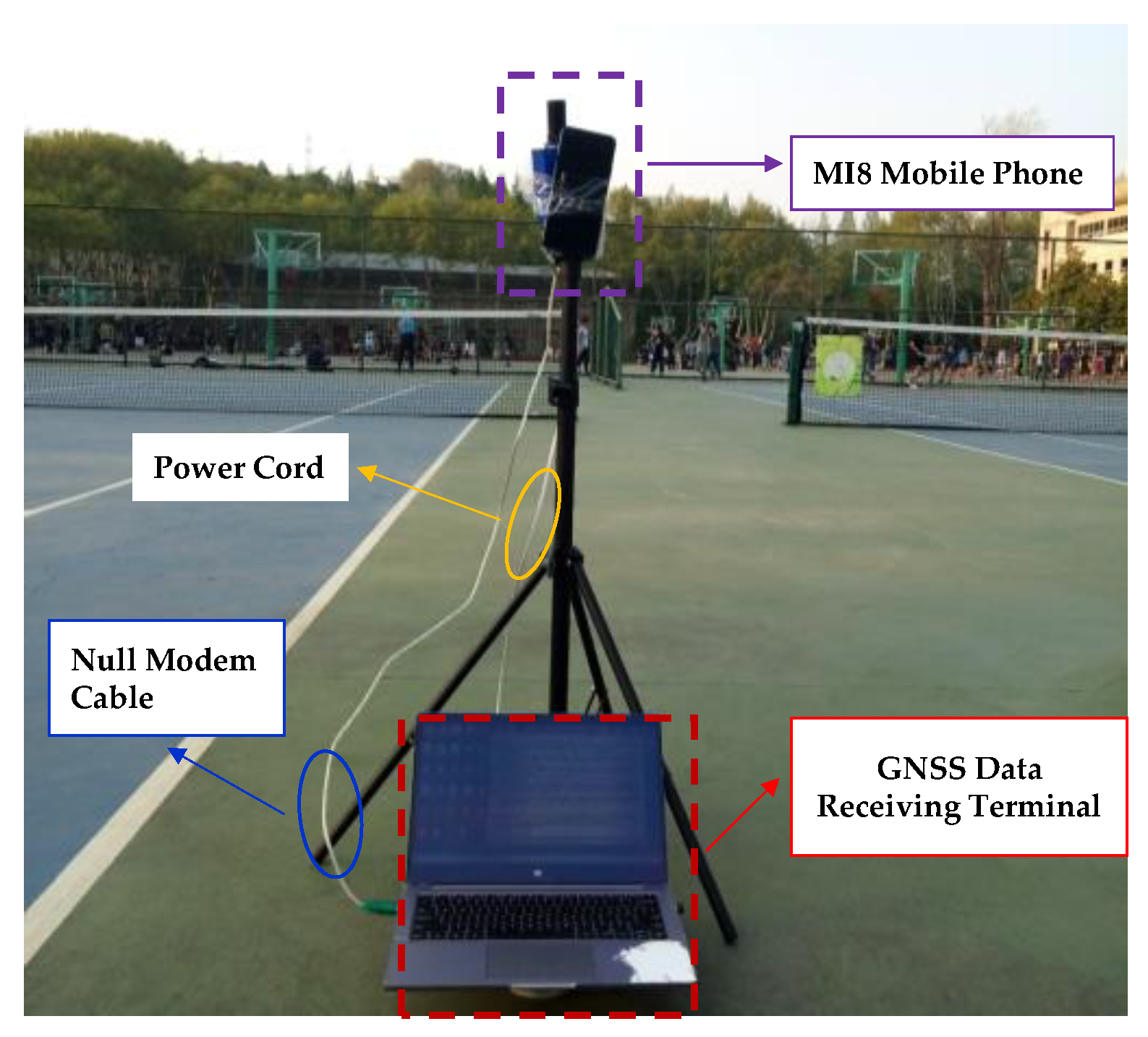
(1) In order to verify the performance of the carrier phase-smoothing pseudo-range algorithm, test experiments were designed. The HONOR v30pro smartphone and the GNSS receiver were placed in the same place for a synchronous observation experiment, as shown in Figure 7. The acquisition time was about 20 min.
(2) The peak detection method and the IFSM algorithm were tested and analyzed for various modes of holding the mobile phone. Five groups of experiments were carried out, namely, normal-speed walking, fast-speed walking, jogging, going upstairs, and going downstairs. Four users with various heights were selected as subjects in each group. In order to avoid contingency, each person was tested 5 times. The mean value of the results of the five experiments was recorded as the number of steps taken by the subjects. In the experiment, the participants were required to walk 60 steps.
(3) The performance of the fusion algorithm was verified by two forms of experimental scenario. The experimental environment of the fountain in Southeast University is shown in Figure 8a, where there is a regular octagon fountain and the surrounding areas are covered with trees. The overview of the “8”-shaped route is shown in Figure 8b, with the walking trajectory marked in a red color. There are buildings and many trees in this scene. The two marked turns are circular arcs. The route, direction, starting points, and reference points of the two experimental scenes are all marked in Figure 8. The test subject was also equipped with a GNSS receiver, which provided a truth reference for the walking trajectory. For all experiments, we focused on phone positions, the subject holding a phone placed in front of his chest.
4.2. Performance Analysis of GNSS Positioning
The positioning accuracy of a smartphone under the three positioning schemes is listed in Table 2. It can be seen from Table 2 that the error of the pseudo-range single point in E and N directions is about 5 m, but the elevation error is up to 10 m. The error of pseudo-range differential positioning is less than that of single-point positioning. The phase-smoothing pseudo-range differential positioning error is the smallest, and the error in the E and N directions is less than 2 m, while the error in the elevation direction is also reduced. Figure 9 shows the positioning error of pseudo-range single-point positioning, pseudo-range difference, and carrier phase smoothing pseudo-range difference in the E, N, and U directions. It can be seen from these figures that the pseudo-range single-point scheme has the largest positioning error and largest noise value; the precision of pseudo-range differential positioning is better than that of pseudo-range single-point positioning, but there is still a large noise value in the N and U directions; compared with the above two kinds of positioning, the noise of carrier-phase smoothing pseudo-range difference is relatively small, showing a relatively smooth accuracy curve with fewer epochs. The pseudo-range difference can effectively eliminate the systematic error of pseudo-range single-point positioning, and the positioning error is reduced. The carrier smoothing of the pseudo-range difference is adopted to ensure the smooth continuity of data.
4.3. Performance Analysis of the IFSM Algorithm
The accuracy of step counting (denoted as ) is defined as follows:
where is the detected steps and is the true number of steps.
The peak detection and the IFSM algorithm are applied to step-counting, as shown in Figure 10. The error of step counting is plotted in Figure 11. The step-counting accuracy of all the algorithms is shown in Figure 12. The gait detection results of two algorithms under different motion states are depicted in Table 3.
From Figure 10, Figure 11 and Figure 12 and Table 3, we observe that the success rates of two gait detection algorithms are more than 96% for the normal-speed and fast-speed gaits of users. The success rates increase to 99% for the IFSM algorithm, based on the detected steps compared with true steps. In the jogging state, the frequency of the smartphone’s swinging with the arm is high. The acceleration at this time is the sum of the acceleration of the user and the swing acceleration of the arm. Therefore, the success rate of the two algorithms is lower than that in the other states. However, the successful detection rates of the IFSM algorithm remain above 97%. For the upstairs and downstairs movements of users, the success rates of the IFSM algorithm are more than 98%, which is significantly higher than with the peak detection method.
4.4. Performance Analysis of the OBPDR Method
The performance of the OBPDR method is evaluated in this experiment. Our proposed methodology fuses the information from PDR, utilizing the IFSM algorithm and GNSS, and enhances the adaptability of the system to the environment, utilizing the AEKF algorithm. In order to verify the performance of the OBPDR method, we compare this method with the other three methods: (1) separate PDR based on IFSM, known merely as IFSM; (2) separate GNSS, known merely as GNSS; (3) the combination of IFSM and GNSS based on EKF, which is known as IFSM/EKF.
4.4.1. Analysis of the Results of the Fountain Experiment
The path length in the fountain experiment is about 113 m. The walking direction is clockwise. The real number of steps is 176, as recorded by one user. The gait detection results based on the IFSM algorithm are shown in Figure 13a, where the red circle indicates that a new step is detected. The estimated heading angle at each step is shown in Figure 13b.
It can be seen from Figure 13a that the number of red circles is 176, that is, the number of steps based on the IFSM algorithm is 176. Compared with the actual number of steps, the accuracy reaches nearly 100%. It is obvious from Figure 13b that the heading angle has fluctuated slightly eight times in terms of straight-line motions.
The positioning results of the fountain experiment are shown in Figure 14. The red line represents the real track (the positioning result of the GNSS receiver). The yellow line stands for the result of IFSM. The green line demonstrates the GNSS positioning result, based on Android. The blue line represents the result of IFSM/EKF, and the black line represents the results of the OBPDR method.
It can be seen from Figure 14 that the true value trajectory is a regular octagon. The IFSM positioning result is relatively smooth, and the deviation from the actual position is small over a short time. However, with an increase in distance, some drift occurs after reference point 5, especially in the last two sections. This is caused by the accumulated error of the inertial sensor, while the uncertainty of the initial value makes it difficult for the PDR to return to the correct track. From the GNSS positioning based on Android phones, it can be seen that the GNSS positioning effect in a shaded environment is quite different from that in open and unobstructed environments. Some periods witness weak signal continuity and jumping, which leads to a divergence in positioning. This indicates that a certain degree of multipath interference is imposed on GNSS signals by the shielding of the surrounding environment, such as trees and buildings, weakening the continuity of the collected GNSS signals. The IFSM/EKF result demonstrates that the location data are not affected by the cumulative error of PDR. The performance of IFSM/EKF is obviously improved by the OBARS method, keeping the location results near the true trajectory.
According to the reference points set in Figure 8a, the errors for each reference point in the fountain experiment are counted, as shown in Table 4. To analyze and compare more intuitively the positioning performance of IFSM, GNSS, IFSM/EKF, and the OBPDR method, a histogram of the error results of each reference point is shown in Figure 15.
4.4.2. Analysis of the Results of the Shade Experiment
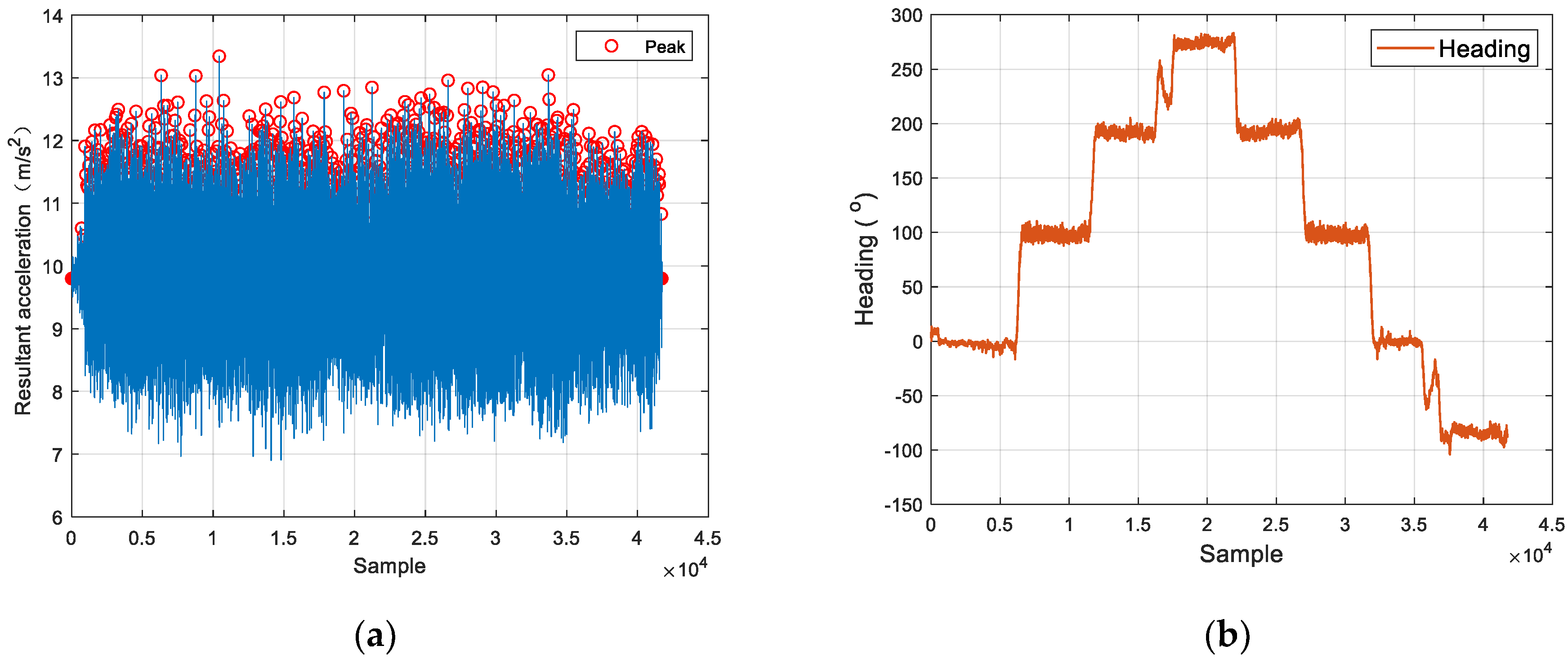
Data are collected according to the planned experimental route: 1-2-3-4-5-6-7-8-9-10-11 in Figure 8b. The length of the shaded lawn path is about 420 m. The walking direction is clockwise. The actual number of steps is 650. The gait detection results, based on the IFSM algorithm, are shown in Figure 16a. The estimated heading angle at each step is shown in Figure 16b.
The results of gait detection based on IFSM, as proposed in this paper, are 651 steps, as shown in Figure 16a. It is obvious from Figure 16b that the heading angle has fluctuated seven times, and there are two sharp spikes, which are two arc-shaped turning points. The heading angles of other sections have small fluctuations.
The positioning results based on Android phones are shown in Figure 17. The true-value track with the GNSS receiver is represented by a red line, with high positioning accuracy. The GNSS receiver performs well in terms of positioning at two circular turns. The IFSM positioning results are represented by the yellow line. The GNSS positioning results, based on Android phones, are represented by green lines. The blue line indicates the location of IFSM/EKF, and the black line represents the location result using the OBPDR method.
It can be seen from Figure 17 that positioning based on IFSM can accurately reflect the “8”-shaped track of pedestrian motion, along with the situation at the two arc-shaped turnings. However, there are still errors in terms of course estimation. As time goes on, the distance error accumulates more and more notably. The regional positioning error within the first 200 m was less than 4 m, while the maximum deviation in the next 200 m was up to 9 m. The GNSS positioning result, based on Android phones, shows that the shaded area has a significant impact on GNSS signals, causing many divergent GNSS signals in terms of continuous motion and low positioning density. In some areas, it is even so severe that no signal can be received at all, resulting in a poor positioning effect. The error remains within 10 m in a shaded environment. The results of the IFSM/EKF tests show that except for the poorly reported effect at two arc turns, the rest of the results can reflect the walking track in a more comprehensive and detailed way. It can be seen that the trajectory, including two arc turns, when using the OBPSR method is closer to the real trajectory. Additionally, in the signal-blocking area, the positioning track remains stable and continuous, and the start and end points are closed well, almost at the same position.
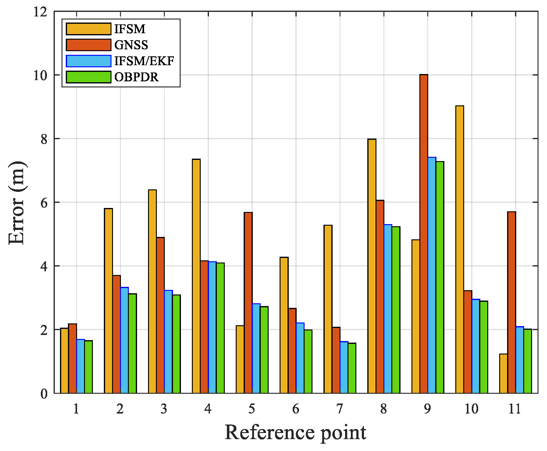
To further analyze the positioning error of each reference point when using the three methods, the table and histogram of error statistics for each reference point in the shaded environment are illustrated in Table 5 and Figure 18.
From Table 5 and Figure 18, it is clear that the maximum positioning error of IFSM at reference point 10 reaches 9 m. In addition, the GNSS positioning is poor, mainly due to the shelter given by trees and buildings. The positioning error at reference point 9 is as high as 10 m, and at other reference point intervals, the positioning error is between 2 and 6 m. The error of IFSM and the OBPDR method at each reference point are relatively stable. The maximum error of the OBPDR method is 0.13 lower than that of the IFSM/EKF. At other reference points, the error with the OBPDR method is also lower than that of IFSM/EKF. Thus, the OBPDR method outperforms IFSM/EKF.
To sum up, compared with IFSM, GNSS, and IFSM/EKF, the positioning accuracy of the OBPDR method improves by 36.7% and 30%. In a shaded environment, where the GNSS signal remains weak, the OBPDR method corrects the severe error caused by point drift and divergence and the large cumulative error caused by IFSM positioning.
5. Conclusions
In this paper, the OBPDR method, which is specific to smartphones, is proposed and consists of the following three steps. Firstly, a novel gait-detection method, based on IFSM, is designed to solve the existing problems of traditional peak detection methods, such as a low gait-recognition rate, poor universality, and poor stability. The proposed IFSM divides a gait cycle into five states and introduces the difference between adjacent acceleration and the threshold of upstairs/downstairs times. To verify the effectiveness of the step-counting of the algorithm, the peak detection method and the IFSM are compared and analyzed from the point of view of different modes of motion and ways of holding mobile phones. The experimental results indicate that the recognition accuracy of IFSM gait detection is higher than that of peak detection. The recognition accuracy was also maintained at between 97.5 and 98.5%. Secondly, the PDR dynamic model can be obtained by combining the IFSM algorithm with the heading estimation. Lastly, the measurements of GNSS are fused to the PDR algorithm, based on the AEKF algorithm, in order to reduce the cumulative error of PDR. Compared with the EKF, this algorithm can enhance the adaptability of the system to the environment. The results of experiments involving different environments show that the accuracy of the OBPDR method is higher than that of IFSM, GNSS, and IFSM/EKF, and the average position error decreased by more than 67.25%. In the future, we hope to apply the method proposed in this paper to the positioning of smartphones in various complex environments.
Author Contributions
R.Z. and J.M. conducted the research; J.M. revised the paper and guided the research. J.L. was responsible for the collection of data and creating the Figures. Q.W. revised and improved the paper. All authors have read and agreed to the published version of the manuscript.
Funding
This work was supported by the projects of the National Key Research and Development Plan of China (No. 2020YFB1600703).
Data Availability Statement
The datasets used and/or analyzed during the current study are available from the corresponding author, on reasonable request.
Conflicts of Interest
The authors declare no conflict of interest.
References
- Kuptametee, C.; Aunsri, N. A review of resampling techniques in particle filtering framework. Measurement 2022, 193, 110836. [Google Scholar] [CrossRef]
- Wu, B.; Ma, C.; Poslad, S.; Selviah, D.R. An Adaptive Human Activity-Aided Hand-Held Smartphone-Based Pedestrian Dead Reckoning Positioning System. Remote Sens. 2021, 13, 2137. [Google Scholar] [CrossRef]
- Yang, H.; Vijayakumar, P.; Shen, J.; Gupta, B.B. A location-based privacy-preserving oblivious sharing scheme for indoor navigation. Future Gener. Comput. Syst. 2022, 137, 42–52. [Google Scholar] [CrossRef]
- Ashraf, I.; Hur, S.; Park, Y. Smartphone sensor based indoor positioning: Current status, opportunities, and future challenges. Electronics 2020, 9, 891. [Google Scholar] [CrossRef]
- Guo, G.; Chen, R.; Ye, F.; Chen, L.; Pan, Y.; Liu, M.; Cao, Z. A Pose Awareness Solution for Estimating Pedestrian Walking Speed. Remote Sens. 2019, 11, 55. [Google Scholar] [CrossRef] [Green Version]
- Yu, J.; Na, Z.; Liu, X.; Deng, Z. WiFi/PDR-integrated indoor localization using unconstrained smartphones. EURASIP J. Wirel. Commun. Netw. 2019, 2019, 3728127. [Google Scholar] [CrossRef]
- Ye, J.; Li, Y.; Luo, H.; Wang, J.; Chen, W.; Zhang, Q. Hybrid urban canyon pedestrian navigation scheme combined PDR, GNSS and beacon based on smartphone. Remote Sens. 2019, 11, 2174. [Google Scholar] [CrossRef] [Green Version]
- Li, X.; Wang, J.; Liu, C. A Bluetooth/PDR integration algorithm for an indoor positioning system. Sensors 2015, 15, 24862–24885. [Google Scholar] [CrossRef] [Green Version]
- Zhu, F.; Tao, X.; Liu, W.; Shi, X.; Wang, F.; Zhang, X. Walker: Continuous and precise navigation by fusing GNSS and MEMS in smartphone chipsets for pedestrians. Remote Sens. 2019, 11, 139. [Google Scholar] [CrossRef] [Green Version]
- Kuang, J.; Niu, X.; Chen, X. Robust pedestrian dead reckoning based on MEMS-IMU for smartphones. Sensors 2018, 18, 1391. [Google Scholar] [CrossRef]
- Huang, L.; Li, H.; Yu, B.; Gan, X.; Wang, B.; Li, Y.; Zhu, R. Combination of smartphone MEMS sensors and environmental prior information for pedestrian indoor positioning. Sensors 2020, 20, 2263. [Google Scholar] [CrossRef] [PubMed] [Green Version]
- Kang, X.; Huang, B.; Qi, G. A novel walking detection and step counting algorithm using unconstrained smartphones. Sensors 2018, 18, 297. [Google Scholar] [CrossRef] [PubMed] [Green Version]
- Park, S.Y.; Heo, S.J.; Park, C.G. Accelerometer-based smartphone step detection using machine learning technique. In Proceedings of the 2017 International Electrical Engineering Congress (iEECON), Pattaya, Thailand, 8–10 March 2017; pp. 1–4. [Google Scholar]
- Wang, X.; Chen, G.; Yang, M.; Jin, S. A multi-mode PDR perception and positioning system assisted by map matching and particle filtering. ISPRS Int. J. Geo-Inf. 2020, 9, 93. [Google Scholar] [CrossRef] [Green Version]
- Chen, Z.; Zou, H.; Jiang, H.; Zhu, Q.; Soh, Y.C.; Xie, L. Fusion of WiFi, smartphone sensors and landmarks using the Kalman filter for indoor localization. Sensors 2015, 15, 715–732. [Google Scholar] [CrossRef]
- Sun, M.; Wang, Y.; Xu, S.; Qi, H.; Hu, X. Indoor positioning tightly coupled Wi-Fi FTM ranging and PDR based on the extended Kalman filter for smartphones. IEEE Access 2020, 8, 49671–49684. [Google Scholar] [CrossRef]
- Pan, M.-S.; Lin, H.-W. A step counting algorithm for smartphone users: Design and implementation. IEEE Sens. J. 2014, 15, 2296–2305. [Google Scholar] [CrossRef]
- Santos, J.; Costa, A.; Nicolau, M.J. Autocorrelation analysis of accelerometer signal to detect and count steps of smartphone users. In Proceedings of the 2019 International Conference on Indoor Positioning and Indoor Navigation (IPIN), Pisa, Italy, 30 September–3 October 2019; pp. 1–7. [Google Scholar]
- Chen, G.; Meng, X.; Wang, Y.; Zhang, Y.; Tian, P.; Yang, H. Integrated WiFi/PDR/Smartphone using an unscented kalman filter algorithm for 3D indoor localization. Sensors 2015, 15, 24595–24614. [Google Scholar] [CrossRef] [Green Version]
- Wang, M.; Duan, N.; Zhou, Z.; Zheng, F.; Qiu, H.; Li, X.; Zhang, G. Indoor PDR positioning assisted by acoustic source localization, and pedestrian movement behavior recognition, using a dual-microphone smartphone. Wirel. Commun. Mobile Comput. 2021, 2021, 9981802. [Google Scholar] [CrossRef]
- Abdi, A.; Barger, J.A.; Kaveh, M. A parametric model for the distribution of the angle of arrival and the associated correlation function and power spectrum at the mobile station. IEEE Trans. Veh. Technol. 2002, 51, 425–434. [Google Scholar] [CrossRef] [Green Version]
- Alzantot, M.; Youssef, M. UPTIME: Ubiquitous pedestrian tracking using mobile phones. In Proceedings of the 2012 IEEE Wireless Communications and Networking Conference (WCNC), Paris, France, 1–4 April 2012; pp. 3204–3209. [Google Scholar] [CrossRef]
- Wang, G.H.; Liang, J.Z.; Chen, J.; Zhu, X.J. Acceleration Difference Finite State Machine Step Algorithm. Comput. Sci. Explor. 2016, 10, 1133–1142. [Google Scholar] [CrossRef]
- Yu, Y.; Chen, R.; Chen, L.; Li, W.; Wu, Y.; Zhou, H. Autonomous 3D indoor localization based on crowdsourced Wi-Fi fingerprinting and MEMS sensors. IEEE Sens. J. 2021, 22, 5248–5259. [Google Scholar] [CrossRef]
- Arpaia, P.; Buzio, M.; Di Capua, V.; Grassini, S.; Parvis, M.; Pentella, M. Drift-Free Integration in Inductive Magnetic Field Measurements Achieved by Kalman Filtering. Sensors 2021, 22, 182. [Google Scholar] [CrossRef] [PubMed]
- Chattha, M.; Naqvi, I.H. Pilot: A precise IMU based localization technique for smart phone users. In Proceedings of the 2016 IEEE 84th Vehicular Technology Conference (VTC-Fall), Montréal, QC, Canada, 18–21 September 2016; pp. 1–5. [Google Scholar] [CrossRef]
- Xie, D.; Jiang, J.; Wu, J.; Yan, P.; Tang, Y.; Zhang, C.; Liu, J. A Robust GNSS/PDR Integration Scheme with GRU-Based Zero-Velocity Detection for Mass-Pedestrians. Remote Sens. 2022, 14, 300. [Google Scholar] [CrossRef]
- Kaczmarek, A.; Rohm, W.; Klingbeil, L.; Tchórzewski, J. Experimental 2D extended Kalman filter sensor fusion for low-cost GNSS/IMU/Odometers precise positioning system. Measurement 2022, 193, 110963. [Google Scholar] [CrossRef]
- Ba, Z.; Zheng, T.; Zhang, X.; Qin, Z.; Li, B.; Liu, X.; Ren, K. Learning-based Practical Smartphone Eavesdropping with Built-in Accelerometer. In Proceedings of the NDSS 2020, San Diego, CA, USA, 23–26 February 2020. [Google Scholar]
- Hobara, H.; Saito, S.; Hashizume, S.; Sakata, H.; Kobayashi, Y. Individual Step Characteristics During Sprinting in Unilateral Transtibial Amputees. J. Appl. Biomech. 2018, 34, 509–513. [Google Scholar] [CrossRef]
- Thio, V.; Ånonsen, K.B.; Bekkeng, J.K. Relative heading estimation for pedestrians based on the gravity vector. IEEE Sens. J. 2021, 21, 8218–8225. [Google Scholar] [CrossRef]
- Honglong, C.; Liang, X.; Chengyu, J.; Kraft, M.; Weizheng, Y. Combining Numerous Uncorrelated MEMS Gyroscopes for Accuracy Improvement Based on an Optimal Kalman Filter. IEEE Trans. Instrum. Meas. 2012, 61, 3084–3093. [Google Scholar] [CrossRef]
Figure 1.
The flow chart of the PDR algorithm.

Figure 2.
The walking components of pedestrian movement.

Figure 3.
Results diagram of the triaxial acceleration signal.

Figure 4.
Acceleration signal preprocessing.

Figure 5.
The gait detection algorithm, based on IFSM.

Figure 6.
The schematic diagram of PDR.

Figure 7.
GNSS positioning experiment scenario.

Figure 8.
The experimental test scenarios. (a) The experimental environment of a fountain; (b) the experimental route under a shading environment.
Figure 8.
The experimental test scenarios. (a) The experimental environment of a fountain; (b) the experimental route under a shading environment.

Figure 9.
The GNSS positioning error. (a) Pseudo-range single-point positioning; (b) pseudo-range differential positioning; (c) carrier-smoothed pseudo-range differential location.
Figure 9.
The GNSS positioning error. (a) Pseudo-range single-point positioning; (b) pseudo-range differential positioning; (c) carrier-smoothed pseudo-range differential location.

Figure 10.
The comparison of gait detection.

Figure 11.
The error of gait detection.

Figure 12.
The successful rate of gait detection.

Figure 13.
The PDR information in the fountain experiment environment. (a) The results of gait detection, based on the IFSM algorithm; (b) the estimations of the heading angle.
Figure 13.
The PDR information in the fountain experiment environment. (a) The results of gait detection, based on the IFSM algorithm; (b) the estimations of the heading angle.

Figure 14.
The positioning results of fountain experiment.

Figure 15.
The statistical results of position errors in fountain experiment.

Figure 16.
The PDR information in the shade experiment environment. (a) The results of gait detection, based on the IFSM algorithm; (b) the estimation of the heading angle.
Figure 16.
The PDR information in the shade experiment environment. (a) The results of gait detection, based on the IFSM algorithm; (b) the estimation of the heading angle.

Figure 17.
The positioning results of shadow experiment.

Figure 18.
The statistical results of position errors in shadow experiment.


Table 1.
Empirical parameters in the gait-detection algorithm.
| Threshold Name | Symbol | |
|---|---|---|
| Two adjacent acceleration change thresholds | 0.04 | |
| Gait onset acceleration threshold | 9.8 | |
| Rising state maximum | 6 | |
| Falling state maximum | 6 | |
| Lower bound threshold of wave crest | 10.5 | |
| Interference shielding threshold | 3 |
Table 2.
Statistics of GNSS positioning error.
| Scheme | E(m) | N(m) | U(m) |
|---|---|---|---|
| Pseudo range single point positioning | 1.08 | 1.13 | 1.25 |
| Pseudo range differential positioning | 2.21 | 1.38 | 1.15 |
| Phase smoothed pseudo-range difference | 1.67 | 4.51 | 1.92 |
Table 3.
Gait detection results of 20 experiments under different motion states.
| Motion State | Experimental Subjects | Peak Detection Method | Improved FSM Method | ||
|---|---|---|---|---|---|
| Result (Step) | Accuracy | Result (Step) | Accuracy | ||
| Normal-speed walking | A | 58.9 | 98.1% | 60.5 | 99.2% |
| B | 59.2 | 98.6% | 60.5 | 99.2% | |
| C | 59.0 | 98.3% | 60.3 | 99.5% | |
| D | 58.7 | 97.8% | 60.2 | 99.6% | |
| Fast-speed walking | A | 57.6 | 96.0% | 60.3 | 99.5% |
| B | 58.4 | 97.3% | 60.4 | 99.3% | |
| C | 58.2 | 97.0% | 59.8 | 99.6% | |
| D | 58.3 | 97.1% | 60.1 | 99.8% | |
| Jogging | A | 56.1 | 93.5% | 61.1 | 98.1% |
| B | 55.3 | 92.1% | 61.5 | 97.5% | |
| C | 56.0 | 93.3% | 61.8 | 97.1% | |
| D | 55.7 | 92.8% | 60.5 | 99.3% | |
| Upstairs | A | 58.1 | 96.8% | 60.9 | 98.3% |
| B | 58.0 | 96.6% | 59.6 | 99.3% | |
| C | 57.6 | 96.0% | 60.4 | 99.3% | |
| D | 57.7 | 96.1% | 59.6 | 99.3% | |
| Downstairs | A | 58.0 | 96.6% | 60.9 | 98.5% |
| B | 58.3 | 97.1% | 61.1 | 98.1% | |
| C | 57.5 | 95.8% | 59.9 | 99.8% | |
| D | 57.3 | 95.5% | 59.9 | 98.8% | |
Table 4.
Statistics of reference point errors in fountain experiments.
| Reference Point | IFSM (m) | GNSS (m) | IFSM/EKF(m) | OBPDR (m) |
|---|---|---|---|---|
| 1 | 1.08 | 1.13 | 1.25 | 1.24 |
| 2 | 2.21 | 1.38 | 1.15 | 1.12 |
| 3 | 1.67 | 4.51 | 1.92 | 1.81 |
| 4 | 2.01 | 3.42 | 2.20 | 2.15 |
| 5 | 1.68 | 3.55 | 1.60 | 1.57 |
| 6 | 2.59 | 5.63 | 2.15 | 2.12 |
| 7 | 5.40 | 2.46 | 3.03 | 2.99 |
| 8 | 11.03 | 1.25 | 1.65 | 1.64 |
| 9 | 11.16 | 1.17 | 1.18 | 1.17 |
Table 5.
Statistics of reference-point errors in shade experiments.
| Reference Point | IFSM (m) | GNSS (m) | IFSM/EKF(m) | OBPDR (m) |
|---|---|---|---|---|
| 1 | 2.04 | 2.18 | 1.69 | 1.65 |
| 2 | 5.80 | 3.70 | 3.32 | 3.12 |
| 3 | 6.39 | 4.89 | 3.23 | 3.09 |
| 4 | 7.35 | 4.16 | 4.13 | 3.99 |
| 5 | 2.12 | 5.68 | 2.81 | 2.72 |
| 6 | 4.27 | 2.66 | 2.21 | 1.99 |
| 7 | 5.28 | 2.07 | 1.65 | 1.57 |
| 8 | 7.98 | 6.06 | 5.30 | 5.23 |
| 9 | 4.82 | 10.01 | 7.41 | 7.28 |
| 10 | 9.03 | 3.22 | 2.95 | 2.89 |
| 11 | 1.23 | 5.70 | 2.09 | 2.01 |
Publisher’s Note: MDPI stays neutral with regard to jurisdictional claims in published maps and institutional affiliations. |
© 2022 by the authors. Licensee MDPI, Basel, Switzerland. This article is an open access article distributed under the terms and conditions of the Creative Commons Attribution (CC BY) license (https://creativecommons.org/licenses/by/4.0/).
Share and Cite
MDPI and ACS Style
Zhang, R.; Mi, J.; Li, J.; Wang, Q. A Continuous PDR and GNSS Fusing Algorithm for Smartphone Positioning. Remote Sens. 2022, 14, 5171. https://0-doi-org.brum.beds.ac.uk/10.3390/rs14205171
AMA Style
Zhang R, Mi J, Li J, Wang Q. A Continuous PDR and GNSS Fusing Algorithm for Smartphone Positioning. Remote Sensing. 2022; 14(20):5171. https://0-doi-org.brum.beds.ac.uk/10.3390/rs14205171
Chicago/Turabian StyleZhang, Rui, Jing Mi, Jing Li, and Qing Wang. 2022. "A Continuous PDR and GNSS Fusing Algorithm for Smartphone Positioning" Remote Sensing 14, no. 20: 5171. https://0-doi-org.brum.beds.ac.uk/10.3390/rs14205171
Note that from the first issue of 2016, this journal uses article numbers instead of page numbers. See further details here.