Terrestrial Laser Scanning in Assessing the Effect of Different Thinning Treatments on the Competition of Scots Pine (Pinus sylvestris L.) Forests

Abstract

Thinning is a forest management activity that regulates the competition between the trees within a forest. However, the effect of different thinning treatments on competition is largely unexplored, especially because of the difficulty in measuring crown characteristics. This study aimed to investigate how different type and intensity thinning treatments affect the stem- and crown-based competition of trees based on terrestrial laser scanning (TLS) point clouds. The research was conducted in three study sites in southern Finland where the Scots pine (Pinus sylvestris L.) is the dominant tree species. Nine rectangular sample plots of varying sizes (1000 m² to 1200 m²) were established within each study site, resulting in 27 sample plots in total. The experimental design of each study site included two levels of thinning intensities and three thinning types, resulting in six different thinning treatments. To assess the competition between the trees, six distance-dependent competition indices were computed for each tree. The indices were based on diameter at breast height (DBH) (CI_DBH), height (CI_H), maximum crown diameter (CI_MCD), crown projection area (CI_CA), crown volume (CI_CV), and crown surface area (CI_CS). The results showed that for both moderate and intensive intensities, the competition decrease was 45.5–82.5% for thinning from below, 15.6–73.6% for thinning from above, and 12.8–66.8% for systematic thinning when compared with control plots. In most cases, the crown- and stem-based metrics were affected by thinning treatments significantly when compared with control plots at a 95% confidence interval. Moreover, moderate from-below and from-above thinning showed no statistical difference with each other in both crown- and stem-based competition indices except for CI_DBH (p-value ≤ 0.05). Our results confirm the great potential of TLS point clouds in quantifying stem- and crown-based competition between trees, which could be beneficial for enhancing ecological knowledge on how trees grow in response to competition.

1. Introduction

Growth is one of the important ecological processes that closely interact with and respond to the local environment of trees within forest stands. It is the main driver of tree structure at any given time [1]. The limited amount of sufficient growth resources such as light, soil nutrients, water, temperature, and growing space leads to increasing competition between trees [2,3,4,5]. Hence, different levels of competition will cause variation in tree growth [6] due to the individual ability of trees to respond to their local environment with structural changes [1]. Overall, there are two types of size-symmetric or asymmetric competitions that are defined based on resource acquisitions. Size-symmetric competition occurs when the competitive effect is proportional to some measure of size, while in asymmetric competition larger trees obtain a disproportionate share of resources [7,8,9]. Competition plays a crucial role in determining tree size, especially diameter, height, and crown attributes as a neighborhood process [10,11]. So, it is effective in the individual tree structure and forest dynamics [10]. In forest stands, the competition caused by the neighboring trees can be characterized quantitatively by calculating different kinds of competition indices (CIs) [12]. Generally, CIs of individual trees are categorized into two main groups: distance-dependent [13,14] and distance-independent [15,16,17]. Distance-dependent indices quantify competition by considering the distance between a subject tree and its neighbors, whereas distance-independent indices do not need tree individual locations [16]. Distance-dependent indices may meet the requirements for presenting a more trustworthy estimation of the growth of individual trees [14,18]. In addition, they are considered the distance from a subject tree to its neighbor trees that can quantify the value of competition on a fine scale [3]. The use of CIs has been improving the ability to simulate the response of individual trees to silvicultural treatments [16]. Especially, by increasing the effects of global warming and loss of biodiversity, more attention has been paid to diverse silvicultural treatments.

In forestry, thinning is the most substantial silvicultural treatment that decreases the competition within neighborhood trees by reducing the tree density (i.e., trees/ha) [19,20]. As a result, the remaining trees uptake more available resources for promoting individual tree growth [21]. In fact, controlling the competition among individual trees by reducing tree density is the main goal of various thinning treatments [22]. Thinning treatments have different effects on growth and yield, wood quality, mortality, and ecological functions (i.e., understory vegetation, nutrient cycle, etc.) [21,23]. There are some studies that have used traditional forest mensuration methods to examine the effects of thinning treatments on growth and yield [1,24,25], stand stability [21,26], adaptiveness to droughts [27,28,29], evaporation [30,31], provision of ecosystem services [32,33,34,35], carbon and nutrients [36,37], and even biodiversity [38,39] at both the tree and stand levels. However, mapping trees is a labor-intensive task, and it is a key aspect of the computation of distance-dependent CIs. These methods are costly and only applicable on small scales. Moreover, they concentrate on easy-to-measure parameters such as diameter at breast height (DBH), while crown characteristics are critical in quantifying the tree’s response to thinning and spacing [40,41]. In contrast, airborne laser scanning data have been found to be effective in individual tree-level analysis and crown characterization [42,43,44,45]. Moreover, close-range terrestrial laser scanning (TLS) data can even provide millimeter-level details on the tree’s structure, including stem forms, branches, and various crown characteristics using millions to billions of 3D points [46,47]. Their effectiveness has been proved in the prediction of forest structure attributes [48,49,50]. Moreover, with the ability to create tree maps, CIs can be predicted by TLS data efficiently [3,51,52,53,54,55]. Moreover, they provide a reliable solution for forest monitoring by collecting explicit in situ information [56]. For instance, Saarinen et al. [57] have assessed the effects of thinning treatment on stem growth allocation of individual Scots pine trees using TLS. They showed that the size and shape of individual Scots pine trees are affected by different thinning types and intensities. Calder et al. [56] concluded that TLS is a viable alternative to the traditional forest mensuration methods for collecting tree and forest characteristics such as crown attributes and spatial distribution.

Therefore, this study aimed to investigate how different type and intensity thinning treatments affect the stem and crown competition of trees based on terrestrial laser scanning point clouds. It is hypothesized that the removal of large trees (i.e., thinning from above) will reduce the competition more than the removal of smaller trees (i.e., thinning from below) (H1), systematic thinning from above has no difference in competition with thinning from above (H2), and higher intensity thinning decreases the competition increasing growth space (i.e., distance to the closest neighboring trees) (H3). Two different types of CIs were considered based on 1) DBH (CI_DBH) and height (CI_H) and 2) maximum crown diameter (CI_MCD), crown projection area (CI_CA), crown volume (CI_CV), and crown surface area (CI_CS). We focused on Scots pine (Pinus sylvestris L.) stands subjected to different thinning types (i.e., from below (or low thinning), from above (or crown thinning), and systematic) and intensities (i.e., moderate and intensive).

2. Materials and Methods

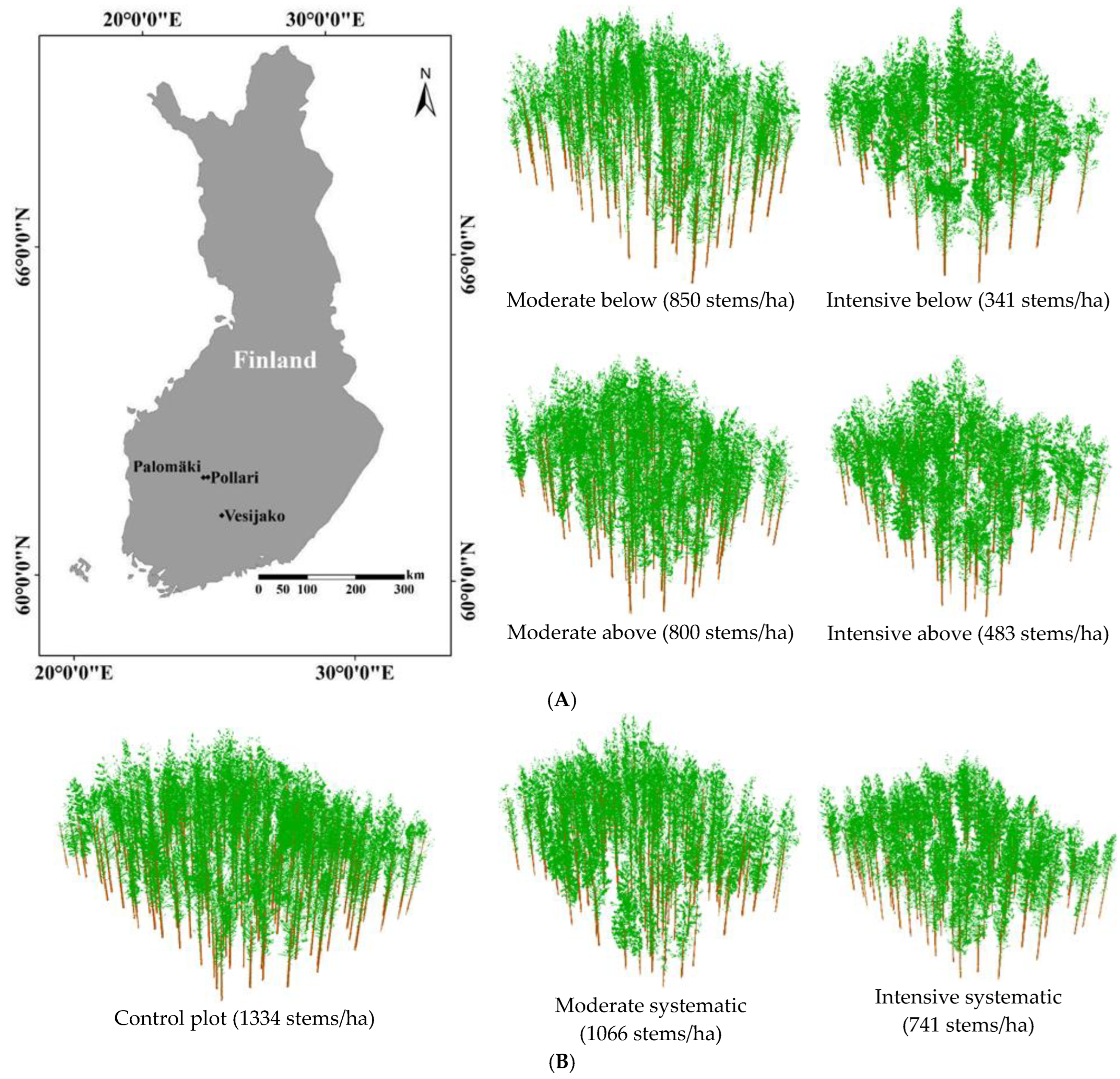
2.1. Study Site

This study was conducted in three sites including Vesijako (61°21.8′N 25°6.3′E), Pollari (62°4.4′N 24°30.1′E), and Palomäki (62°3.6′N 24°19.9′E), located in the southern boreal forest zone (Figure 1A). These study sites were established and are managed by the Natural Resources Institute Finland (Luke). Experiments to investigate the effect of different thinning treatments in the Scots pine dominant stands were established in 2006 in Pollari and Vesijako, whereas experiments in Palomäki were established in 2005. All experiments are considered even aged, and the age at the time of establishment was about 50 years. They are also characterized as mesic heath forests (i.e., Myrtillus forest site type according to a theory by A. K. Cajander [58]). The mean elevation above sea level in Vesijako, Pollari, and Palomäki is 120 m, 155 m, and 135 m, respectively (characterized as flat), with respective temperature sums of 1256, 1130, and 1195 days.

2.2. Designing Thinning Experiments

Nine rectangular sample plots were established with varying sizes (1000 m² to 1200 m²) for each study site in 2005–2006, resulting in 27 sample plots in total. The experimental design for each study site included two levels of thinning intensity and three thinning types, resulting in six different thinning treatments (Figure 1B), namely: (I) moderate thinning from below (3 plots), (II) intensive thinning from below (3 plots), (III) moderate thinning from above (4 plots), (IV) intensive thinning from above (4 plots), (V) moderate systematic thinning from above (5 plots), and (VI) intensive systematic thinning from above (5 plots). Moreover, one control plot for each study site (3 plots in total) was established without thinning treatment (un-thinned sample plots). The exact location of each sample plot had been recorded by VRS-corrected GNSS. Duration after the thinning treatments and the period for competition response on the remaining individual trees was 12 years in Pollari and Vesijako study sites and 13 years in Palomäki. According to the latest field inventory campaign that was carried out from autumn 2018 to spring 2019, there were 2102 individual trees in all 27 plots. Plot-level comparison of different thinning treatments characteristics including control plots before thinning treatments (2005–2006), after thinning treatments (2005–2006), and after growth period (2018–2019) has been provided in

Table 1. Mean plot-level characteristics before thinning treatments (2005–2006), after thinning treatments (2005–2006), and after growth period (2018–2019). G = basal area (m²/ha), N = stem number per hectare, V = volume (m³/ha), D_w = mean diameter weighted by basal area (cm), H_w = mean height weighted by basal area (m).

Before Thinning (2005–2006)
	No Treatment	Thinning from Below (Moderate/Intensive)	Thinning from Above (Moderate/Intensive)	Systematic Thinning (Moderate/Intensive)
G (m2/ha)	27.6	26.9/26.9	27.8/24.7	25.4/26.0
N/ha	1336	1285/1260	1417/1201	1256/1218
V (m3/ha)	224.4	215.4/216.6	216.9/191.0	199.7/210.6
Dw (cm)	17.8	17.5/18.0	17.3/17.6	17.5/18.0
Hw (m)	16.1	16.1/16.3	15.9/15.6	15.9/16.2
After thinning (2005–2006)
	No Treatment	Thinning from Below (Moderate/Intensive)	Thinning from Above (Moderate/Intensive)	Systematic Thinning (Moderate/Intensive)
G (m2/ha)	27.6	18.3/8.9	18.5/9.1	18.2/8.7
N/ha	1336	719/292	955/479	988/522
V (m3/ha)	224.4	148.8/72.9	144.0/69.1	141.3/67.3
Dw (cm)	17.8	18.7/20.4	16.9/16.5	16.5/15.7
Hw (m)	16.1	16.5/16.9	15.7/15.3	15.6/15.5
After growth period (2018–2019)
	No Treatment	Thinning from Below (Moderate/Intensive)	Thinning from Above (Moderate/Intensive)	Systematic Thinning (Moderate/Intensive)
G (m2/ha)	37.1	28.4/15.9	28.3/16.1	27.6/15.9
N/ha	1249	705/286	915/446	937/466
V (m3/ha)	380.3	291.8/160.8	282.3/150.5	267.9/150.4
Dw (cm)	21.2	23.5/27.5	21.2/22.3	20.7/22.2
Hw (m)	21.3	21.7/21.6	21.0/19.5	20.3/20.0

.

The three thinning types involved different methods for selecting the trees to be removed. In thinning from above, mostly dominant trees were removed, whereas in thinning from below suppressed and co-dominant trees were removed. In both thinning from above and from below, small and damaged (e.g., forked, crooked) trees were removed, and the regular spatial distribution of the remaining trees was pursued. In systematic thinning from above, only dominant trees were removed while small and suppressed trees were left to grow. Moreover, the regularity of spatial distribution of remaining individual trees was not underlined, although large gaps were avoided. However, large canopy gaps were avoided. The intensity of thinning represents the proportion of the basal area that was removed by a thinning treatment. After the moderate thinning intensity, approximately 68% of the stocked stand basal area remained. Respectively, after the intensive thinning intensity, approximately 34% of the stocked stand basal areas remained compared to the basal area before the thinning.

2.3. Terrestrial Laser Scanning Point Cloud Data

TLS point cloud data were acquired with a Trimble TX5 3D phase-shift laser scanner for all three study sites between September and October 2018. The used scanner works at a 905 nm wavelength and measures up to 976,000 points per second with a beam divergence of 0.19 m rad. One scan covers 360 degrees horizontally and 300 degrees vertically. A multi-scan approach was used in the TLS data acquisition to ensure that all of the trees were characterized by the point clouds. That is, the scanner was placed, and the point clouds collected from eight different scan locations evenly distributed around each of the sample plots. Two of the scan locations (i.e., center scans) were placed near the center of the sample plot a few meters apart from each other while the remaining six scan locations (i.e., auxiliary scans) were distributed evenly around the sample plot, preferring locations near the plot borders. In each scan location, the scanner was placed on a tripod at the height of approximately 1.6–1.8 m. Point clouds from different scan locations were registered and merged together using artificial reference targets (i.e., constant-sized white spheres with a diameter of 198 mm attached to tripods). It was carried out in the FARO Scene software with a mean distance error of 2.9 mm, mean vertical error of 2.3 mm, and mean horizontal error of 1.3 mm [57]. Point clouds from different scan locations were registered together using artificial reference targets (i.e., white spheres with a diameter of 198 mm) attached to tripods and distributed around the sample plot. With the applied scan setup, most of the trees became scanned from multiple directions, enabling geometrically accurate 3D reconstruction of the tree structures using the obtained multi-scan point clouds. The maximum horizontal distance between a scanner and a tree was approximately 7 m, at which distance the applied scanning parameters resulted in a point spacing of 2.7 mm in a single scan point cloud. Considering the fact that, in the registered multi-scan point cloud, point clouds from individual scans were overlapping, and that mostly the trees were located closer to the scanners, the resulting point cloud featured a point spacing of a few millimeters. Depending on the structure of a sample plot, the obtained overall point density was 52,000–91,000 points/m².

2.3.1. Deriving Individual Tree Structural Metrics from Point Clouds

An automatic workflow was adopted to segment individual trees, classify point clouds into stem and non-stem points, and estimate tree metrics that is explained in detail.

First, registered multi-scan point cloud data were segmented into individual trees using raster-based canopy segmentation method. Topography removal workflow presented by Ritter et al. [59] was used to obtain height-normalized point cloud data, which were further used for generating canopy height models (CHMs) with 20 cm resolution in LAStools software (Rapidlasso GmbH, Gilching, Germany) [60]. A Variable Window Filter approach was applied to obtain the preliminary location of treetops [61]. Then, CHMs were segmented into individual tree crowns using a marker-controlled watershed segmentation [62]. The obtained individual tree crown segments were used in a point-in-polygon approach applied to the XY plane to extract the initial set of points belonging to the individual tree. Out of 2102 trees, 2076 (98.8%) were detected automatically by TLS data. Notably, no significant difference at 95% confidence interval was achieved in completeness of tree detection in different thinning treatments including control plot [2].

Second, the initial set of points for each tree was then further classified into stem points and non-stem points using an algorithm developed by Yrttimaa et al. [2] and available in Yrttimaa [63]. It is based on a general assumption that stem points have more planar, vertical, and cylindrical characteristics than points representing branches and foliage [64]. The algorithm acts from tree stem towards top of the tree by partitioning individual trees point clouds into different bins of 0–4 m to access stem origin and others 0.5 m bin afterwards until reaching to the treetop. Then, an iterative process is employed in each point clouds bin including grid average down-sampling, surface normal filtering, point cloud clustering, and RANSAC-cylinder filtering to identify the distinguishing features separating stem points from foliage points (see Yrttimaa et al. [2] for more details).

Third, after completing point cloud classification, seven metrics characterizing the structure of the stem and crown of individual trees were computed from the classified stem and non-stem point clouds, respectively. They are diameter at breast height (DBH), the height of trees (H), maximum crown diameter (MCD), crown projection area (CA), crown volume (CV), and crown surface area (CS) (

Table 2. Stem and crown metrics were extracted from TLS point clouds.

Metric (Unit)	Description/Calculation
XY Location (m)	Center of a vertical cylinder fitted into stem points around the breast height
DBH (cm)	Diameter at breast height (1.3 m) of the individual trees obtained from taper curve
Height (m)	The maximum height of individual tree point cloud
Maximum crown diameter (m)	Maximum crown diameter based on the 2D convex hull
Crown projection area (m2)	Area of the crown 2D convex hull projected onto XY plane
Crown volume (m3)	Volume of the 3D convex hull enveloping crown points
Crown surface area (m2)	Surface area enveloping crown points based on the 3D convex hull

).

Tree stem metrics, namely DBH and tree height (H), were obtained from the classified stem points following the procedure originally presented in Yrttimaa et al. [64]. H was determined as the vertical distance between the highest and lowest points for each tree. A taper curve (i.e., stem diameter as a function of tree height) was obtained for stem characterization by first dividing the stem points into horizontal point cloud slices at 10 cm intervals and then estimating the diameter of each stem section through circle fitting. Cubic spline smoothing was applied to these diameter-height observations to remove false observations and to interpolate missing observations as proposed in Saarinen et al. [65]. DBH was then obtained from the point-cloud-based taper curve as a diameter at 1.3 m height. XY location was determined as the center of a vertical cylinder fitted into stem points around the breast height. The RMSE of TLS-derived height and DBH was 0.89–2.22 and 0.63–0.76 cm in different thinning treatments including control plot. Additionally, field-measured and TLS estimates of H and DBH were in similar distribution regardless of applied thinning treatments [2].

Crown metrics, namely MCD, CA, CV, and CS, were computed from non-stem individual tree point clouds using the rLiDAR package of R [66]. To accomplish this, 2D convex hull was applied by identifying the crown point clouds lying on the 2D convex hull, and CA was measured. Moreover, MCW was obtained as a distance between two outer points in the XY plane [57], whereas 3D convex hull by applying Delaunay triangulations to the outer points of the closed convex surfaces boundary of crown point clouds was used to derive CV and CS [67].

Table 3. Minimum (Min), maximum (Max), mean, and standard deviation (Std) of the terrestrial laser scanning (TLS) measurements for diameter at breast height (DBH), height (H), maximum crown diameter (MCD), crown projection area (CA), crown volume (CV), and crown surface area (CS) for each thinning treatment.

TLS Metrics	Statistics	No Treatment	Thinning from Below (Moderate/Intensive)	Thinning from Above (Moderate/Intensive)	Systematic Thinning (Moderate/Intensive)
DBH (cm)	Min	8	12.6/17.9	9.6/13.4	7.5/10.9
	Mean	18.6	22.1/3	19.2/20.9	18.7/20.2
	Max	33.7	33.2/36.3	31.3/30.8	32.9/30.4
	Std	4.8	3.5/3.8	4.1/3.3	4.1/4.1
H (m)	Min	3.6	3.9/17.4	15.1/15.1	8.4/13.4
	Mean	19.7	20.7/20.8	20.1/18.8	19.2/18.5
	Max	28.3	25.7/25.2	25.4/23.2	25.6/23.7
	Std	3	2.1/1.9	1.6/1.6	2.2/2.5
MCD (m)	Min	0.7	1/3	1.2/2.1	0.5/1.5
	Mean	3.1	3.9/5.1	3.5/4.1	3.5/3.9
	Max	6.7	6.5/7.5	6.4/6	7.1/7.1
	Std	0.9	1.1/0.9	0.9/0.7	1/0.8
CA (m2)	Min	0.2	1/6.8	1/3.9	1/1.8
	Mean	6.4	10.8/18.2	8.9/12	8.3/11
	Max	25.4	24.7/42.4	24.8/25	27.7/29.7
	Std	3.6	5.3/6.2	4.5/4.8	4.4/4.7
CV (m3)	Min	0.67	1/46.2	5.5/24.6	1/10.2
	Mean	54.3	89.56/150.6	69.1/85.7	63.9/78.9
	Max	22.8	224.46/366.3	221.3/181.8	214.9/232.6
	Std	34.9	47.16/58.2	37.9/34.5	36.7/39.5
CS (m2)	Min	8.6	1/87.2	30.1/61.7	4/38.9
	Mean	100.5	131.1/171.1	113/120.8	106.3/115
	Max	231.4	229.2/287.8	227.3/192.9	211.5/2
	Std	38.4	41.7/38.3	34.9/27.9	35.8/35.8

summarizes the descriptive statistics of the TLS-derived metrics characterizing the structure of the stems and crowns.

2.3.2. Computation of Competition Indices

Considering the ability of TLS data in providing tree maps, the distance-dependent competition indices (CIs) can be quantified in an easier way than traditional field measurements. They are well-known indices to count competition status based on the size and distance of the neighbors. Hegyi equation [61] is one of them that could present different combinations of tree characteristics. Moreover, it is easy to compute while explaining variation in growth within the similar level of accuracy than other indices [16]. For this reason, we applied the Hegyi equation [68] using the stem metrics of DBH and H and crown metrics of MCD, CA, CV, and CA (Equation (1)). CIs were computed for all the trees in the original rectangular sample plots by a fixed 8 m search radius around the subject tree. The 8 m search radius has been suggested by previous studies [13,69,70]. If all trees within the original plot would be included, the competition evaluation for trees at the outer edge of the plots would have been insufficient due to the lack of data outside of the plot. Therefore, to reduce the edge effect, a circular plot of the 11 m radius was placed at the center of the original plots, and trees within that were included in the analyses, resulting in 720 trees (

Table 4. Summary statistics of sample trees in each treatment measured by TLS data.

Attribute	Statistics	No Treatment n = 129	Thinning from Below		Thinning from Above		Systematic Thinning
			Moderate n = 76	Intensive n = 34	Moderate n = 141	Intensive n = 62	Moderate n = 183	Intensive n = 95
DBH (cm)	Min	9.75	14.25	17.9	11	14.3	9	11.75
	Mean	16.56	21.77	26.19	19.05	21.87	19.03	21.1
	Max	34.4	31.35	34.65	32.25	28.35	28.8	29.1
	Std	4.76	3.81	4.04	4.15	2.96	3.74	3.96
H (m)	Min	14.94	16.98	18.2	16.7	14.9	13.7	13.9
	Mean	20.76	21.13	21.18	20.38	19.28	19.7	19.14
	Max	30.3	25.2	24.8	24.7	22.7	24.9	23.3
	Std	3.06	2.24	1.66	1.47	1.49	1.85	2.24
Volume (m3)	Min	0.06	0.13	0.23	0.08	0.12	0.04	0.07
	Mean	0.33	0.39	0.56	0.3	0.36	0.29	0.34
	Max	1.27	0.89	1.03	0.92	0.66	0.73	0.72
	Std	0.2	0.16	0.19	0.14	0.11	0.12	0.14

).

$$CI={\displaystyle \sum }_{i=1}^n X_i/\left(X\times dis{t}_i\right)$$

(1)

Here, CI is the competition index for an individual tree; n refers to number of neighbors within the 8 m radius search; $X_i$ is considered structural metrics (i.e., DBH, H, MCD, CA, CV, and CS) of the ith neighbor tree, X refers to structural metrics of the subject tree; $dis{t}_i$ is horizontal distance from the subject tree to ith neighbor tree (m). Relative differences (%) were determined by subtracting the mean of competition estimated in thinned plots from the mean of competition estimated in control plots and dividing the result of subtraction with the mean competition index of control plots and multiplying by 100.

2.4. Statistical Analyses

To examine whether competition indices are different between thinning treatments, a mixed effect model was used. It is useful in analyzing multiple observations that are usually correlated within independent sampling units [71]. As we conducted different thinning treatments in multiple plots at three study sites, a nested two-level linear mixed-effects model fitted using Restricted Maximum Likelihood included in package nlme of the R-software was used [72] (Equation (2)):

$$\begin{gathered} y_{ij}={\beta }_{1}No treatmen{t}_1+{\beta }_{2}Moderate belo{w}_i+{\beta }_{3}Intensive belo{w}_i \\ \hspace{1em}\hspace{1em}\hspace{1em}\hspace{1em}\hspace{1em}\hspace{1em}\hspace{1em}\begin{array}{l}+{\beta }_{4}Moderate abov{e}_i+{\beta }_{5}Intensive abov{e}_i\\ +{\beta }_{6}Moderate systemati{c}_i+{\beta }_{7}Intensivesy stemati{c}_i+{\alpha }_i+c_{ij}\\ +{\in }_{ij}\end{array} \end{gathered}$$

(2)

where $y_{ij}$ is each competition index at a time, ${\beta }_1$, …, ${\beta }_7$ refers to fixed parameters, I, i = 1, …, M, are study site, j = 1, …, $n_i$, refers to a sample plot, ${\alpha }_i$ and $c_{ij}$ are normally distributed random effects for study site i and sample plot j within study site i, respectively, with mean zero and unknown, unrestricted variance–covariance matrix, and ${\in }_{ij}$ is a residual error with mean zero and unknown variance. Tukey’s honest significance test was used for revealing the statistically significant difference in the CIs affected by the different thinning treatments.

3. Results

3.1. Descriptive Statistics

Table 5. Minimum (Min), mean, maximum (Max), and standard deviation (Std) and relative difference (bolded, in brackets) of competition indices among thinning treatments. CI_DBH = competition index based on DBH, CI_H = competition index based on height, CI_MCD = competition index based on maximum crown diameter, CI_CA = competition index based on crown projection area, CI_CV = competition index based on crown volume, CI_CS = competition index based on crown surface area.

Competition Index	Statistics	No Treatment	Thinning from Below (Moderate/Intensive)	Thinning from Above (Moderate/Intensive)	Systematic Thinning (Moderate/Intensive)
CIDBH	Min	2	1.3/0.3	1.7/0.7	1.5/0.5
	Mean/ (Relative difference)	5.5	2.6 (52.7%)/ 1 (82.5%)	4.1 (25%)/ 1.5 (73.2%)	4.2 (24.2%)/ 1.8 (66.8%)
	Max	10.7	4.6/1.4	9.8/2.6	9.8/5.3
	Std	1.8	0.6/0.3	1.7/0.4	1.4/0.9
CIH	Min	2.4	1.4/0.3	2.1/0.7	1.8/0.5
	Mean (Relative difference)	5.2	2.5 (50.7%)/ 0.9 (81.6%)	4 (23%)/ 1.5 (71.2%)	4.1 (21.3%)/ 1.8 (64.9%)
	Max	7.6	4.1/1.4	7.3/2.4	8.1/4.2
	Std	1.1	0.6/0.2	1.3/0.4	0.9/0.8
CIMCD	Min	1.8	1.3/0.3	1.5/0.6	1.5/0.4
	Mean (Relative difference)	5.2	2.7 (49.2%)/ 1 (82%)	4.2 (19.5%)/ 1.5 (72%)	4.2 (18.9%)/ 1.8 (64.7%)
	Max	10.3	5.1/1.7	10.7/2.7	10.4/5.4
	Std	1.7	1/0.3	1.9/0.4	1.5/0.9
CICA	Min	1.1	1/0.3	1.1/0.4	1/0.4
	Mean (Relative difference)	5.6	3.1 (45.5%)/ 1.1 (81.3%)	4.7 (15.6%)/ 1.5 (73.1%)	4.9 (12.8%)/ 2 (64.1%)
	Max	15.9	11.3/3	15/3.2	15/8.3
	Std	3	2/0.5	2.9/0.6	2.8/1.3
CICV	Min	1.2	1/0.3	1.2/0.4	1/0.4
	Mean (Relative difference)	5.8	3.1 (46.3%)/ 1.1 (81.7%)	5 (16.3%)/ 1.5 (73.6%)	5.1 (13.3%)/ 2.1 (63.2%)
	Max	17.7	12.2/3.2	18.6/3.4	17.1/9.6
	Std	3.3	2.2/0.6	3.1/0.7	3.1/1.6
CICS	Min	1.8	1.3/0.3	1.7/0.6	1.4/0.5
	Mean (Relative difference)	5.2	2.7 (48.3%)/ 1 (80.8%)	4.2 (19.3%)/ 1.5 (71.5%)	4.2 (18%)/ 1.9 (63.1%)
	Max	11.1	6.4/2	10/2.6	9.7/6.4
	Std	1.8	1/0.4	1.8/0.5	1.6/1.1

shows the statistics related to CIs in different types and intensities of thinning treatments when compared with control plots. Generally, the competition decreased for all different treatment types ranging by 12.8–52.7% in moderate thinning and 63.1–82.5% in intensive thinning. The mentioned decreasing trend was observed for both crown- and stem-level CIs.

Intensive thinning from below followed by intensive thinning from above mainly resulted in smaller mean and standard deviation compared to the other thinning treatments with different types and intensities (Table 5). It was 50.7% to 52.7% in moderate and 81.6% to 82.5% in intensive intensities of thinning from below for stem-based competitions (Figure 2 and Table 5), while the reduction in stem-based CIs was 23% to 25% and between 71.2% and 73.2% for moderate and intensive thinning from above, respectively. The maximum decrease in crown-based CIs was 82% for CI_MCD with implementing intensive thinning from below. Our results showed that the decrease in crown-based competition by implementing moderate from-below thinning ranged from 45.5% to 49.2%, while it was 15.6% to 19.5% for moderate from above. Intensive systematic thinning treatment resulted in a decrease in CI_DBH by 66.8% and in CI_H by 64.9%. It was 24.2% and 21.3% in moderate systematic thinning, respectively. The standard deviation (Std.) of crown metrics for intensive systematic thinning treatment was 0.9 to 1.6, while it was higher for moderate intensity with a Std. of 1.5 to 3.1. Notably, systematic treatment and thinning from above with moderate intensities mainly resulted in a similar level of competition when compared with control plots in terms of mean and standard deviation (Table 5).

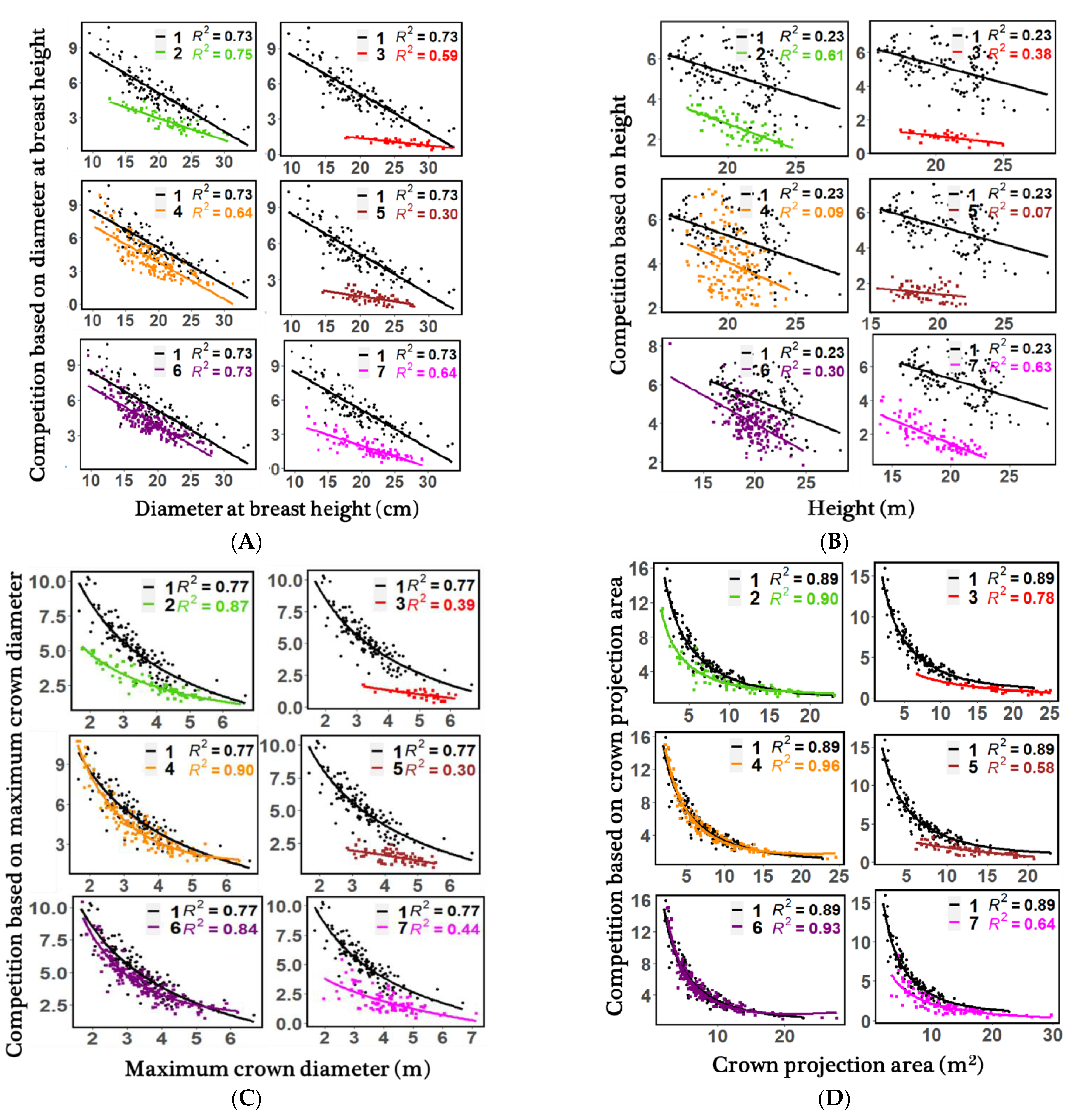
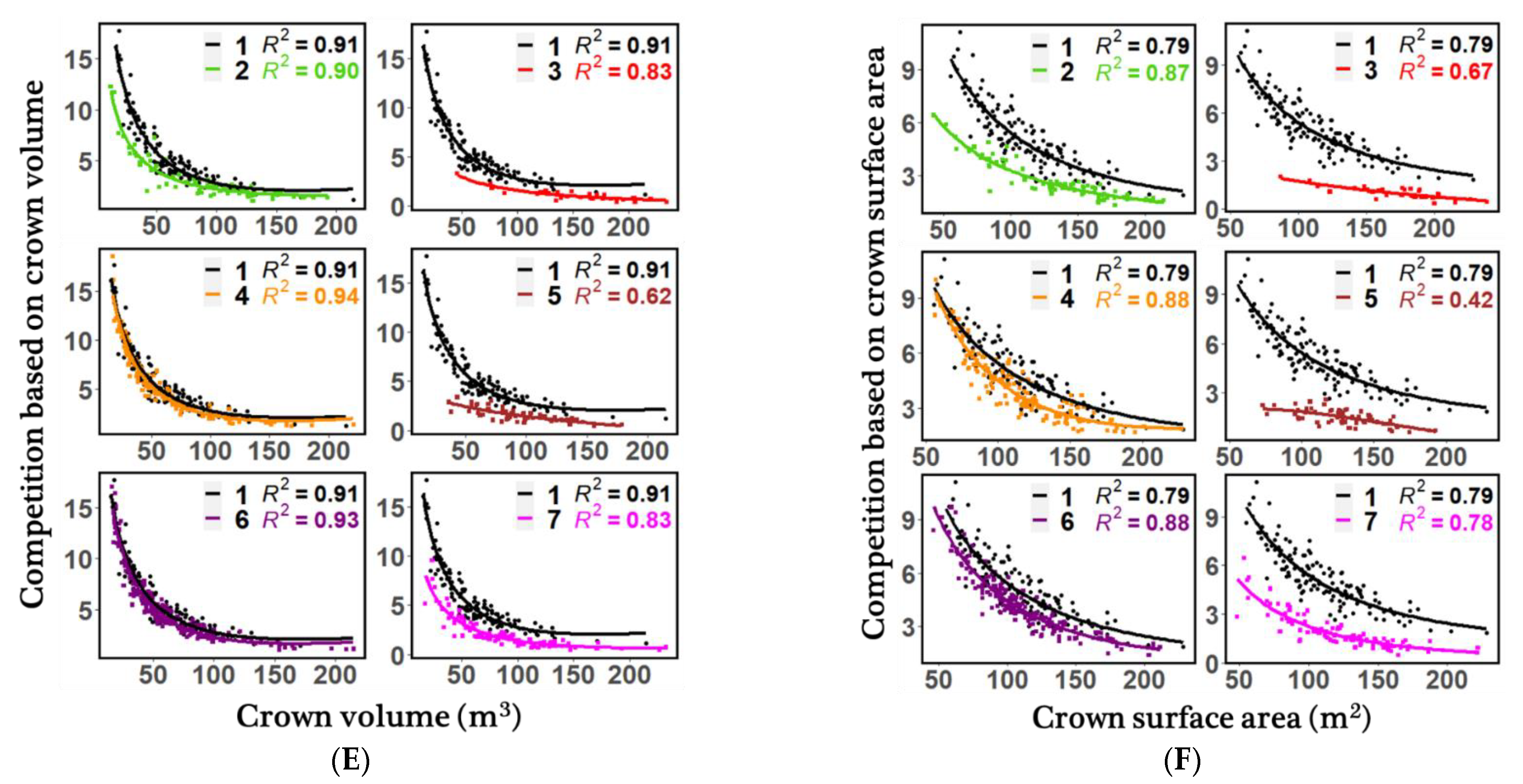
3.2. Individual Tree Competitiveness

Understanding the relationship between competition around the target tree and its size can provide additional insights into the internal tree competitiveness in different thinning treatments. The relationship between CIs against the stem and crown size metrics for all thinning treatments is provided in Figure 3. Generally, there is an inverse relationship between measured stem and crown size of trees and the CIs based on them. This means that there is less competition around a big tree and vice versa. In addition, the results showed that intensive thinning treatments led to notable competition reduction, especially intensive thinning from below. So, the effect of internal tree size was less visible. It could be explained that lower competition tended to increase the growth of the trees in size of stem and crown compared to control plots in intensive thinnings (Figure 3A–F). As shown, sample plots with moderate treatments tend to have more similar trends with control plots when compared with intensive treatments.

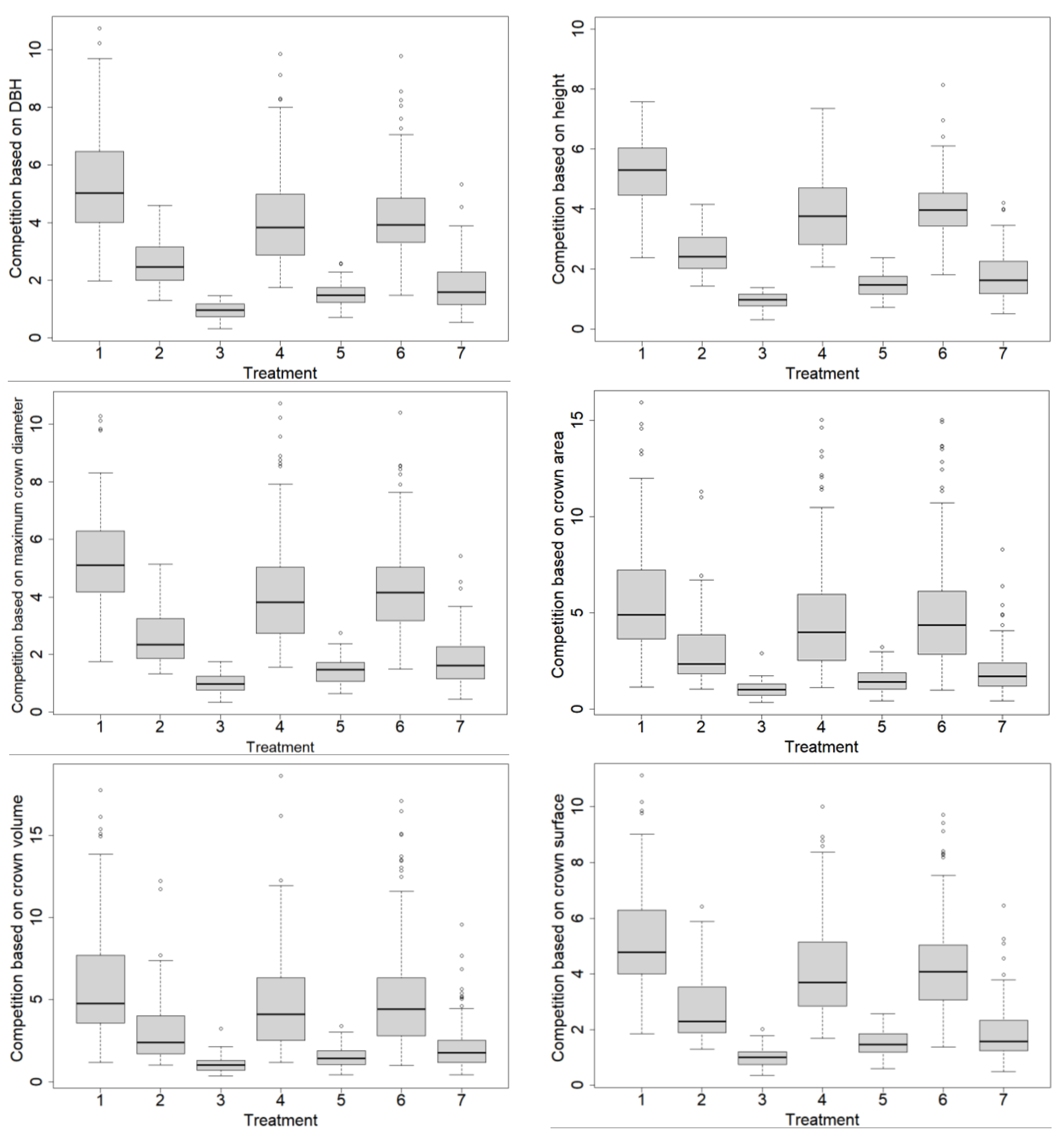
3.3. The Effect of Thinning Treatments on CIs

The results of the nested two-level linear mixed-effect model representing quantitative details of differences in CIs between different thinning treatments and intensities have been reported in

Table 6. Statistically significant difference (p-value ≤ 0.05) was caused by different thinning treatments based on Tukey’s honest significance test. CI_DBH = competition index based on DBH, CI_H = competition index based on height, CI_MCD = competition index based on maximum crown diameter, CI_CA = competition index based on crown projection area, CI_CV = competition index based on crown volume, CI_CS = competition index based on crown surface area.

Compared Competition Indices Caused by the Thinning Treatments		Competition Indices with Statistically Significant Difference (p ≤ 0.05)
Moderate below	No Treatment	CIDBH, CIH, CIMCD, CICA, CICV, CICS
Intensive below	No Treatment	CIDBH, CIH, CIMCD, CICA, CICV, CICS
Moderate above	No Treatment	CIDBH, CIH,
Intensive above	No Treatment	CIDBH, CIH, CIMCD, CICA, CICV, CICS
Moderate systematic	No Treatment	-
Intensive systematic	No Treatment	CIDBH, CIH, CIMCD, CICA, CICV, CICS
Intensive below	Moderate below	CIDBH, CIH
Moderate above	Moderate below	CIDBH
Moderate systematic	Moderate below	CIDBH, CIH, CIMCD, CICA, CICV, CICS
Intensive above	Intensive below	-
Intensive systematic	Intensive below	-
Intensive above	Moderate above	CIDBH, CIH, CIMCD, CICA, CICV, CICS
Moderate systematic	Moderate above	-
Intensive systematic	Intensive above	-
Intensive systematic	Moderate systematic	CIDBH, CIH, CIMCD, CICA, CICV, CICS

. The moderate and intensive thinning from below, intensive thinning from above, and intensive systematic thinning had statistically significant differences with control plots in aspects of all crown- and stem-based competitions (p-value ≤ 0.05). Only stem-based CIs in moderate thinning from above were statistically different from control plots at 95% confidence interval, decreasing the CI_DBH by 25% and CI_H by 23%, respectively. There was no statistical difference between control plots and moderate systematic thinning in the aspect of CIs (p-value ≥ 0.05). Different intensities of systematic thinning showed statistically significant differences with each other in all CIs. Intensive intensities in different thinning of systematic and from above, systematic and from below, and from above and from below were observed to be not statistically different. Moderate and intensive thinning from below were statistically different in their stem-based CIs only. In moderate intensity, the thinning from below resulted in significantly smaller CI_DBH than thinning from above (p-value ≤ 0.05), while they showed no statistical difference for other CIs. On the contrary, from below and systematic thinning with moderate intensities resulted in a statistically significant difference for all CIs (Table 6), while the difference between moderate intensities of systematic and from above were statistically insignificant.

4. Discussion

The aim of this study was using the TLS point clouds of trees to investigate how thinning types (i.e., from below, from above, and systematic) with different intensities (i.e., moderate and intensive) were affected in competition among individual Scots pine trees. The competition was the highest in control plots, as could be expected. This is in line with previous studies such as Baniya and Mandal [73] and del Río et al. [21]. It can be explained by tree density leading to excessively diminished space for individual tree growth, resulting in the reduction in tree sizes (Figure 1B) [11,22,57,74,75]. Intensive thinning treatments lead to lower competition compared with moderate thinning treatments. So, the H3 hypothesis was accepted. Thus, we expect higher growth resource availability such as space, nutrients, water, and light in intensive thinning treatments by increasing the growing space around each individual tree [6]. Our results showed that thinning from below greatly reduced the competition when compared with thinning from above and systematic thinning treatments. It led to rejection of the H1 hypothesis. It can be explained by the significant contribution of smaller trees to uptake existing growth resources which were removed in from-below thinning treatment [11]. As a result, other competitors are able to utilize the released growth resources and competition for canopy space occurs less than the competition for water and soil nutrients (i.e., tree crowns vs. root system) [11]. In other words, if root architecture is constant, with the removal of intermediate and suppressed trees, the taller trees can uptake more water and nutrients from the soil [76,77]. Notably, by decreasing the interception as the result of thinning, the available water in the soil will be increased [27]. In contrast, Mäkinen and Isomäki [25] and Pukkala et al. [78], who addressed the effect of thinning on growth, reported that thinning affected co-dominant and medium-sized Scots pine trees more than dominant trees. Similarly, del Rio et al. [79] indicated that in Scots pine stands, after the thinning from below, intermediate (in terms of DBH) individual trees can uptake more released resources than dominant trees. Nevertheless, more caution should be taken in interpreting the results, as the time lag between thinning treatments and TLS measurements in our study was 13 years at most.

When comparing the effects of different thinning treatments on the competition with control plots, all CIs showed a statistically significant difference at a 95% confidence interval, except for moderate systematic thinning (see Table 6). There was no statistically significant decrease in the competition of moderate thinning treatments from above and systematic when compared with each other, i.e., the H2 hypothesis was accepted. It could be caused by the similarity in these treatments in removing larger individual trees [57], due to the moderate intensity of systematic thinning, although it led to more growing space for the remaining trees but could not affect the competition responses to the thinning in individual Scots pine trees. Individual tree crowns are not only the main factor of light penetration in the sub-canopy [80] but also the determinant of seedling and sapling dynamics [81]. Therefore, understating the effect of thinning on competitive interaction among the crown of individual trees is critical. Results of this study indicated that different thinning types tend to decrease the crown competition from 12.8% (moderate systematic thinning) to 82% (intensive thinning from below) in comparison with control plots (see Table 5). It was 45.5% to 49.2% and 15.6% to 19.5% for moderate thinning treatments from below and from above, respectively. When comparing the effects of different thinning treatments on the competition with each other, all CIs showed statistically significant differences, except four thinning treatment pairs. They include the comparison between intensive thinning from below with both of intensive systematic and from-above thinning treatments, comparison between moderate systematic and from-above thinning treatments, and comparison between intensive systematic and from-above thinning treatments (Table 6). It is worth mentioning that from-below thinning with two intensities only differed by CI_DBH and CI_H. Similarly, moderate from-below and from-above thinning treatments showed no statistical difference with each other in both crown- and stem-based CIs, except for CI_DBH.

We evaluated stem- and crown-based TLS-derived competition indices against six management procedures, and significant differences were achieved in competition status of individual trees in the comparison with control plots. However, it should be considered that TLS accuracy in characterizing the 3D structure of a forest depends on multiple factors. Scanning setup, the algorithms used in tree detection and reconstruction of trees, and completeness of point clouds are the main sources of error limiting TLS application in forest measurements [2,82].

Although competition can be reduced by thinning treatments and thus lead to increased tree growth, it must be considered that too intensive thinning treatment may cause undesirable and harmful effects such as low stability of the trees against wind and snow in the early years after the thinning, decreasing in the wood quality and total volume, biodiversity reduction, nutrient budget imbalance, soil erosion, and losing other ecosystem services [21,83,84]. Therefore, despite their permissibility, too intensive thinning treatments are not proposed for the Finnish Scots pine forests. Heavy thinning treatments can be used when forest managers decide to increment the cutting incomes in a short period [83,85].

5. Conclusions

Thinning treatments have different effects on growth and yield, wood quality, mortality, and ecological functions by controlling the competition among individual trees. However, CIs are mainly extracted from easy-to-measure parameters such as DBH and height, while tree crown characteristics are critical in quantifying the tree’s response to thinning. In addition, distance-dependent CIs are rarely studied because of the difficulty in creating tree maps. To fill the mentioned gap, this study aimed to evaluate CIs against management strategies in Scots pine stands using TLS point clouds. Our results demonstrate the effects of different type and intensity thinning treatments on TLS-derived individual tree stem- and crown-based CIs. Intensive thinning from below led to a maximum decrease in competition indices by 82.5% when compared with other treatments. Unlike others, there was no statistical difference between control plots and moderate systematic thinning in the aspect of CIs (p-value ≥ 0.05), although only stem-based CIs in moderate thinning from above were statistically different from control plots at a 95% confidence interval, decreasing the CIDBH by 25% and CIH by 23%, respectively. Moreover, we found no statistically significant decrease in the competition of moderate thinning treatments from above and systematic when compared with each other. This study provides novel insights into forest ecology and management strategies, especially in boreal forests. However, further analysis is needed to understand the contribution of each growth resource on CIs variation under mixed forest stand conditions.

References

1. Lang, A.C.; Härdtle, W.; Bruelheide, H.; Geißler, C.; Nadrowski, K.; Schuldt, A.; Yu, M.; von Oheimb, G. Tree Morphology Responds to Neighbourhood Competition and Slope in Species-Rich Forests of Subtropical China. For. Ecol. Manag. 2010, 260, 1708–1715. [Google Scholar] [CrossRef]
2. Yrttimaa, T.; Saarinen, N.; Kankare, V.; Hynynen, J.; Huuskonen, S.; Holopainen, M.; Hyyppä, J.; Vastaranta, M. Performance of Terrestrial Laser Scanning to Characterize Managed Scots Pine (Pinus Sylvestris L.) Stands Is Dependent on Forest Structural Variation. ISPRS J. Photogramm. Remote Sens. 2020, 168, 277–287. [Google Scholar] [CrossRef]
3. Ma, Q.; Su, Y.; Tao, S.; Guo, Q. Quantifying Individual Tree Growth and Tree Competition Using Bi-Temporal Airborne Laser Scanning Data: A Case Study in the Sierra Nevada Mountains, California. Int. J. Digit. Earth 2018, 11, 485–503. [Google Scholar] [CrossRef]
4. Wainwright, J.; Mulligan, M. (Eds.) Environmental Modelling: Finding Simplicity in Complexity; Wiley and John & Sons: Hoboken, NJ, USA, 2013. [Google Scholar]
5. Perry, D.A. Trees Crop Plants; Institute of Terrestrial Ecology: Kendal, UK, 1985. [Google Scholar]
6. Pretzsch, H. Growing Space and Competitive Situation of Individual Trees. In Forest Dynamics, Growth and Yield; Springer: Berlin/Heidelberg, Germany, 2009; pp. 291–336. [Google Scholar]
7. Cordonnier, T.; Kunstler, G. The Gini Index Brings Asymmetric Competition to Light. Perspect. Plant Ecol. Evol. Syst. 2015, 17, 107–115. [Google Scholar] [CrossRef]
8. Forrester, D.I. Linking Forest Growth with Stand Structure: Tree Size Inequality, Tree Growth or Resource Partitioning and the Asymmetry of Competition. For. Ecol. Manag. 2019, 447, 139–157. [Google Scholar] [CrossRef]
9. Weiner, J. Asymmetric Competition in Plant Populations. Trends Ecol. Evol. 1990, 5, 360–364. [Google Scholar] [CrossRef]
10. Bataineh, M.; Childs, E. Competition Effects on Growth and Crown Dimensions of Shortleaf and Loblolly Pine in Mature, Natural-Origin, Pine–Hardwood Mixtures of the Upper West Gulf Coastal Plain of Arkansas, USA: A Neighborhood Analysis. Forests 2021, 12, 935. [Google Scholar] [CrossRef]
11. Thorpe, H.C.; Astrup, R.; Trowbridge, A.; Coates, K.D. Competition and Tree Crowns: A Neighborhood Analysis of Three Boreal Tree Species. For. Ecol. Manag. 2010, 259, 1586–1596. [Google Scholar] [CrossRef]
12. Pitkänen, T.P.; Bianchi, S.; Kangas, A. Quantifying the Effects of Competition on the Dimensions of Scots Pine and Norway Spruce Crowns. Int. J. Appl. Earth Obs. Geoinf. 2022, 112, 102941. [Google Scholar] [CrossRef]
13. Pont, D.; Dungey, H.S.; Suontama, M.; Stovold, G.T. Spatial Models with Inter-Tree Competition from Airborne Laser Scanning Improve Estimates of Genetic Variance. Front. Plant Sci. 2021, 11, 596315. [Google Scholar] [CrossRef]
14. Versace; Gianelle; Frizzera; Tognetti; Garfì; Dalponte Prediction of Competition Indices in a Norway Spruce and Silver Fir-Dominated Forest Using Lidar Data. Remote Sens. 2019, 11, 2734. [CrossRef] [Green Version]
15. Coonen, E.J.; Sillett, S.C. Separating Effects of Crown Structure and Competition for Light on Trunk Growth of Sequoia Sempervirens. For. Ecol. Manag. 2015, 358, 26–40. [Google Scholar] [CrossRef]
16. Burkhart, H.E.; Tomé, M. Modeling Forest Trees and Stands; Springer: Dordrecht, The Netherlands, 2012; ISBN 978-94-007-1597-4. [Google Scholar]
17. Biging, G.S.; Dobbertin, M. Evaluation of Competition Indices in Individual Tree Growth Models. For. Sci. 1995, 41, 360–377. [Google Scholar]
18. Tomé, M.; Burkhart, H.E. Distance-Dependent Competition Measures for Predicting Growth of Individual Trees. For. Sci. 1989, 35, 816–831. [Google Scholar]
19. Assmann, E. The Principles of Forest Yield Study; Pergamon Press: Oxford, UK, 1970; p. 56. [Google Scholar]
20. Larson, P.R. Formation and Properties of Juvenile Wood in Southern Pines: A Synopsis (Vol. 129); US Department of Agriculture, Forest Service, Forest Products Laboratory: Madison, WI, USA, 2001.
21. Del Río, M.; Bravo-Oviedo, A.; Pretzsch, H.; Löf, M.; Ruiz-Peinado, R. A Review of Thinning Effects on Scots Pine Stands: From Growth and Yield to New Challenges under Global Change. For. Syst. 2017, 26, eR03S. [Google Scholar] [CrossRef]
22. Ashton, M.S.; Kelty, M.J. The Practice of Silviculture: Applied Forest Ecology; Wiley and John & Sons: Hoboken, NJ, USA, 2018. [Google Scholar]
23. Jonard, M.; Misson, L.; Ponette, Q. Long-Term Thinning Effects on the Forest Floor and the Foliar Nutrient Status of Norway Spruce Stands in the Belgian Ardennes. Can. J. For. Res. 2006, 36, 2684–2695. [Google Scholar] [CrossRef]
24. Niemistö, P.; Kilpeläinen, H.; Poutiainen, E. Effect of First Thinning Type and Age on Growth, Stem Quality and Financial Performance of a Scots Pine Stand in Finland. Silva Fenn. 2018, 52, 21. [Google Scholar] [CrossRef] [Green Version]
25. Mäkinen, H.; Isomäki, A. Thinning Intensity and Long-Term Changes in Increment and Stem Form of Norway Spruce Trees. For. Ecol. Manag. 2004, 201, 295–309. [Google Scholar] [CrossRef]
26. Cameron, A.D. Importance of Early Selective Thinning in the Development of Long-Term Stand Stability and Improved Log Quality: A Review. Forestry 2002, 75, 25–35. [Google Scholar] [CrossRef]
27. Ammer, C. Unraveling the Importance of Inter- and Intraspecific Competition for the Adaptation of Forests to Climate Change; Springer: Cham, Switzerland, 2016; pp. 345–367. [Google Scholar]
28. Sohn, J.A.; Saha, S.; Bauhus, J. Potential of Forest Thinning to Mitigate Drought Stress: A Meta-Analysis. For. Ecol. Manag. 2016, 380, 261–273. [Google Scholar] [CrossRef]
29. Giuggiola, A.; Bugmann, H.; Zingg, A.; Dobbertin, M.; Rigling, A. Reduction of Stand Density Increases Drought Resistance in Xeric Scots Pine Forests. For. Ecol. Manag. 2013, 310, 827–835. [Google Scholar] [CrossRef]
30. Boczoń, A. Effect of thinning on evaporation of scots pine forest. Appl. Ecol. Environ. Res. 2016, 14, 367–379. [Google Scholar] [CrossRef]
31. Knoche, D. Effects of Stand Conversion by Thinning and Underplanting on Water and Element Fluxes of a Pine Ecosystem (P. Sylvestris L.) on Lignite Mine Spoil. For. Ecol. Manag. 2005, 212, 214–220. [Google Scholar] [CrossRef]
32. Pretzsch, H.; Rais, A. Wood Quality in Complex Forests versus Even-Aged Monocultures: Review and Perspectives. Wood Sci. Technol. 2016, 50, 845–880. [Google Scholar] [CrossRef]
33. Mette, T.; Falk, W.; Uhl, E.; Biber, P.; Pretzsch, H. Increment Allocation along the Stem Axis of Dominant and Suppressed Trees in Reaction to Drought-Results from 123 Stem Analyses of Norway Spruce, Scots Pine and European Beech. Austrian J. For. Sci. 2015, 132, 185–254. [Google Scholar]
34. Fahlvik, N.; Ekö, P.-M.; Pettersson, N. Influence of Precommercial Thinning Grade on Branch Diameter and Crown Ratio in Pinus Sylvestris in Southern Sweden. Scand. J. For. Res. 2005, 20, 243–251. [Google Scholar] [CrossRef]
35. Persson, B.; Persson, A.; Ståhl, E.G.; Karlmats, U. Wood Quality of Pinus Sylvestris Progenies at Various Spacings. For. Ecol. Manag. 1995, 76, 127–138. [Google Scholar] [CrossRef]
36. Tamminen, P.; Saarsalmi, A.; Smolander, A.; Kukkola, M.; Helmisaari, H.-S. Effects of Logging Residue Harvest in Thinnings on Amounts of Soil Carbon and Nutrients in Scots Pine and Norway Spruce Stands. For. Ecol. Manag. 2012, 263, 31–38. [Google Scholar] [CrossRef]
37. Valinger, E.; Elfving, B.; Mörling, T. Twelve-Year Growth Response of Scots Pine to Thinning and Nitrogen Fertilisation. For. Ecol. Manag. 2000, 134, 45–53. [Google Scholar] [CrossRef]
38. Torras, O.; Saura, S. Effects of Silvicultural Treatments on Forest Biodiversity Indicators in the Mediterranean. For. Ecol. Manag. 2008, 255, 3322–3330. [Google Scholar] [CrossRef]
39. Ferris, R.; Pritchard, E.K. Risks Associated with Measures to Enhance Biodiversity in European Scots Pine Forests. For. Syst. 2000, 9, 255–272. [Google Scholar]
40. Buckner, E.R.; Meadows, J.S. An Index of Competition Based on Relative Crown Position and Size. Gen. Technol. Rep. SRS 1995, 1, 172. [Google Scholar]
41. Jimenez-Perez, J.; Aguirre-Calderon, O.; Kramer, H. Tree Crown Structure Indicators in a Natural Uneven-Aged Mixed Coniferous Forest in Northeastern Mexico. In Aguirre-Bravo; Pellicane, C., Patrick, J., Burns, D.P., Draggan, S., Eds.; Monitoring Science and Technology Symposium: Unifying Knowledge for Sustainability in the Western Hemisphere Proceedings RMRS-P-42CD; US Department of Agriculture, Forest Service, Rocky Mountain Research Station: Fort Collins, CO, USA, 2006; Volume 42, pp. 649–654. [Google Scholar]
42. Popescu, S.C.; Zhao, K. A Voxel-Based Lidar Method for Estimating Crown Base Height for Deciduous and Pine Trees. Remote Sens. Environ. 2008, 112, 767–781. [Google Scholar] [CrossRef]
43. Jung, S.-E.; Kwak, D.-A.; Park, T.; Lee, W.-K.; Yoo, S. Estimating Crown Variables of Individual Trees Using Airborne and Terrestrial Laser Scanners. Remote Sens. 2011, 3, 2346–2363. [Google Scholar] [CrossRef] [Green Version]
44. Poorazimy, M.; Ronoud, G.; Yu, X.; Luoma, V.; Hyyppä, J.; Saarinen, N.; Kankare, V.; Vastaranta, M. Feasibility of Bi-Temporal Airborne Laser Scanning Data in Detecting Species-Specific Individual Tree Crown Growth of Boreal Forests. Remote Sens. 2022, 14, 4845. [Google Scholar] [CrossRef]
45. Xue, X.; Jin, S.; An, F.; Zhang, H.; Fan, J.; Eichhorn, M.P.; Jin, C.; Chen, B.; Jiang, L.; Yun, T. Shortwave Radiation Calculation for Forest Plots Using Airborne LiDAR Data and Computer Graphics. Plant Phenomics 2022, 2022, 9856739. [Google Scholar] [CrossRef]
46. Kankare, V.; Saarinen, N.; Pyörälä, J.; Yrttimaa, T.; Hynynen, J.; Huuskonen, S.; Hyyppä, J.; Vastaranta, M. Assessing the Dependencies of Scots Pine (Pinus Sylvestris L.) Structural Characteristics and Internal Wood Property Variation. Forests 2022, 13, 397. [Google Scholar] [CrossRef]
47. Liang, X.; Kankare, V.; Hyyppä, J.; Wang, Y.; Kukko, A.; Haggrén, H.; Yu, X.; Kaartinen, H.; Jaakkola, A.; Guan, F.; et al. Terrestrial Laser Scanning in Forest Inventories. ISPRS J. Photogramm. Remote Sens. 2016, 115, 63–77. [Google Scholar] [CrossRef]
48. Luoma, V.; Yrttimaa, T.; Kankare, V.; Saarinen, N.; Pyörälä, J.; Kukko, A.; Kaartinen, H.; Hyyppä, J.; Holopainen, M.; Vastaranta, M. Revealing Changes in the Stem Form and Volume Allocation in Diverse Boreal Forests Using Two-Date Terrestrial Laser Scanning. Forests 2021, 12, 835. [Google Scholar] [CrossRef]
49. Bayer, D.; Seifert, S.; Pretzsch, H. Structural Crown Properties of Norway Spruce (Picea Abies [L.] Karst.) and European Beech (Fagus Sylvatica [L.]) in Mixed versus Pure Stands Revealed by Terrestrial Laser Scanning. Trees 2013, 27, 1035–1047. [Google Scholar] [CrossRef]
50. Holopainen, M.; Vastaranta, M.; Kankare, V.; Räty, M.; Vaaja, M.; Liang, X.; Yu, X.; Hyyppä, J.; Hyyppä, H.; Viitala, R.; et al. Biomass estimation of individual trees using stem and crown diameter tls measurements. Int. Arch. Photogramm. Remote Sens. Spat. Inf. Sci. 2012, XXXVIII-5, 91–95. [Google Scholar] [CrossRef] [Green Version]
51. Yrttimaa, T.; Luoma, V.; Saarinen, N.; Kankare, V.; Junttila, S.; Holopainen, M.; Hyyppä, J.; Vastaranta, M. Exploring Tree Growth Allometry Using Two-Date Terrestrial Laser Scanning. For. Ecol. Manage. 2022, 518, 120303. [Google Scholar] [CrossRef]
52. Burkardt, K.; Pettenkofer, T.; Ammer, C.; Gailing, O.; Leinemann, L.; Seidel, D.; Vor, T. Influence of Heterozygosity and Competition on Morphological Tree Characteristics of Quercus Rubra L.: A New Single-Tree Based Approach. New For. 2021, 52, 679–695. [Google Scholar] [CrossRef]
53. Höwler, K.; Annighöfer, P.; Ammer, C.; Seidel, D. Competition Improves Quality-Related External Stem Characteristics of Fagus Sylvatica. Can. J. For. Res. 2017, 47, 1603–1613. [Google Scholar] [CrossRef]
54. Lin, C.; Thomson, G.; Popescu, S. An IPCC-Compliant Technique for Forest Carbon Stock Assessment Using Airborne LiDAR-Derived Tree Metrics and Competition Index. Remote Sens. 2016, 8, 528. [Google Scholar] [CrossRef]
55. Metz, J.; Seidel, D.; Schall, P.; Scheffer, D.; Schulze, E.-D.; Ammer, C. Crown Modeling by Terrestrial Laser Scanning as an Approach to Assess the Effect of Aboveground Intra- and Interspecific Competition on Tree Growth. For. Ecol. Manag. 2013, 310, 275–288. [Google Scholar] [CrossRef]
56. Calders, K.; Adams, J.; Armston, J.; Bartholomeus, H.; Bauwens, S.; Bentley, L.P.; Chave, J.; Danson, F.M.; Demol, M.; Disney, M.; et al. Terrestrial Laser Scanning in Forest Ecology: Expanding the Horizon. Remote Sens. Environ. 2020, 251, 112102. [Google Scholar] [CrossRef]
57. Saarinen, N.; Kankare, V.; Yrttimaa, T.; Viljanen, N.; Honkavaara, E.; Holopainen, M.; Hyyppä, J.; Huuskonen, S.; Hynynen, J.; Vastaranta, M. Assessing the Effects of Thinning on Stem Growth Allocation of Individual Scots Pine Trees. For. Ecol. Manag. 2020, 474, 118344. [Google Scholar] [CrossRef]
58. Cajander, A.K. Ueber Waldtypen. Acta For. Fenn. 1909, 1, 1–17. [Google Scholar]
59. Ritter, T.; Schwarz, M.; Tockner, A.; Leisch, F.; Nothdurft, A. Automatic Mapping of Forest Stands Based on Three-Dimensional Point Clouds Derived from Terrestrial Laser-Scanning. Forests 2017, 8, 265. [Google Scholar] [CrossRef]
60. Isenburg, M. LAStools—Efficient LiDAR Processing Software, (Version 181001 Academic); Rapidlasso GmbH: Gilching, Germany, 2019. [Google Scholar]
61. Popescu, S.C.; Wynne, R.H. Seeing the Trees in the Forest. Photogramm. Eng. Remote Sens. 2004, 70, 589–604. [Google Scholar] [CrossRef] [Green Version]
62. Meyer, F.; Beucher, S. Morphological Segmentation. J. Vis. Commun. Image Represent. 1990, 1, 21–46. [Google Scholar] [CrossRef]
63. Yrttimaa, T. Automatic Point Cloud Processing Tools to Characterize Trees (Point-Cloud-Tools: V1.0.1); Zenodo: Geneva, Switzerland, 2021. [Google Scholar] [CrossRef]
64. Yrttimaa, T.; Saarinen, N.; Kankare, V.; Liang, X.; Hyyppä, J.; Holopainen, M.; Vastaranta, M. Investigating the Feasibility of Multi-Scan Terrestrial Laser Scanning to Characterize Tree Communities in Southern Boreal Forests. Remote Sens. 2019, 11, 1423. [Google Scholar] [CrossRef] [Green Version]
65. Saarinen, N.; Kankare, V.; Vastaranta, M.; Luoma, V.; Pyörälä, J.; Tanhuanpää, T.; Liang, X.; Kaartinen, H.; Kukko, A.; Jaakkola, A.; et al. Feasibility of Terrestrial Laser Scanning for Collecting Stem Volume Information from Single Trees. ISPRS J. Photogramm. Remote Sens. 2017, 123, 140–158. [Google Scholar] [CrossRef]
66. Silva, C.A.; Klauberg, C.; Mohan, M.M.; Bright, B.C. LiDAR Analysis in R and RLiDAR for Forestry Applications. Lidar Remote Sens. Environ. Monit. 2018, 404, 1–90. [Google Scholar]
67. Fernández-Sarría, A.; Martínez, L.; Velázquez-Martí, B.; Sajdak, M.; Estornell, J.; Recio, J.A. Different Methodologies for Calculating Crown Volumes of Platanus Hispanica Trees Using Terrestrial Laser Scanner and a Comparison with Classical Dendrometric Measurements. Comput. Electron. Agric. 2013, 90, 176–185. [Google Scholar] [CrossRef]
68. Hegyi, F. A Simulation Model for Managing Jack-Pine Standssimulation. R. Res. Notes 1974, 30, 74–90. [Google Scholar]
69. Zhou, M.; Lei, X.; Lu, J.; Gao, W.; Zhang, H. Comparisons of Competitor Selection Approaches for Spatially Explicit Competition Indices of Natural Spruce-Fir-Broadleaf Mixed Forests. Eur. J. For. Res. 2022, 141, 177–211. [Google Scholar] [CrossRef]
70. Pedersen, R.Ø.; Bollandsås, O.M.; Gobakken, T.; Næsset, E. Deriving Individual Tree Competition Indices from Airborne Laser Scanning. For. Ecol. Manag. 2012, 280, 150–165. [Google Scholar] [CrossRef]
71. Mehtätalo, L.; Lappi, J. Biometry for Forestry and Environmental Data; Chapman and Hall/CRC: Boca Raton, FL, USA, 2020; ISBN 9780429173462. [Google Scholar]
72. Pinheiro, J.; Bates, D.; DebRoy, S.; Sarkar, D. R Core Team. Nlme: Linear and Nonlinear Mixed Effects Models. R Package Version 3.1-117; R Core Team: Vienna, Austria, 2014. [Google Scholar]
73. Baniya, B.; Mandal, R.A. Assessment of Plant Competition and Tree Typical Crown Area in Thinned and Unthinned Stands of Community Managed Pine Plantation. Ann. Archaeol. 2018, 1, 42–47. [Google Scholar]
74. Dippel, M. Evaluation of a Nelder-Design Scotch Pine Spacing Experiment in the Forest District Walsrode [Lower Saxony, Germany, FR]. [Thesis Shortened Version]; Allgemeine Forst und Jagdzeitung: Lower Saxony, Germany, 1982. [Google Scholar]
75. Spellmann, H.; Nagel, J. Auswertung Des Nelder-Pflanzverbandsversuches Mit Kiefer Im Forstamt Walsrode. Allg. Forst-Und Jagdztg. 1992, 163, 221–229. [Google Scholar]
76. Forrester, D.I.; Theiveyanathan, S.; Collopy, J.J.; Marcar, N.E. Enhanced Water Use Efficiency in a Mixed Eucalyptus Globulus and Acacia Mearnsii Plantation. For. Ecol. Manag. 2010, 259, 1761–1770. [Google Scholar] [CrossRef]
77. Brassard, B.W.; Chen, H.Y.H.; Cavard, X.; Laganière, J.; Reich, P.B.; Bergeron, Y.; Paré, D.; Yuan, Z. Tree Species Diversity Increases Fine Root Productivity through Increased Soil Volume Filling. J. Ecol. 2013, 101, 210–219. [Google Scholar] [CrossRef]
78. Pukkala, T.; Miina, J.; Kellomäki, S. Response to Different Thinning Intensities in Young Pinus Sylvestris. Scand. J. For. Res. 1998, 13, 141–150. [Google Scholar] [CrossRef]
79. del Río, M.; Calama, R.; Cañellas, I.; Roig, S.; Montero, G. Thinning Intensity and Growth Response in SW-European Scots Pine Stands. Ann. For. Sci. 2008, 65, 308. [Google Scholar] [CrossRef] [Green Version]
80. Canham, C.D.; Coates, K.D.; Bartemucci, P.; Quaglia, S. Measurement and Modeling of Spatially Explicit Variation in Light Transmission through Interior Cedar-Hemlock Forests of British Columbia. Can. J. For. Res. 1999, 29, 1775–1783. [Google Scholar] [CrossRef]
81. Wright, E.F.; Coates, K.D.; Canham, C.D.; Bartemucci, P. Species Variability in Growth Response to Light across Climatic Regions in Northwestern British Columbia. Can. J. For. Res. 1998, 28, 871–886. [Google Scholar] [CrossRef]
82. Liang, X.; Hyyppä, J.; Kaartinen, H.; Lehtomäki, M.; Pyörälä, J.; Pfeifer, N.; Holopainen, M.; Brolly, G.; Francesco, P.; Hackenberg, J.; et al. International Benchmarking of Terrestrial Laser Scanning Approaches for Forest Inventories. ISPRS J. Photogramm. Remote Sens. 2018, 144, 137–179. [Google Scholar] [CrossRef]
83. Bianchi, S.; Huuskonen, S.; Hynynen, J.; Siipilehto, J.; Niemistö, P. Tree-Level Differences in Norway Spruce and Scots Pine Growth after Extreme Thinning Treatments. Scand. J. For. Res. 2022, 37, 109–118. [Google Scholar] [CrossRef]
84. ERIKSSON, E. Thinning Operations and Their Impact on Biomass Production in Stands of Norway Spruce and Scots Pine. Biomass Bioenergy 2006, 30, 848–854. [Google Scholar] [CrossRef]
85. Hyytiäinen, K.; Tahvonen, O. Economics of Forest Thinnings and Rotation Periods for Finnish Conifer Cultures. Scand. J. For. Res. 2002, 17, 274–288. [Google Scholar] [CrossRef]
Figure 1. Location of the Vesijako, Pollari, and Palomäki study sites (A), and point cloud visualizations of the different thinning types and intensities on stand density (B).
Remotesensing 14 05196 g001
Figure 2. Different competition index caused by seven thinning treatments implemented in 2005–2006. 1 = control plots, 2 = moderate thinning from below, 3 = intensive thinning from below, 4 = moderate thinning from above, 5 = intensive thinning from above, 6 = moderate systematic thinning from above, and 7 = intensive systematic thinning from above.
Remotesensing 14 05196 g002
Figure 3. Relationship of tree metrics including (A) diameter at breast height (DBH), (B) height (H), (C) maximum crown diameter (MCD), (D) crown projection area (CI) (E) crown volume (CV), and (F) crown surface area (CS) with their corresponding competition indices in different thinning treatments over 720 individual trees. 1, no treatment (i.e., un-thinned); 2, moderate thinning from below; 3, intensive thinning from below; 4, moderate thinning from above; 5, intensive thinning from above; 6, moderate systematic thinning from above; 7, intensive systematic thinning from above.
Remotesensing 14 05196 g003aRemotesensing 14 05196 g003b