Haiti Earthquake (Mw 7.2): Magnetospheric–Ionospheric–Lithospheric Coupling during and after the Main Shock on 14 August 2021

Abstract

In the last few decades, the efforts of the scientific community to search earthquake signatures in the atmospheric, ionospheric and magnetospheric media have grown rapidly. The increasing amount of good quality data from both ground stations and satellites has allowed for the detections of anomalies with high statistical significance such as ionospheric plasma density perturbations and/or atmospheric temperature and pressure changes. However, the identification of a causal link between the observed anomalies and their possible seismic trigger has so far been prevented by difficulties in the identification of confounders (such as solar and atmospheric activity) and the lack of a global analytical lithospheric–atmospheric–magnetospheric model able to explain (and possibly forecast) any anomalous signal. In order to overcome these problems, we have performed a multi-instrument analysis of a low-latitude seismic event by using high-quality data from both ground bases and satellites and preserving their statistical significance. An earthquake (Mw = 7.2) occurred in the Caribbean region on 14 August 2021 under both solar quiet and fair weather conditions, thus proving an optimal case study to reconstruct the link between the lithosphere, atmosphere, ionosphere, and magnetosphere. The good match between the observations and novel magnetospheric–ionospheric–lithospheric coupling (M.I.L.C.) modeling of the event confirmed that the fault break generated an atmospheric gravity wave that was able to mechanically perturb the ionospheric plasma density, in turn triggering a variation in the magnetospheric field line resonance frequency.

1. Introduction

Atmospheric, ionospheric, and magnetospheric anomalies possibly correlated with seismic activity have been attracting growing interest in the scientific community since the end of the 1990s [1,2,3,4,5]. The increasing amount of good quality data from remote sensing and in situ observations has allowed for the detection of plasma density perturbations on the occasion of large earthquakes (EQs) [6,7,8,9], suggesting that a transfer of energy between the lithosphere and the above layers of the atmosphere and ionosphere could occur during a seismic event. To date, among the hypotheses formulated to explain the lithosphere–atmosphere–ionosphere coupling (LAIC) processes, the emission and propagation of acoustic gravity waves (AGWs) appear to be the most promising. The coupling between the Earth’s surface and its overlying atmosphere, which is realized through processes that directly depend on the thermodynamic properties of both the Earth’s surface and air [10], favors the coupling between mechanical and impulsive disturbances occurring at the Earth’s surface (e.g., EQs) and the atmosphere. In such a way, vertical and horizontal ground displacements can generate AGWs by displacing the air volume above the earthquake fault (EF). While propagating upward, this air volume could induce perturbations in both the atmosphere and ionosphere [6,7,11,12,13].

Starting from such hypothesis, Piersanti et al. [14] have recently proposed a 1D analytical model of lithosphere–atmosphere–ionosphere–magnetosphere coupling (MILC), able to correctly interpret both ground and satellite observations during the main shock. According to the model, when an AGW propagates from the EF through the atmosphere [15], it could reach the ionosphere and mechanically interact with its plasma, thus creating a local instability in its distribution [14]. As a consequence, a local non-stationary electric current in the ionospheric E layer would generate electromagnetic (EM) waves that, interacting with the local magnetospheric field, would cause a variation in the eigenfrequency of the field line (FLR). The ionospheric footprint of the FLR would be located just above EF’s radial projection [16]. A schematic representation of the conceptual steps of the MILC model can be found in Piersanti et al. (see Figure 10 in [14]).

In this work, we present a detailed multi-instrumental analysis of the 14 August 2021 Haitian EQ. Starting from major EQ features and making use of MILC modeling [14], it has been possible to establish a causal link between perturbations detected in the atmosphere, ionosphere, and magnetosphere soon after the fault break.

The rest of the manuscript is organized as follows. Section 2 contains a description of the data and methods used in identifying signals of seismic origin. Section 3 shows the results obtained by investigating each atmospheric layer over the earthquake epicenter (EE). Section 4 reports the discussion, presenting the causal analysis via the direct comparison between the experimental observations and MILC model previsions. Finally, Section 5 reports the conclusions.

2. Data and Methods

In order to investigate the possible activation of the lithospheric–atmospheric–ionospheric–magnetospheric chain in concomitance with the earthquake occurrence, we first searched for the presence of AGWs in the atmosphere. Specifically, following the approach by Yang et al. [17], we used the gravity wave potential energy (E_P) as a key indicator of wave activity. E_P is directly related to the temperature fluctuations caused by gravity waves [18,19] and needs only one vertical temperature profile for its evaluation at a particular location and time (see e.g., [20,21]). The potential energy density, indeed, is defined as:

$$E_p=\frac{1}{2}{\left(\frac{g}{N}\right)}^2\overline{{\left(\frac{T{}^{\prime }}{\overline{T}}\right)}^2}$$

(1)

where g = 9.81 m/s² is the gravitational acceleration and $N=\sqrt{gd\theta /\theta dz}$ is the Brunt–Väisälä frequency, in which $\theta$ is the potential temperature and z is the altitude. T′ is the temperature fluctuation defined as $T{}^{\prime }=T-\overline{T}$, where T is the observed temperature and $\overline{T}$ is the background (or mean) temperature. According to the common vertical wavelengths of gravity waves in the stratosphere (see e.g., [22,23]), we retrieved $\overline{T}$ employing a 2 km moving average to filter out the wave components from T. In the present investigation, T is the atmospheric temperature profile over the epicenter retrieved from ERA5, which is the 5th generation of the atmospheric reanalysis dataset released by the European Center for Medium-Range Weather Forecasts from 2017 [24]. ERA5 is a four-dimensional variational (4D-Var) data assimilation that is able to produce global and hourly temperature profiles thanks to observations and measurements from satellites, radiosondes, land stations, aircraft, dropsondes, and radars [25].

In order to check for possible ionospheric disturbances related to the earthquake occurrence, we collected and processed raw Global Navigation Satellite System (GNSS) measurements provided by 151 receivers located around the epicenter. We processed standard daily RINEX files provided by the University NAVSTAR Consortium (UNAVCO, https://www.unavco.org/ (accessed on 20 October 2022)) to obtain the calibrated vertical total electron content (vTEC) data. We performed the TEC calibration using the technique by Ciraolo et al. [26] and Cesaroni et al. [27]. This technique is able to minimize biases induced by the receiver, satellite, and local environment in which measurements were carried out, returning data that depend neither on the geometry of the GNSS constellation nor on the receivers’ network. To derive the vTEC fluctuations possibly associated with plasma waves, we used a new data analysis technique called fast iterative filtering (FIF), recently proposed by Cicone and Zhou [28] as a fast implementation of the iterative filtering (IF) method [29,30,31]. FIF is an a posteriori decomposition method for the time–frequency analysis of a nonlinear and nonstationary signal, based on the idea of using the fast Fourier transform to speed up the convolution evaluations required in the iterations of the algorithm [28]. It inherits from the (ensemble) empirical mode decomposition (EMD/EEMD) [32,33] the ability to decompose a given signal into several functions oscillating around zero plus a trend [28]. However, unlike EEMD, FIF has a stronger mathematical basis that ensures the convergence and stability of the algorithms [34]. FIF allows for a nonstationary nonlinear signal to decompose into several simple components named intrinsic mode components (IMCs), which are then analyzed separately in the time-scale or time-frequency domain via the computation of the instantaneous frequency of each component [35]. In the present investigation, vTEC data underwent FIF decomposition according to the following equation:

$$vTEC(t)={\displaystyle \sum _{j=1}^m{c}_j(t)+r(t)}$$

(2)

where m is the number of the obtained IMCs; c_j (t) is the generic IMC; and r (t) is the residue of the decomposition. In order to check for possible plasma waves in the ionosphere induced by the AGW, we searched for travel ionospheric disturbances with a characteristic mean period between 7 and 12 min, in agreement with the typical properties of the medium AGWs/TIDs (see e.g., [36] and references therein). Specifically, we first subtracted the trend r (t) from the original signal to obtain the vTEC fluctuations. Such fluctuations correspond to the sum of all IMCs. Finally, we selected all the IMCs with a characteristic mean period between 7 and 12 min.

With the aim of verifying whether the pressure gradient driven by the earthquake may have generated a variation in the eigenfrequency of a magnetospheric field line foot-printed at the epicenter location, we analyzed the behavior of the FLR frequency. Within this scope, we used the gradient method as described in Piersanti et al. ([14] and the references therein). To evaluate the cross-phase spectrum of the H component of the geomagnetic field, we used 1 s resolution data collected by the Kourou (KOU) and San Juan (SJG) magnetometers, which are part of the International Real-time Magnetic Observatory Network (INTERMAGNET, www.intermagnet.org (accessed on 20 October 2022)) and whose geographic and geomagnetic coordinates are reported in

Table 1. The location, identifiers, geographic, and geomagnetic coordinates of the geomagnetic observatories used in this study.

IAGA Code	Name	Country	Latitude	Longitude	Magnetic Latitude	Magnetic LONGITUDE
KOU	Kourou	French Guiana	5.21°	307.27°	10.89°	235.91°
SJG	San Juan	USA	18.11°	293.85°	25.08°	224.44°

.

It is worth mentioning that, despite the not-ideal latitudinal distance between the two observatories, the FLR eigenfrequency behavior can be correctly assessed all the same. In fact, at low latitude, variations in the eigenfrequency of the toroidal oscillation of a given geomagnetic field line are substantially unchanged as long as the distance between the epicenter and the observatories is either lower than 20° in latitude, or lower than 25° in longitude [37].

3. Results

On 14 August 2021, the Mw 7.2 earthquake struck the Nippes department of Haiti. The epicenter was located ~125 km west of the Haitian capital Port-au-Prince at 18.43°N and 73.48°W, as shown in Figure 1.

It occurred at 12:29:08 UT at shallow depths (10.0 km depth) and was the result of oblique reverse motion along the Enriquillo-Plantain Garden fault zone, where the strike slip motion and compression between the Caribbean plate and the North America plate take place (United States Geological Survey—USGS—earthquake catalogue https://earthquake.usgs.gov/earthquakes/eventpage/us6000f65h/executive (accessed on 20 October 2022)). A more detailed description about the earthquake rupture process can be found in [38].

Figure 2 shows the atmospheric vertical profiles over the earthquake epicenter on 14 August 2021 at 12:30 UT. Specifically, from left to right, the co-seismic profiles of temperature (a), background temperature (b), temperature deviation (c), square of the Brunt–Väisälä frequency (d), and potential energy (e) are reported. As is visible from panel (a), at around 17 km, the temperature reached its absolute minimum. Concurrently, E_P (e) reached its absolute maximum (green dotted line), as expected in correspondence with the tropopause [39]. At the stratopause (~40 km), the potential energy (Figure 2e) showed an additional enhancement (green dotted line) when the temperature changed rapidly with altitude (Figure 2a). In addition, several fluctuations between 10 km and 50 km occurred in the temperature deviation (Figure 2c). Specifically, five wave crests were visible (panel c, red dotted lines) at 11.0 km, 13.8 km, 23.7 km, 36.3 km, and 49.0 km (red dotted lines), suggesting the presence of two sinusoidal periods, whose corresponding vertical wavelengths were about 3 and 9 km, respectively. The E_P (panel e) showed several enhancements in concomitance with fluctuations in the temperature deviation (red dotted lines). However, only two maxima in E_P matched the smaller wavelength (first two red dotted lines at the bottom of Figure 2e), which suggests that there was only one AGW of about a 3 km wavelength propagating in the atmosphere.

Figure 3 shows the horizontal distribution of E_P on 13 August and 14 August, respectively, at 12:30 UT, at a fixed altitude of 24 km, which corresponds to the maximum potential energy values between the tropopause (~18 km) and the stratopause (~40 km) recorded at 12:30 UT on 14 August 2021 (Figure 2e). On 13 August, a relatively calm state occurred around the epicenter (panel a), while on 14 August, a strong increase in E_P (panel b) was clearly visible over the epicenter (black circle) with respect to the previous day, suggesting a wave activity around the epicenter in concomitance with the earthquake.

Figure 4 shows the maps corresponding to vTEC fluctuations recorded every 5 min between 12:35 UT and 13:20 UT on 14 August 2021. Clear plasma wave activity was visible here, since over the epicenter (black dot), a regular alternation between negative (blue) and positive (red) vTEC fluctuations occurred every 5 min starting at the moment of the earthquake, lasting for about 50 min. Such fluctuations have a characteristic mean period between 7 and 12 min, hence in agreement with the typical properties of the AGWs/TIDs [36].

Figure 5 shows the time-dependent analysis of the FLR eigenfrequency in a time window including EQ onset (red dashed line), where the color scale represents the phase difference between the selected geomagnetic observatories. As expected at such latitudes, the FLR eigenfrequency was ~80 mHz [40,41]. A clear decrease in the FLR eigenfrequency appeared in concomitance with the earthquake occurrence (red dashed line). The cross-phase spectrogram showed a variation of 7 ± 2 mHz, whose time duration was 32 ± 6 min.

4. Discussion

Observations described in the previous section show that, in concomitance with the earthquake occurrence, an AGW was injected into the atmosphere. In fact, as from Figure 2, an AGW of about 3 km wavelength propagated across the atmosphere. A further confirmation of wave activity occurring at the same time as the EQ comes from Figure 3. In fact, a strong increase in E_P over the epicenter (black circle) occurred on 14 August (panel b) compared to the relatively calm state recorded on 13 August (panel a) in the same area and at the same altitude.

However, the direct association of an AGW to an earthquake is not trivial. A number of various sources including meteorological activity in the troposphere, auroral activity, the passage across solar terminator, solar eclipses, and eruptions (see e.g., [42], and the references therein) can induce AGWs. For the earthquake under analysis, it is possible to easily exclude any AGW source other than meteorological conditions. In fact, the earthquake occurred in the early morning (08:29 LT) at low latitude (far from the auroral zone). In addition, no eclipse or strong eruptions occurred over and around the area affected by the earthquake. In order to also exclude weather systems, synoptic-scale atmospheric systems and circulations, we examined the weather reports (https://www.wpc.ncep.noaa.gov/archives/web_pages/sfc/sfc_archive.php (accessed on 20 October 2022)) for 14 August 2021. As is visible from Figure 6, which shows the meteorological activity at both 12:00 UT (panel a) and 15:00 UT (panel b), a weather system affected the Caribbean Island around the 12:00 UT (far from the earthquake epicenter) and remained stable until 15:00 UT. In addition, another weather system was visible in both panels over the northeast side of the Haitian island, but also in this case, it remained stable until 15:00 UT and occurred far from the epicenter. Therefore, we are confident that the detected AGW at 12:30 UT could be associated with the seismic activity.

Our results also suggest that the AGW injected into the atmosphere mechanically perturbed the ionospheric medium generating a TID around the epicenter. In fact, vTEC fluctuations (Figure 4) with a characteristic mean period of the order of those typical of the medium AGWs/TIDs were recorded by the GNSS receivers located around the epicenter starting at the moment of the earthquake and lasting for about 50 min. Since ionospheric and magnetospheric variations are most often driven directly by solar activity, in order to discriminate between internal and external sources of the detected TID, we investigated the OMNI Solar Wind (SW) and Interplanetary Magnetic Field (IMF) data with 1 min resolution [43] and the SYM-H variations.

The variations shown in Figure 7 confirms that 14 August 2021 was a solar quiet day. In fact, a low geomagnetic activity (SYM-H = [−10 nT; 5 nT], see panel (i)) was recorded during the day. Variations in the SW parameters (panel a–h) showed the absence of any structure coming from the Sun before the earthquake occurrence (red dashed line). Only at around 20:00 UT an interplanetary shock—recognizable in the sudden variation of the IMF intensity (panel a) and its components (panels b–d) and in SW speed (panel e), density (panel f), SW temperature (panel g) and SW pressure (panel h)—hit the Earth without causing significant changes in geomagnetic activity.

This scenario suggests that both the observed vTEC (Figure 4) and variations in the FLR frequency (Figure 5) were not driven by the Sun and may be reasonably associated with the earthquake activity.

To establish a causal link between the earthquake occurrence and the observed perturbations of the atmosphere–ionosphere–magnetosphere system, actual observations were compared with predictions from the MILC model [14,15]. Specifically, using the approach by Carbone et al. [15], we evaluated the dispersion relation for wave-vectors/frequencies of atmospheric pressure perturbations ($\eta$) excited by the Haitian earthquake, using the parameters reported in

Table 2. Parameters used for the evaluation of the dispersion relation for pressure fluctuations associated with the 2021 Haitian earthquakes.

	Date	L (km)	ωs	PGA (g)	α (s)	vs	ks 10−5	ωs
Haiti	14 August 2021	48	0.041	0.6	48.5	2.2	1.8	0.058

. In particular, the selected parameters were the peak ground acceleration (PGA), the length of the fault (L), the strong motion duration (SMD—α), the dominant seismogram frequency (${\omega }_s$), and the phase speed of the surface waves ($v_s$).

As seen in Figure 8a, the dispersion relation shows that $\eta (k,\omega )$ was excited for wave-vectors ranging from $0.2\le k\le 1.15$ km⁻¹, well above $k_s={\omega }_s/v_s$, and frequencies $0.1\le \omega \le 2.1$ Hz, well above ω_s. The red dashed line represents the threshold (${\omega }_t=c_0/h$, where h is the temperature scale height) for the pressure fluctuations to be evanescent or not, and propagate or not throughout the atmosphere up to the ionosphere, as a purely vertical AGW (see [15] for more details). Frequency ${\omega }_t=0.058$ Hz was calculated using the temperature profile retrieved from ERA5 and reported in panel (b) of Figure 8. As all of the excited modes were above ω_t, a purely vertical AGW was expected from MILC model to propagate up to the ionosphere as a consequence of the EQ occurrence.

Figure 8c shows the direct comparison between the modeled (red line) and the observed (blue line) profiles of fluctuations in the vertical atmospheric temperature (T′). The modeled profile derived from the estimated pressure fluctuations by use of the equation of atmosphere gas and the three pairs corresponding to the maximum values of $\eta /{\eta }_0$ in the dispersion relation (Figure 8a) and T′ (0) = 0 as a boundary condition (see [15] for more details). It is straightforward from Figure 8 that the MILC model correctly reproduced the observed fluctuations in temperature (0.78 K root mean square error, RMSE, and 0.82 correlation coefficient). The statistical significance of differences between the model and observations was assessed by the χ² test, obtaining χ² = 47.3. Such values suggest that our model is able to reproduce the observations with >90% probability, supporting the seismic origin of the AGW measured over the EQ epicenter.

The interaction between the AGW and higher atmosphere (namely the ionosphere) can generate a plasma wave whose time evolution is described by the continuity equation for electrons [14]:

$$\frac{\partial {\rho }_e}{\partial t}=\nabla \cdot \left({\rho }_e{\mathit{v}}_{\mathit{e}}\right)=P_{fe}-L_{fe}$$

(3)

where ${\rho }_e$ and ${\mathit{v}}_{\mathit{e}}$ are the electron density and speed, respectively; $P_{fe}$ is the electron production rate; and $L_{fe}$ is the electron loss rate by recombination. Under the action of an AGW, assuming $P_{fe}=L_{fe}$, a direct relation can be retrieved between the electron density perturbation (u_e) and the pressure variation (p) affecting the first ionospheric layer (see [14] for more details).

Figure 9 shows the direct comparison between the observed (blue line) and modeled (red line) vTEC fluctuations for four different GNSS satellites. Upon EQ occurrence (vertical black dashed line), a plasma wave was clearly injected. The vTEC fluctuation profiles in Figure 9 come from the application of the FIF technique (see Section 2) and the selection of IMCs with a characteristic mean period between 7 and 12 min, in agreement with the typical properties of medium AGWs/TIDs [36]. In this case also, the MILC model (red line) correctly reproduced the vTEC fluctuations at least for longer time-scales. In fact, repeating the same analysis for all of the available GNSS satellites, we obtained RMSEs ranging between 0.005 and 0.01 TECu and correlation coefficients between 0.81 and 0.9; the χ² test suggests that our model is able to reproduce the observations with a probability between >85% and >88%, respectively. Such results support the hypothesis of a plasma wave injection caused by the impinging of an AGW generated by the EQ.

Finally, to further confirm a possible ionosphere–magnetosphere coupling of seismic origin, we also compared the expected and the observed geomagnetic FLR eigenfrequency variation. Figure 10 shows the MILC-modeled FLR eigenfrequency (f*) variation [16]. MILC predicts a 6 mHz negative variation in the FLR eigenfrequency under EQ action, as expected for low-latitude magnetospheric field lines (thus fully surrounded by the ionosphere [14,16] and reference therein). The modeled variation is consistent with the observed FLR eigenfrequency variation (7 ± 2 mHz), leading to the last causal proof of an ionosphere–magnetosphere coupling that occurred during the Haitian EQ.

5. Conclusions

Nowadays, the robust demonstration of the causal link between processes affecting the lithosphere, atmosphere, ionosphere, and magnetosphere during active seismic conditions plays a key role in the science of natural hazards. For the last 20 years, many studies have reported on the experimental observations of ionospheric and/or atmospheric anomalies possibly connected to EQ occurrence. Data presented in this manuscript return, under both space and atmospheric fair weather conditions, robust evidence of the lithosphere–atmosphere–ionosphere–magnetosphere coupling in concomitance with the Haitian earthquake of 14 August 2021. In fact, on one hand, we found experimental confirmation, soon after the EQ, of the generation of:

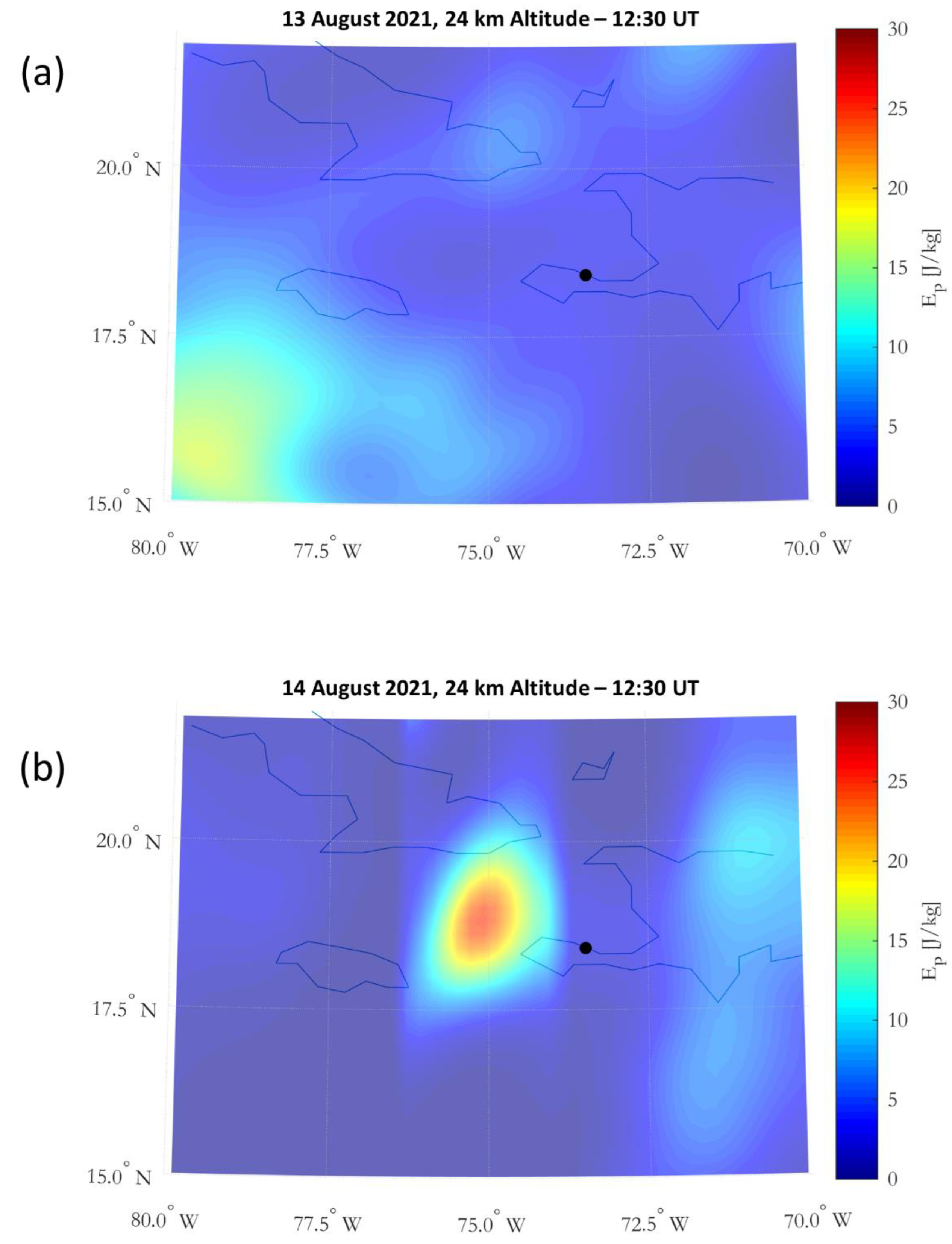
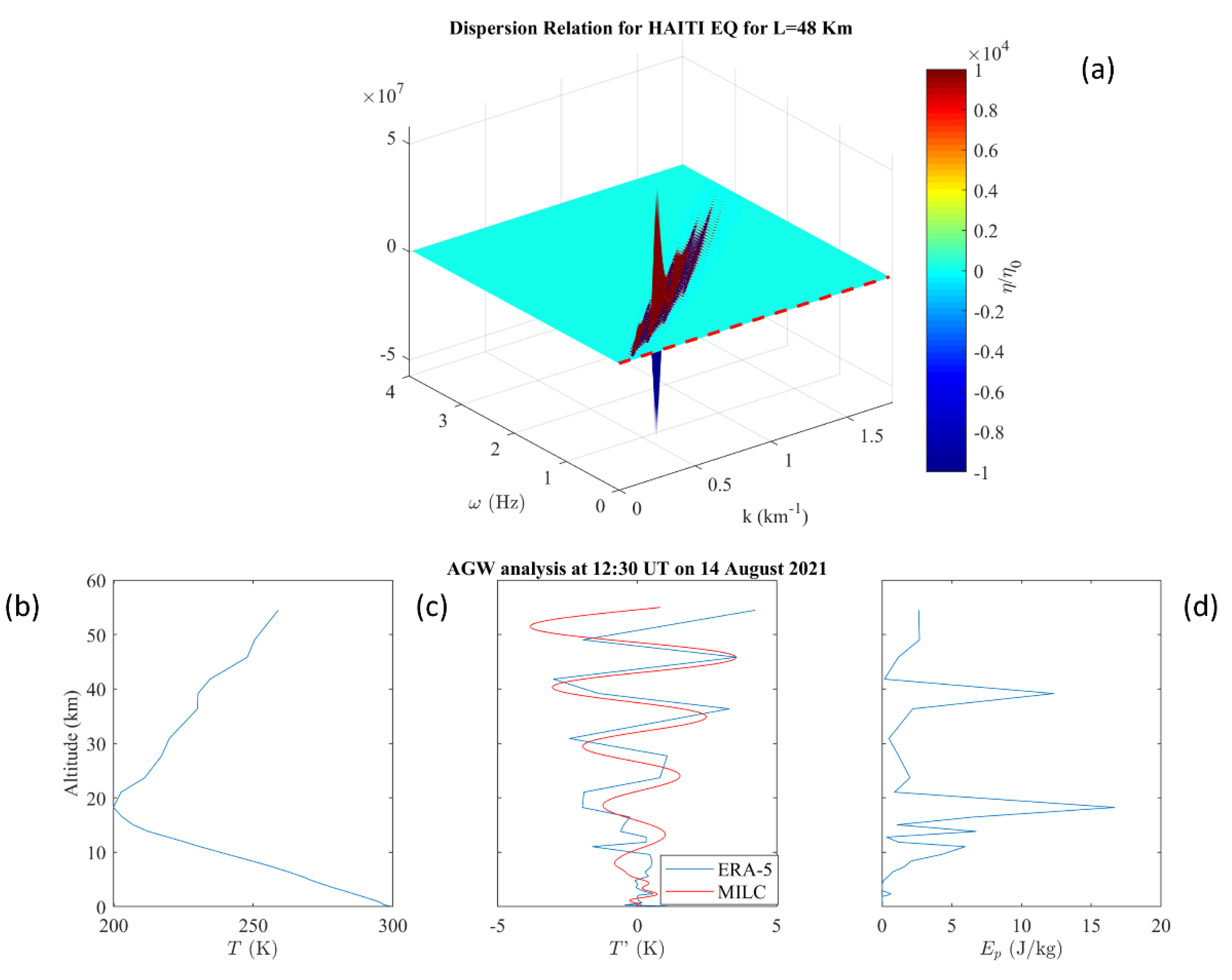
• An AGW in the atmosphere;
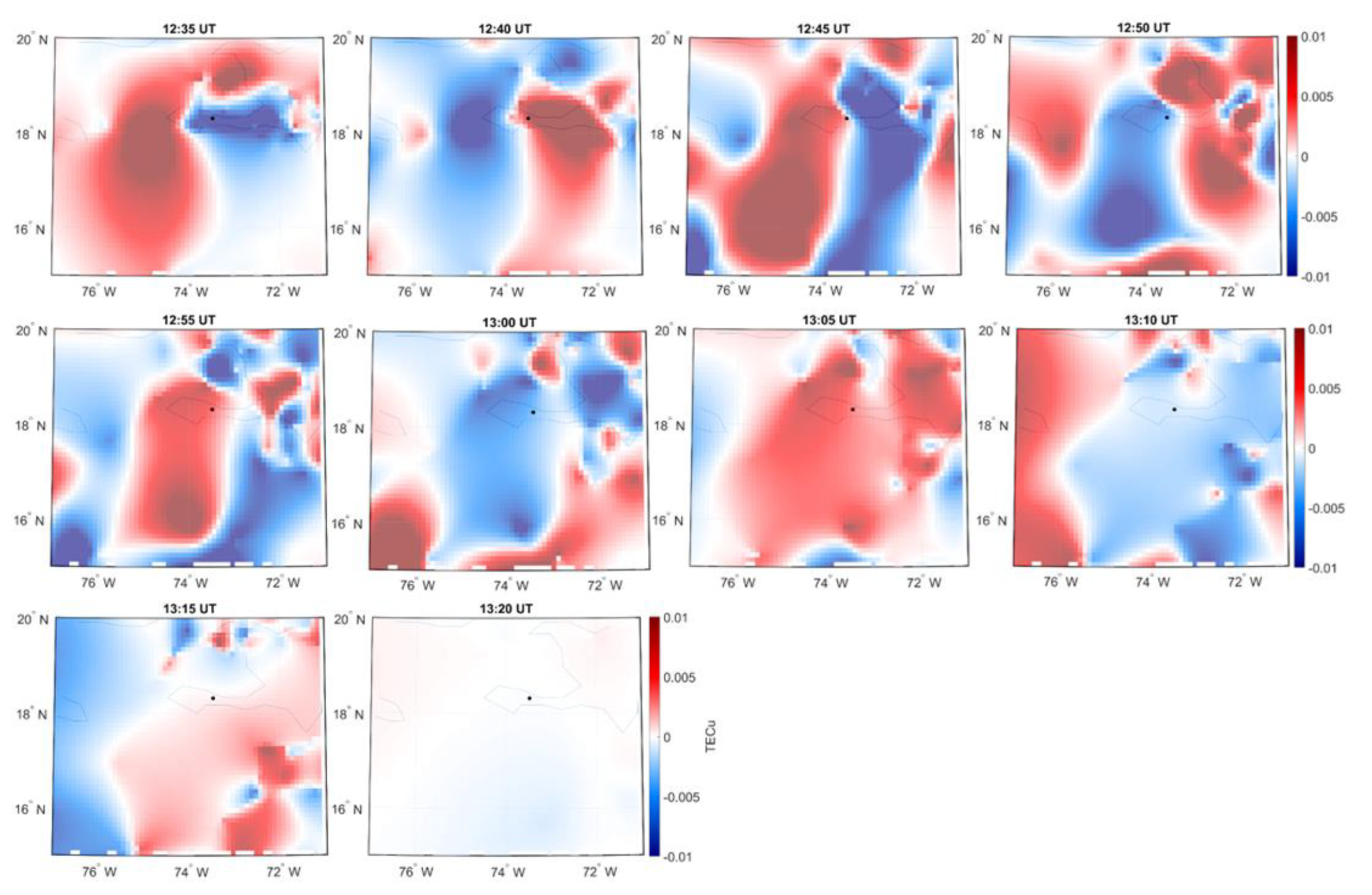
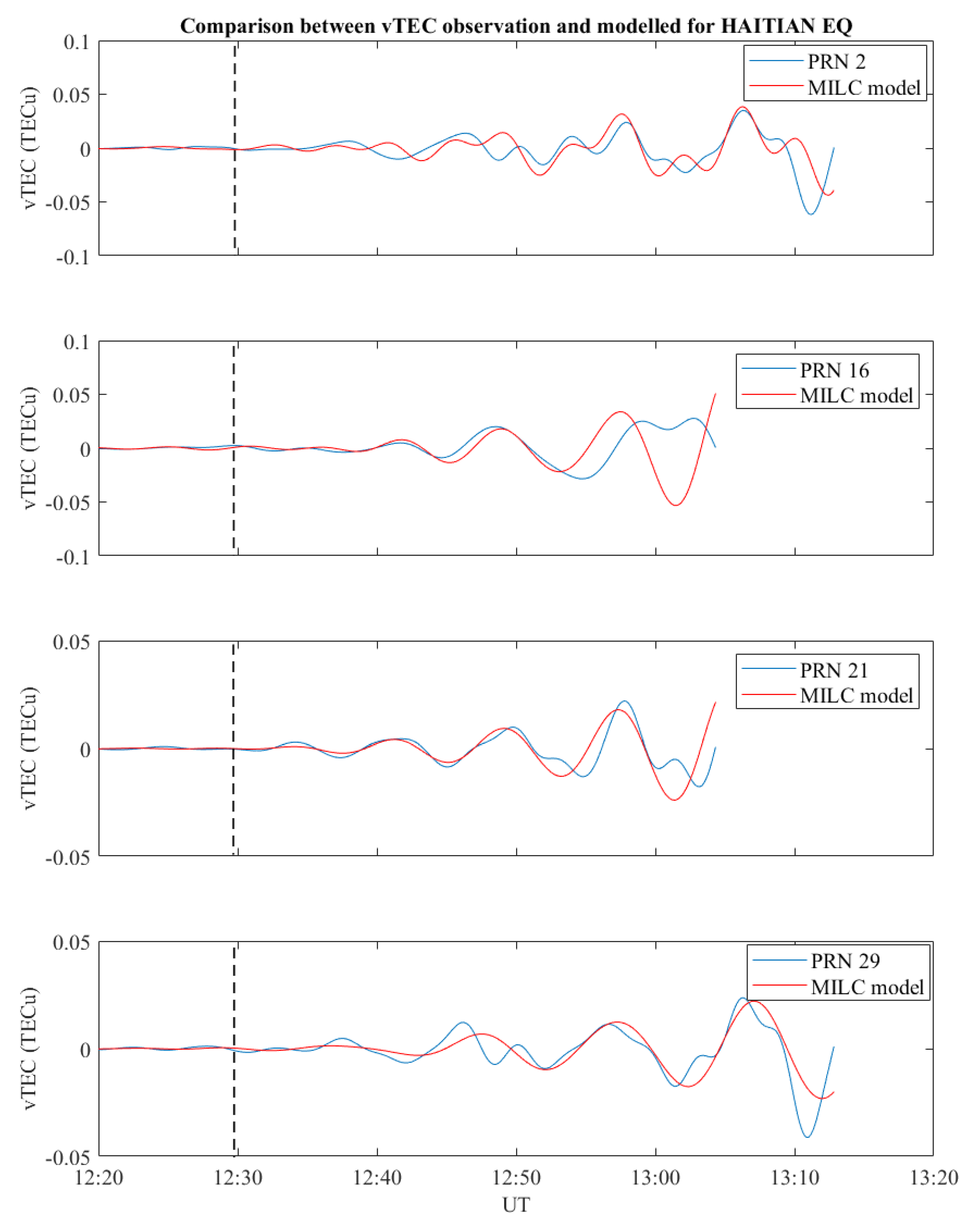
• A TID in the ionosphere;
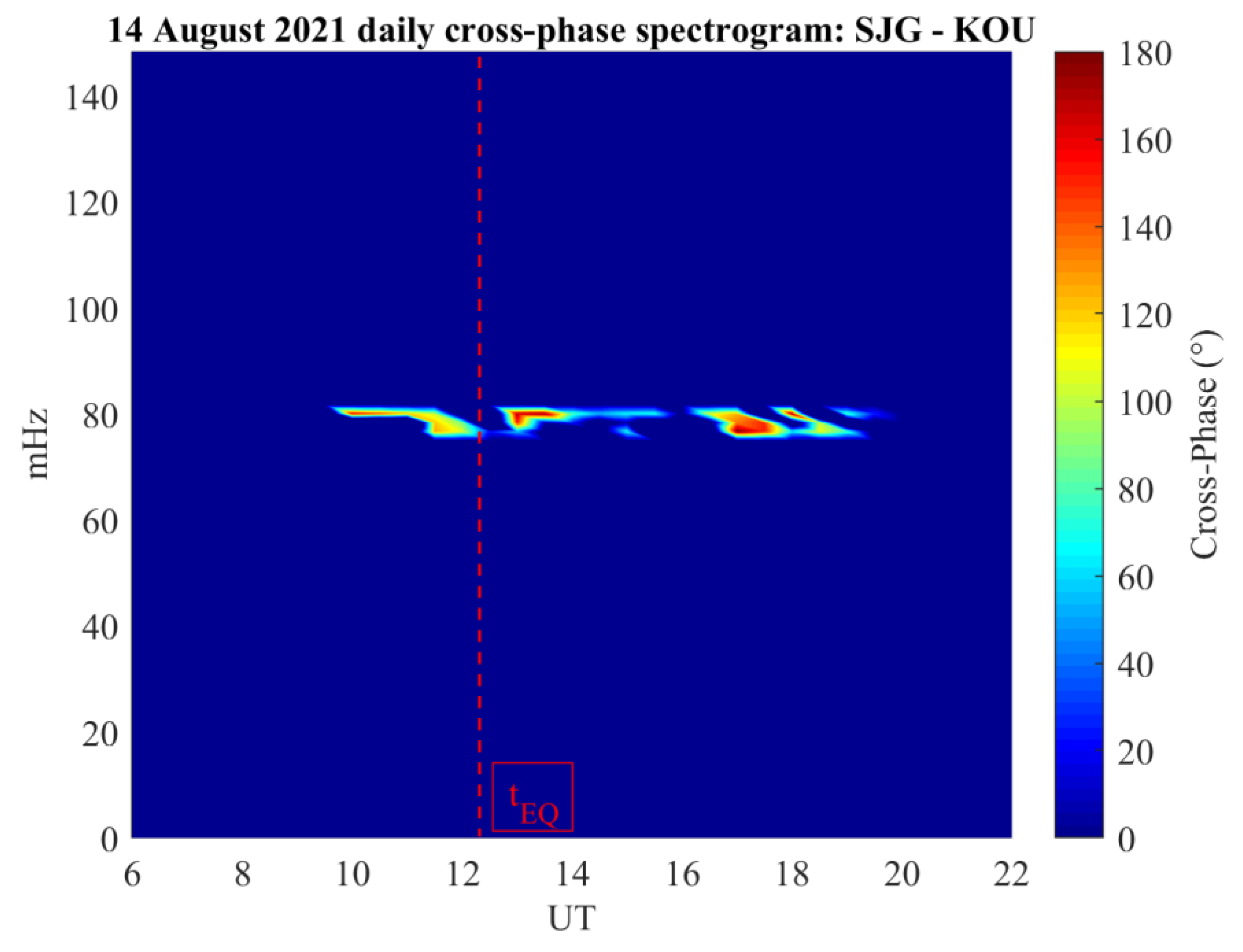
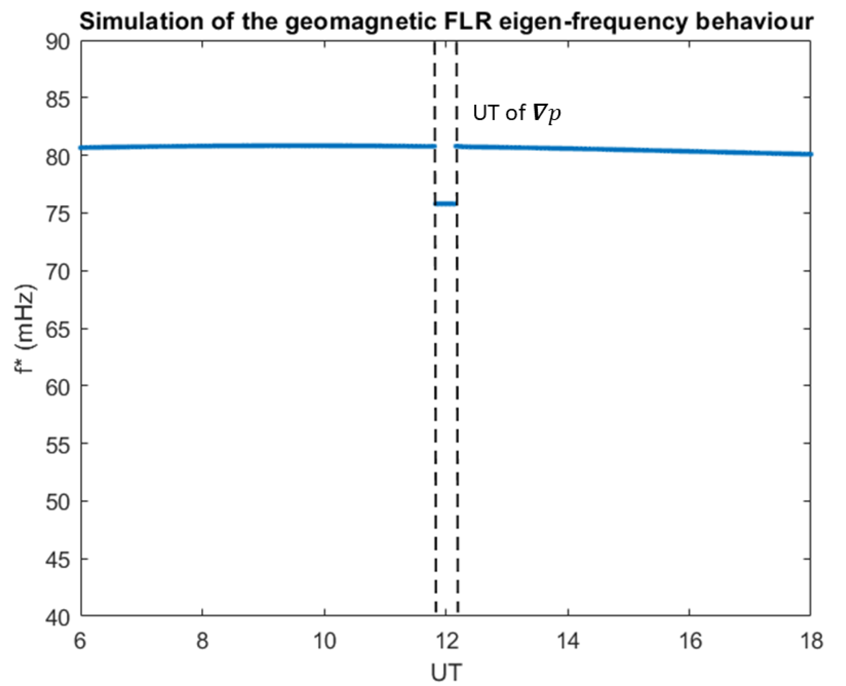
• A change in the magnetospheric FLR eigenfrequency.

On the other hand, after careful inspection of both space and atmospheric weather, and consequent exclusion of any competing confounder, we used the MILC model [14] to establish a causal relation between the detected signal at the different atmospheric layers and the EQ manifestation. As a result, we can reasonably conclude that the fault break generated an AGW able to reach the ionosphere and mechanically perturb its plasma density, leading to the magnetospheric FLR eigenfrequency variation.

References

1. Xiong, H. Recent advances in the research on seismo-electromagnetic emissions. Acta Seismol. Sin. 1992, 5, 407–412. [Google Scholar] [CrossRef]
2. Pulinets, S.; Boyarchuk, K. Ionospheric Precursors of Earthquakes; Springer Science & Business Media: Berlin, Germany, 2004. [Google Scholar]
3. Battiston, R.; Vitale, V. First evidence for correlations between electron fluxes measured by NOAA-POES satellites and large seismic events. Nucl. Phys. B-Proc. Suppl. 2013, 243, 249–257. [Google Scholar] [CrossRef]
4. Chakraborty, S.; Sasmal, S.; Basak, T.; Chakrabarti, S.K. Comparative study of charged particle precipitation from Van Allen radiation belts as observed by NOAA satellites during a land earthquake and an ocean earthquake. Adv. Space Res. 2019, 64, 719–732. [Google Scholar] [CrossRef]
5. Sgrigna, V.; Carota, L.; Conti, L.; Corsi, M.; Galper, A.; Koldashov, S.; Murashov, A.; Picozza, P.; Scrimaglio, R.; Stagni, L. Correlations between earthquakes and anomalous particle bursts from SAMPEX/PET satellite observations. J. Atmos. Sol.-Terr. Phys. 2005, 67, 1448–1462. [Google Scholar] [CrossRef]
6. Astafyeva, E.I.; Afraimovich, E.L. Long-distance traveling ionospheric disturbances caused by the great Sumatra-Andaman earthquake on 26 December. Earth Planets Space 2006, 58, 1025–1031. [Google Scholar] [CrossRef] [Green Version]
7. Calais, E.; Minster, J.B. GPS detection of ionospheric perturbations following the January 17, 1994, Northridge earthquake. Geophys. Res. Lett. 1995, 22, 1045–1048. [Google Scholar] [CrossRef]
8. Heki, K.; Otsuka, Y.; Choosakul, N.; Hemmakorn, N.; Komolmis, T.; Maruyama, T. Detection of ruptures of Andaman fault segments in the 2004 great Sumatra earthquake with coseismic ionospheric disturbances. J. Geophys. Res. Solid Earth 2006, 111. [Google Scholar] [CrossRef]
9. Liu, J.; Tsai, H.; Lin, C.; Kamogawa, M.; Chen, Y.; Lin, C.; Huang, B.; Yu, S.; Yeh, Y. Coseismic ionospheric disturbances triggered by the Chi-Chi earthquake. J. Geophys. Res. Space Phys. 2010, 115. [Google Scholar] [CrossRef]
10. Bonan, G.B. Land-atmosphere interactions for climate system models: Coupling biophysical, biogeochemical, and ecosystem dynamical processes. Remote Sens. Environ. 1995, 51, 57–73. [Google Scholar] [CrossRef]
11. Afraimovich, E.L.; Perevalova, N.P.; Plotnikov, A.; Uralov, A. The shock-acoustic waves generated by earthquakes. Ann. Geophys. 2001, 19, 395–409. [Google Scholar] [CrossRef]
12. Meng, X.; Vergados, P.; Komjathy, A.; Verkhoglyadova, O. Upper atmospheric responses to surface disturbances: An observational perspective. Radio Sci. 2019, 54, 1076–1098. [Google Scholar] [CrossRef] [Green Version]
13. Pokhotelov, O.; Parrot, M.; Fedorov, E.; Pilipenko, V.; Surkov, V.; Gladychev, V. Response of the ionosphere to natural and man-made acoustic sources. Ann. Geophys. 1995, 13, 1197–1210. [Google Scholar] [CrossRef]
14. Piersanti, M.; Materassi, M.; Battiston, R.; Carbone, V.; Cicone, A.; D’Angelo, G.; Diego, P.; Ubertini, P. Magnetospheric–ionospheric–lithospheric coupling model. 1: Observations during the 5 August 2018 Bayan Earthquake. Remote Sens. 2020, 12, 3299. [Google Scholar] [CrossRef]
15. Carbone, V.; Piersanti, M.; Materassi, M.; Battiston, R.; Lepreti, F.; Ubertini, P. A mathematical model of lithosphere–atmosphere coupling for seismic events. Sci. Rep. 2021, 11, 8682. [Google Scholar] [CrossRef] [PubMed]
16. Piersanti, M.; Burger, W.J.; Carbone, V.; Battiston, R.; Iuppa, R.; Ubertini, P. On the Geomagnetic Field Line Resonance Eigenfrequency Variations during Seismic Event. Remote Sens. 2021, 13, 2839. [Google Scholar] [CrossRef]
17. Yang, S.S.; Pan, C.-J.; Das, U. Investigating the Spatio-Temporal Distribution of Gravity Wave Potential Energy over the Equatorial Region Using the ERA5 Reanalysis Data. Atmosphere 2021, 12, 311. [Google Scholar] [CrossRef]
18. De la Torre, A.; Alexander, P.; Giraldez, A. The kinetic to potential energy ratio and spectral separability from high-resolution balloon soundings near the Andes Mountains. Geophys. Res. Lett. 1999, 26, 1413–1416. [Google Scholar] [CrossRef]
19. VanZandt, T. A model for gravity wave spectra observed by Doppler sounding systems. Radio Sci. 1985, 20, 1323–1330. [Google Scholar] [CrossRef] [Green Version]
20. Cai, X.; Yuan, T.; Liu, H.-L. Large-scale gravity wave perturbations in the mesopause region above Northern Hemisphere midlatitudes during autumnal equinox: A joint study by the USU Na lidar and Whole Atmosphere Community Climate Model. Ann. Geophys. 2017, 35, 181–188. [Google Scholar] [CrossRef] [Green Version]
21. Lu, X.; Chu, X.; Fong, W.; Chen, C.; Yu, Z.; Roberts, B.R.; McDonald, A.J. Vertical evolution of potential energy density and vertical wave number spectrum of Antarctic gravity waves from 35 to 105 km at McMurdo (77.8 S, 166.7 E). J. Geophys. Res. Atmos. 2015, 120, 2719–2737. [Google Scholar] [CrossRef]
22. Tsuda, T.; Nishida, M.; Rocken, C.; Ware, R.H. A global morphology of gravity wave activity in the stratosphere revealed by the GPS occultation data (GPS/MET). J. Geophys. Res. Atmos. 2000, 105, 7257–7273. [Google Scholar] [CrossRef]
23. Fritts, D.C.; Alexander, M.J. Gravity wave dynamics and effects in the middle atmosphere. Rev. Geophys. 2003, 41. [Google Scholar] [CrossRef] [Green Version]
24. Hennermann, K.; Berrisford, P. ERA5 Data Documentation; Copernicus Knowledge Base. 2017. Available online: https://confluence.ecmwf.int/display/CKB/ERA5%3A+data+documentation (accessed on 20 October 2022).
25. Hersbach, H.; Bell, B.; Berrisford, P.; Hirahara, S.; Horányi, A.; Muñoz-Sabater, J.; Nicolas, J.; Peubey, C.; Radu, R.; Schepers, D. The ERA5 global reanalysis, QJ Roy. Q. J. R. Meteorol. Soc. 2020, 146, 1999–2049. [Google Scholar] [CrossRef]
26. Ciraolo, L.; Azpilicueta, F.; Brunini, C.; Meza, A.; Radicella, S.M. Calibration errors on experimental slant total electron content (TEC) determined with GPS. J. Geod. 2007, 81, 111–120. [Google Scholar] [CrossRef]
27. Cesaroni, C.; Spogli, L.; Alfonsi, L.; De Franceschi, G.; Ciraolo, L.; Monico, J.F.G.; Scotto, C.; Romano, V.; Aquino, M.; Bougard, B. L-band scintillations and calibrated total electron content gradients over Brazil during the last solar maximum. J. Space Weather. Space Clim. 2015, 5, A36. [Google Scholar] [CrossRef] [Green Version]
28. Cicone, A.; Zhou, H. Numerical analysis for iterative filtering with new efficient implementations based on FFT. Numer. Math. 2021, 147, 1–28. [Google Scholar] [CrossRef]
29. Lin, L.; Wang, Y.; Zhou, H. Iterative filtering as an alternative algorithm for empirical mode decomposition. Adv. Adapt. Data Anal. 2009, 1, 543–560. [Google Scholar] [CrossRef]
30. Piersanti, M.; Alberti, T.; Bemporad, A.; Berrilli, F.; Bruno, R.; Capparelli, V.; Carbone, V.; Cesaroni, C.; Consolini, G.; Cristaldi, A. Comprehensive analysis of the geoeffective solar event of 21 June 2015: Effects on the magnetosphere, plasmasphere, and ionosphere systems. Sol. Phys. 2017, 292, 169. [Google Scholar] [CrossRef]
31. Cicone, A.; Pellegrino, E. Multivariate fast iterative filtering for the decomposition of nonstationary signals. IEEE Trans. Signal Process. 2022, 70, 1521–1531. [Google Scholar] [CrossRef]
32. Huang, N.E.; Shen, Z.; Long, S.R.; Wu, M.C.; Shih, H.H.; Zheng, Q.; Yen, N.C.; Tung, C.C.; Liu, H.H. The empirical mode decomposition and the Hilbert spectrum for nonlinear and non-stationary time series analysis. Proc. R. Soc. London. Ser. A Math. Phys. Eng. Sci. 1998, 454, 903–995. [Google Scholar] [CrossRef]
33. Wu, Z.; Huang, N.E. Ensemble empirical mode decomposition: A noise-assisted data analysis method. Adv. Adapt. Data Anal. 2009, 1, 1–41. [Google Scholar] [CrossRef]
34. Cicone, A. Iterative filtering as a direct method for the decomposition of nonstationary signals. Numer. Algorithms 2020, 85, 811–827. [Google Scholar] [CrossRef] [Green Version]
35. Flandrin, P. Time-Frequency/Time-Scale Analysis; Academic Press: San Diego, CA, USA, 1998. [Google Scholar]
36. Crowley, G.; Rodrigues, F. Characteristics of traveling ionospheric disturbances observed by the TIDDBIT sounder. Radio Sci. 2012, 47, 1–12. [Google Scholar] [CrossRef]
37. Menk, F.W.; Waters, C.L. Magnetoseismology: Ground-Based remote Sensing of Earth’s Magnetosphere; VCH: Weinheim, Germany, 2013; p. 251. ISBN 978-3-527-41027-9. [Google Scholar]
38. Okuwaki, R.; Fan, W. Oblique Convergence Causes Both Thrust and Strike-Slip Ruptures During the 2021 M 7.2 Haiti Earthquake. Geophys. Res. Lett. 2022, 49, e2021GL096373. [Google Scholar] [CrossRef]
39. Tsuda, T.; Murayama, Y.; Nakamura, T.; Vincent, R.; Manson, A.; Meek, C.; Wilson, R. Variations of the gravity wave characteristics with height, season and latitude revealed by comparative observations. J. Atmos. Terr. Phys. 1994, 56, 555–568. [Google Scholar] [CrossRef]
40. Waters, C.; Samson, J.; Donovan, E. Variation of plasmatrough density derived from magnetospheric field line resonances. J. Geophys. Res. Space Phys. 1996, 101, 24737–24745. [Google Scholar] [CrossRef]
41. Vellante, M.; Piersanti, M.; Pietropaolo, E. Comparison of equatorial plasma mass densities deduced from field line resonances observed at ground for dipole and IGRF models. J. Geophys. Res. Space Phys. 2014, 119, 2623–2633. [Google Scholar] [CrossRef]
42. Šindelářová, T.; Burešová, D.; Chum, J. Observations of acoustic-gravity waves in the ionosphere generated by severe tropospheric weather. Stud. Geophys. Et Geod. 2009, 53, 403–418. [Google Scholar] [CrossRef]
43. King, J.; Papitashvili, N. Solar wind spatial scales in and comparisons of hourly Wind and ACE plasma and magnetic field data. J. Geophys. Res. Space Phys. 2005, 110. [Google Scholar] [CrossRef]
Figure 1. USGS Community Internet Intensity Map (https://earthquake.usgs.gov/earthquakes/eventpage/us6000f65h/executive (accessed on 20 October 2022)). The black star highlights the earthquake epicenter.
Remotesensing 14 05340 g001
Figure 2. Co-seismic vertical profiles of: (a) temperature; (b) background temperature; (c) temperature deviation; (d) square of the Brunt–Väisälä frequency; and (e) potential energy at 12:30 UT on 14 August 2021. Red horizontal dashed lines represent the identified AGW peaks; from bottom to top, the green horizontal dashed lines identify the tropopause and the stratopause peaks, respectively.
Remotesensing 14 05340 g002
Figure 3. Horizontal distribution of the EP on (a) 13 August and (b) 14 August 2021 at 12:30 UT. The location of the earthquake epicenter is marked by the black dot.
Remotesensing 14 05340 g003
Figure 4. vTEC fluctuations characterized by a period between 7 and 12 min for all of the satellites in the field of view of all available GNSS receivers near the EQ epicenter (black dot) recorded every 5 min between 12:35 UT and 13:20 UT on 14 August 2021.
Remotesensing 14 05340 g004
Figure 5. The cross-phase dynamic spectrogram between two low-latitude ground stations near the earthquake epicenter.
Remotesensing 14 05340 g005
Figure 6. Weather report maps (https://www.wpc.ncep.noaa.gov/archives/web_pages/sfc/sfc_archive.php (accessed on 20 October 2022)) for the 14 August 2021 at 12:00 UT (panel a) and at 15:00 UT (panel b).
Remotesensing 14 05340 g006
Figure 7. Interplanetary space observations and geomagnetic response at low latitude on 14 August 2021. From top to bottom: Interplanetary Magnetic Field (IMF) intensity (a), Bx, IMF component (b), By, IMF component (c), Bz, IMF component (d), solar wind (SW) velocity (e), SW temperature (f), SW dynamic pressure (g), and SYM-H index (h) variations. The red dashed line marks the time of the earthquake occurrence.
Remotesensing 14 05340 g007
Figure 8. MILC model previsions for the AGW detected on occasion of the Haitian EQ on 14 August 2021. Panel (a) shows the dispersion relation of the AGW frequency and wavelength predicted by the MILC model, in which the red dashed line represents the parameter c0/2 h. Panel (b) shows the atmospheric temperature profile as observed by ERA-5; panel (c) shows the atmospheric temperature profile observed (blue line) vs. the predicted (red line); panel (d) shows the atmospheric potential energy density.
Remotesensing 14 05340 g008
Figure 9. Comparison between the vTEC fluctuations as observed (blue line) and predicted (red line) by the MILC model for four different GNSS satellites. The black vertical dashed line represents the time of the EQ occurrence.
Remotesensing 14 05340 g009
Figure 10. The FLR variation expected for the 14 August 2021 Haitian EQ as predicted by the MILC model. f* represents the modelled magnetospheric field line eigenfrequency.
Remotesensing 14 05340 g010