Article

Research on Self-Supervised Building Information Extraction with High-Resolution Remote Sensing Images for Photovoltaic Potential Evaluation

1
Aerospace Information Research Institute, Chinese Academy of Sciences, Beijing 100094, China
2
College of Resources and Environment (CRE), University of Chinese Academy of Sciences, Beijing 100049, China
3
School of Electronic, Electrical and Communication Engineering (EECE), University of Chinese Academy of Sciences, Beijing 100049, China
*
Author to whom correspondence should be addressed.
Remote Sens. 2022, 14(21), 5350; https://0-doi-org.brum.beds.ac.uk/10.3390/rs14215350
Submission received: 9 September 2022 / Revised: 18 October 2022 / Accepted: 20 October 2022 / Published: 25 October 2022
(This article belongs to the Special Issue Remote Sensing Based Building Extraction II)

Abstract

:
With the rapid development of the energy industry and the growth of the global energy demand in recent years, the development of the photovoltaic industry has become increasingly significant. However, the development of the PV industry is constrained by high land costs, and land in central cities and industrial areas is often very expensive and unsuitable for the installation of PV equipment in large areas. With this background knowledge, the key to evaluating the PV potential is by counting the rooftop information of buildings, and an ideal solution for extracting building rooftop information is from remote sensing satellite images using the deep learning method; however, the deep learning method often requires large-scale labeled samples, and the labeling of remote sensing images is often time-consuming and expensive. To reduce the burden of data labeling, models trained on large datasets can be used as pre-trained models (e.g., ImageNet) to provide prior knowledge for training. However, most of the existing pre-trained model parameters are not suitable for direct transfer to remote sensing tasks. In this paper, we design a pseudo-label-guided self-supervised learning (PGSSL) semantic segmentation network structure based on high-resolution remote sensing images to extract building information. The pseudo-label-guided learning method allows the feature results extracted by the pretext task to be more applicable to the target task and ultimately improves segmentation accuracy. Our proposed method achieves better results than current contrastive learning methods in most experiments and uses only about 20–50% of the labeled data to achieve comparable performance with random initialization. In addition, a more accurate statistical method for building density distribution is designed based on the semantic segmentation results. This method addresses the last step of the extraction results oriented to the PV potential assessment, and this paper is validated in Beijing, China, to demonstrate the effectiveness of the proposed method.

1. Introduction

With developments in society in recent years, global energy demand is gradually increasing every day and most consumption still relies on fossil fuels [1]. The use of fossil energy on a global scale has caused a series of problems such as melting glaciers and global warming. It is very important to change the energy structure and gradually replace current fossil energy with renewable energy [2]. It is also important to vigorously develop renewable energy for promoting green and low-carbon development and accelerating the construction of the ecological civilization. Among the many renewable energy sources, solar power generation is one of the most effective [3]. Solar power generation has the advantages of being inexhaustible, environmentally friendly, and not limited by geographical conditions [2]. The International Energy Agency predicts that solar photovoltaic (PV) power generation will become the main energy source and will account for 20–50% of global power generation by 2050 [4].
Solar power generation is mainly realized through crystalline silicon photovoltaic panels, which is also called photovoltaic power generation. Because it can be closely integrated with buildings and close to where electricity is used, it can reduce the transmission pressure on the power grid. However, in our investigation, we found that solar power generation depends on the intensity of sunlight and is greatly affected by extreme weather, which results in instability in both the power generation and supply time. This situation makes it very hard to transmit power to the grid. Therefore, it is necessary to evaluate the potential of PV system distribution and realize the unified dispatch of PV power and deploy PV equipment in areas with high electricity consumption to achieve the effect of “self-generation and self-consumption”. However, in areas with high power consumption, the deployment of PV systems is often accompanied by huge land costs. Distributed PV systems, which are necessary, are mainly installed on the roof of a building and are connected directly to a low-voltage distribution network. On the one hand, they have the advantages of proximity to the customer side, on-site consumption, and reduced transportation costs [5]. The roof of the building should have a strong load-bearing capacity and the generated electricity can be used directly in the building, reducing the costs of equipment and transportation dispatch. On the other hand, the building should have a long service life and PV equipment installed on the roof of a building can facilitate the recovery of installation costs; in addition, the roof of a building is the best platform to carry PV equipment [5]. Therefore, effective access to information about a building’s roof is the key to assessing the PV potential of buildings [6].
Conventional building information acquisition methods mainly rely on land surveys, which are difficult to acquire and have poor timeliness. Remote sensing satellite technology, which provides extensive access to ground information, has become a popular way to assess a building’s rooftop PV potential. In 2014, Flavio Borfecchia et al. used LiDAR technology and gis modeling tools to estimate urban roof levels under the three-dimensional view angle; this method was expensive but achieved significant evaluation results [7]. In 2016, Wong, MS et al. used remote sensing technology and geographic information system (GIS) technology to estimate the potential of photovoltaic power generation for the city of Hong Kong [8]. In 2018, Xiaoyang Song et al. conducted an assessment of building rooftop potential based on Google Images and global DEM data and calculated the annual rooftop photovoltaic power generation of buildings in Chaoyang District, Beijing, China. Specifically, they classified buildings into five types and further considered the tilt angle of PV panel installations for the PV potential assessment analysis, which had quite good inspirational and applied implications [9]. In 2019, Arti Tiwari et al. used orthophoto and LiDAR data with an object-oriented method to realize the evaluation of the solar energy yield in terms of solar irradiance in pixels in a specific period [10]. In 2020, Blazquez, J and Vittorio, M. used nighttime satellite imagery to assess the residential solar rooftop potential in Saudi Arabia [11]. In 2022, Huang, Xiaoxun et al. estimated the rooftop solar power generation potential in western Aichi Prefecture, Japan, based on the use of LiDAR data and AW3D technology [12]. It can be seen that a large number of researchers have chosen to use LiDAR data or high-resolution remote sensing data to extract building rooftop data. LiDAR data provides the possibility to obtain the building height and slope information for a fine-grained assessment of the PV potential. However, the cost of using LiDAR data is too high considering the large-scale statistical analysis. In contrast, using high-resolution remote sensing data is a cost-effective solution. However, when faced with a large amount of high-resolution remote sensing image data, it is time-consuming and laborious to use manual extraction of building information, and the value of remote sensing images is not fully exploited.
In recent years, the rapid development of deep learning algorithms has allowed for the extraction of spatial and spectral features at the same time so they are also widely used for the extraction of building data. Based on the adversarial neural network, Li Xiang et al. jointly trained a deep convolutional neural network (generator) and an adversarial discriminant network for the robust segmentation of building rooftops in remote sensing images and successfully solved the spatial inconsistency problem in classification [13]. Tian, Tian proposed an urban area target detection algorithm based on DCNNs, which still achieved good extraction results while maintaining the detection speed. Specifically, it used visual words based on DCNNs to extract feature information, thus realizing the extraction of data on urban areas without labeling samples; however, it was not accurate for specific buildings and its practical application accuracy was not good [14]. Zeng, Yifu et al. conducted experiments based on GF2 data and successfully realized the rapid extraction of building information. Specifically, their proposed BR-Net model used multi-task learning for segmentation and contour extraction to overcome limitations such as the unavailability of edge information [15]. Its effectiveness also illustrated the potential of multi-task learning. Based on the multi-task learning algorithm, Hui and Jian conducted building extraction experiments on the Massachusetts dataset and achieved good experimental results. The highlight of their article was the merging of distance representation into a multi-tasking framework as an auxiliary task, forcing the shared encoder to implicitly capture the features of the building structure [16]. However, the above methods were all supervised classification, and the effectiveness of the methods depended largely on the huge training samples. When the building information is extracted in a large area, due to the limitation of the samples, the extraction effect and accuracy of the model will be greatly affected. In recent years, many famous datasets have been proposed in remote sensing building information extraction, such as WHU [17], DOTA [18], Massachusetts [19], etc. These have largely advanced the rapid development of remote sensing information extraction technology. However, the applicability of the models obtained from the training of labeled data is often unsatisfactory due to the differences in spatial resolution, acquisition date, image location, and other elements.
Self-supervised learning methods, which have developed rapidly in recent years, have been evolving by automating the task of learning features to achieve the effective utilization of unlabeled samples. The latest comparative learning methods have achieved good results in some tasks and are very suitable for applications in building information extraction. Studying the application of self-supervised methods in remote sensing images is expected to provide a use for the huge amount of data that cannot be used in remote sensing, thus improving the generalization performance of deep learning models in the field of remote sensing information extraction. Among the many self-supervised learning methods, there are two main methods commonly used to train visual representations; one is a self-supervised learning method based on a reconstructed loss function and is often called the representational learning method [20,21], and the other is a self-supervised learning method that measures the contrastive loss of images and is often called the contrastive learning method. Among them, contrastive learning is the most state-of-the-art learning method in most cases [22,23,24,25]. Because of the good generalization of contrastive learning, it can also be developed more rapidly compared to representational learning methods. However, good representational learning tasks are more closely related to the target task so many breakthroughs in self-supervised learning have resulted from the discovery of representational learning tasks, although some researchers tend to use pretext tasks to extract features. In order to learn good representations, people have explored a variety of pretext tasks. A pretext task is meant to be a network task that provides pre-trained parameters, which can generally generate samples automatically without human intervention. Examples include colorization [26], contextual autoencoders [27], inpainting [21], spatial puzzles [28], and discriminative orientation [29]. Today, these self-supervised learning methods are collectively known as representational learning (as distinguished from contrast learning) methods and they can achieve very good results under specific tasks. With the development of self-supervised algorithms, the application of self-supervised learning in remote sensing image information extraction is also gradually emerging. Guo and Qing proposed a method for the automatic extraction of road centerlines from high-resolution remote sensing images based on a self-supervised learning framework. Good extraction results were achieved without the manual selection of training samples or optimization steps such as removing non-road areas [30]. Dong, Huihui et al. proposed a new self-supervised approach representing a time-based learning approach to predict remote sensing image change detection. The main idea of the algorithm was to convert two satellite images into a more consistent feature representation through the self-supervision mechanism without any additional computation of semantic supervision [31], thus reducing the propagation error of the final detection results. Li, Wenyuan et al. [32] designed three different pretext tasks to learn a multi-layer network structure simultaneously. The network was trained with a large amount of unlabeled data, fine-tuned with a small number of labeled segmentation datasets, and only used 10–50% of the labeled samples to achieve the original segmentation effect. In summary, it can be seen that self-supervised learning techniques have developed rapidly in recent years and have achieved excellent results in various tasks through the use of unlabeled data. Their success can be attributed to two aspects: the efficient use of unsupervised samples and the proper selection of the pretext task. Its essence involves the fusion of low-level features with high-level features of the image, and numerous experiments have shown that the fusion of these features can achieve even better segmentation results.
However, compared to general natural images (images taken by cameras, mobile cameras, surveillance cameras, and other ground equipment), satellite-derived remote sensing images have random views, more complex backgrounds, richer spectral features, and texture details. In addition, the above self-supervised methods designed for natural images (photos taken by cameras, mobile cameras, surveillance cameras, and other ground equipment) do not fully consider the characteristics of remote sensing images. This migration of features obtained through pretext task learning of remote sensing targets may not have the expected effect. In addition, the evaluation of building rooftop PV power potential involves a large amount of building information extraction, and traditional deep learning methods require a large number of building samples to ensure that the model can have good generalization ability. The extraction structures between deep learning tasks can be used mutually so that the self-supervised model can use pre-training to obtain a priori information and its extraction effect will be better than random initialization. However, existing self-supervised learning methods have a gap between the pretext task and the target task, which is usually more generalized for the pretext task and more aggregated for the features required by the target task; by using practical self-supervised methods for pre-training, it is often difficult to obtain good experimental results [33].
To address the above issues, we propose a pseudo-label-guided self-supervised learning method (called the PGSSL method), which utilizes pseudo-label learning to guide the pretext tasks. In detail, feature layer sharing is used to achieve the mutual utilization of the feature extraction part for the task interaction between different tasks and the utilization of unlabeled data. The effectiveness of our proposed structure is demonstrated by comparison experiments with different sample proportions and ablation experiments with different structures. The main contributions of this paper are as follows:
  • In this paper, a self-supervised learning framework for semantic segmentation is proposed considering the characteristics of remote sensing images, and it is demonstrated that a large number of unlabeled remote sensing images can be effectively used to train the network. For the self-supervised learning task, this paper designs a self-supervised structural method for multi-task learning called the PGSSL method. It improves the performance of the semantic segmentation task by guiding feature extraction with a pseudo-labeling task.
  • The proposed method is validated on a public dataset (EA Dataset) and an independently constructed Beijing dataset (BJ Dataset), comparing the performance of algorithms under different sample conditions and verifying the good performance of the self-supervised learning method with a limited sample size. Finally, our method achieves better results than the ImageNet pre-training in the experiments.
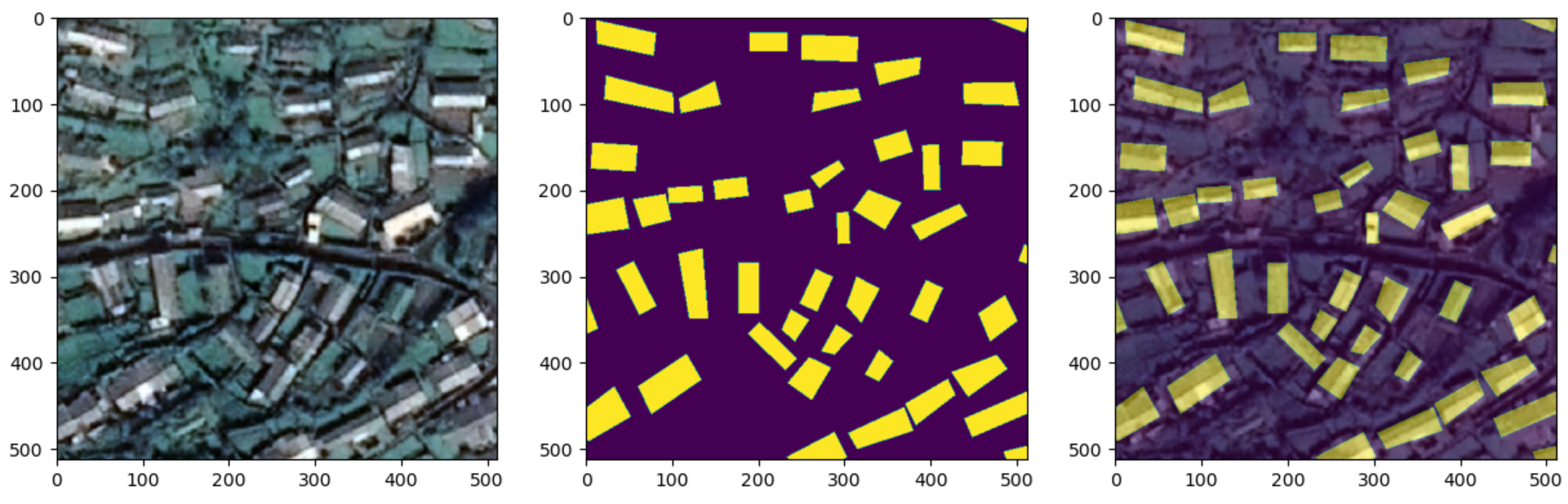
  • In this paper, we further analyze the distribution of buildings based on the semantic segmentation of the buildings to obtain a more accurate picture of the suitability of building rooftops for the installation of PV equipment.
The full text is organized as follows. Section 2 introduces the self-supervised learning strategy based on pseudo-label guidance and the method of using the semantic segmentation results for the PV potential assessment. Among them, the self-supervised approach is introduced and includes three modules: a pseudo-label learning module, an image inpainting module, and a comparative learning module. Section 3 presents the datasets used for the experiments and the formulas used for the accuracy assessment. The dataset section presents detailed information on the Beijing dataset and the public dataset. It includes the study area, data sources, and the method of obtaining unlabeled data. Section 4 presents three comparative experiments of the proposed method in this paper, including the overall algorithm effect comparison, the sample proportion experiment, and the ablation experiment. Section 5 summarizes and discusses the paper, discusses and analyzes the phenomena that were observed during the experiments, and provides an outlook on some directions that can be pursued.

2. Methods

In this paper, we design a multi-task learning model based on pseudo-label learning. This paper designs contrastive learning and image inpainting tasks to extract features from unlabeled data, where the image restoration task helps the network to learn low-level features and the contrastive learning task enables the network to learn high-level image features. In addition, this paper designs pseudo-label learning to ensure that the learned features can be adapted to the final target task extraction. The relevant code can be found at https://github.com/Chendeyue/pytorch-ssl-building_extract, accessed on 7 August 2022.
The overall structure of the work is shown in Figure 1. It can be seen that the main body consists of three parts: pseudo-label training, image inpainting, and contrastive learning, which share a common feature extraction layer. In the two parts of the pseudo-label training and image restoration, the UNet network is chosen as the structure of the intermediate implementation, and the skip-connection structure of the UNet framework is used to achieve the full utilization of the features. In the final classification layer, pseudo-label learning classifies the targets into two classes corresponding to the probabilities of buildings and non-buildings, whereas the image inpainting task outputs three classes corresponding to the three bands of the newly generated images. The decoding parts of both are independently constructed networks that do not share network parameters. The contrastive learning task part mainly adopts the idea proposed in BYOL to design a twin network structure with a momentum update. For a set of input data-enhanced images, two feature vectors are generated after passing through the twin network separately. The two vectors generated by the twin network are cross-compared separately and a similarity loss function is constructed, as shown in Figure 1, to achieve comparative learning of the network features. Finally, the three unsupervised task loss functions are combined to form a multi-task learning structure to accomplish a self-supervised learning task. Its loss function is shown in Equation (1).
L f i n a l = λ 1 L p s e u d o + λ 2 L c o n t r a s t + λ 3 L i n p a i n t i n g
where λ is a hyperparameter used to balance the magnitude difference between three types of loss and λ 1 = λ 2 = λ 3 = 1 3 . L p s e u d o , L c o n t r a s t , and L i n p a i n t i n g denote the loss of several parts; details can be found in Equations (4), (6), and (8). Since the three loss functions have a similar status and approximate value range, we take the mean value to balance the three tasks.

2.1. Weighted Training on Pseudo-Labeled Data

Pseudo-label learning is a semi-supervised learning method that has emerged in recent years. The core idea is to build a model using existing knowledge and use it to predict unlabeled samples to obtain the pseudo label. The pseudo label is trained using prior knowledge to learn information from unlabeled data. Finally, the results with relatively high confidence in prediction are used as labels to ensure the accuracy of the labels.
In this paper, the pre-training trained network is called the teacher network and the pseudo-label learning channel to be trained is called the student network. These networks are structurally similar but are independent network models and their parameters are not shared. Both the teacher network and the student network have unlabeled augmented images as input, where the teacher network is the trained model and the student network relies on the labeled training generated by the teacher network. In addition, the parameters of the teacher network are not updated when training the student network. The training process is as follows: first, we train a teacher network using the enhanced labeled dataset, then, the teacher network predicts the input image as the pseudo-label, named q j , and finally, the result with high confidence in q j is compared with the result q ^ j of our student network to be trained. This completes the learning of the pseudo-label part, which is done in parallel with the other two tasks, and with the guidance of pseudo-label learning, the extracted feature layer parameters can be more suitable for migration to the target task. The final loss function is shown in Equation (4):
H ( q ^ j , q j ) = b = 1 C q ^ j ( b ) log q j ( b )
L x = 1 N j = 1 N ( L ( m a x ( q j ) τ ) * H ( q ^ j , q j )
L p s e u d o = 1 2 ( L x 1 + L x 2 )
Here, q j = P t ( y | x j ) and q ^ j = a r g m a x ( P s ( y | x j ) ) , which denote the prediction results of the output of the teacher network that has been fitted and the student network that is being trained, respectively, where τ is the threshold hyperparameter used to filter unsupervised samples. We keep the corresponding pseudo labels only when the maximum predicted probability is higher than the threshold, which is usually taken as 0.5. C is the number of categories, N is the number of samples, and H is the entropy value function. L ( m a x ( q j ) τ ) represents the probability that the prediction threshold exceeds a certain value, usually equal to 1 or 0. The loss function, called L x , is calculated as the result of inputting image x into the teacher network and the student network, respectively, whereas L x 1 and L x 2 denote the loss obtained by two different data enhancement methods.

2.2. Contrastive Learning Task

The contrastive learning task achieves the convergence of the network by comparing the similarity of images. The operation is as follows: first, the images are transformed with data augmentation and then, the similarity between the transformed image results is compared to construct a loss function. Theoretically, the higher the similarity of the features in an image, the smaller the loss. This allows all similar objects to be located in adjacent positions in the feature space, whereas dissimilar objects are located in non-adjacent regions.
In recent years, researchers have proposed effective comparative learning methods such as SimCLR [24], MOCO [22], MOCOv2 [34], BYOL [25], etc. In most comparative methods, we must compare each sample to many other negative samples. However, it makes training very unstable and increases the systematic bias of the dataset. The proposal of the BYOL method [25] provides a proper solution to this problem. The BYOL method does not rely on negative samples but only uses similar sample representation types to construct a loss function. The final loss function is shown in Equation (6):
C o s i n e S i m i l a r i t y ( p , z ) = i = 1 B p i z i i = 1 B p i j = 1 B z j
L c o n t r a s t = C o s i n e S i m i l a r i t y ( p 1 , z 2 ) + C o s i n e S i m i l a r i t y ( p 2 , z 1 )
Here, L c o n t r a s t represents the contrastive loss function and B is the dimension of the vector. CosineSimilarity represents the cosine similarity between two vectors. The outputs of pi and zi are shown in Figure 1, representing the outputs of the online network and target network, respectively, whereas p1 and p2 represent the global feature vectors inputted by two different data augmentation methods and p1 and z2 and p2 and z1. This alternate combination method for the similarity verification brings greater flexibility to the model, and the main feature extraction network used in the comparative learning process is shared with the other two tasks to ensure that the extracted features are closer to the direction of the target task.

2.3. Inpainting Task

The image inpainting pretext task itself is used to restore the missing parts of an image based on the existing information in the image. However, in the process of image inpainting, because the conventional loss function is generally adjusted globally for the image, this will make the inpainting task only supplement the image information that is similar to the global image and ignore the use of local texture information. To solve this problem, this paper adopts SSIM [35] (structural similarity index) to construct the inpainting loss function, but the global variance of the image fluctuates greatly in the actual operation so the SSIM value is only calculated in one window and then the mean value is taken globally. The specific form is shown in Equation (8):
S S I M ( x , y ) = ( 2 μ x μ y + C 1 ) ( 2 σ x y + C 2 ) ( μ x 2 + μ y 2 + C 1 ) ( σ x 2 + σ y 2 + C 2 )
L i n p a i n t i n g = M S S I M ( x , y ) = 1 N j = 1 N S S I M ( x j , y j )
Here, μ x and μ y represent the mean values of the input image and the output image; σ x y , σ x , and σ y represent the covariance and variance of the two images; and C1 and C2 are constants. x and y represent the images before and after restoration, respectively, and MSSIM is a better final loss function for the image inpainting task.

2.4. Analysis of Photovoltaic Potential Area Based on Building Semantic Segmentation

The rooftop area of a building is the most important influencing factor for the PV potential assessment, and accurate rooftop extraction results are the basis for the PV potential analysis. However, in practice, the supporting facilities for PV equipment installation, as well as its scale, can also be a constraint to the building’s potential. Even if an area has a large building area but the rooftop area of each building is small and the buildings are scattered, the high cost of the supporting facilities would mean that the buildings in the area would not be considered a distributed PV installation area. The semantic segmentation results can only evaluate the installed area of the building and not the distribution. As shown in Figure 2, for the semantic segmentation of the connected domain analysis results, where there is a relatively large degree of separation between buildings, such as in region A and region C, the suitability of PV installation on buildings can be better assessed; however, in the case of the buildings in region B, the actual installation for the patches of private houses is more complex, but it may be identified as an area with better PV potential due to its larger area.
Therefore, in practical applications, when using the semantic segmentation results to evaluate the distribution of buildings, it is necessary to further segment the connected buildings and remove some noise blocks. In this paper, the morphological opening operation is used to exclude some noise spots from the extraction results and the confidence characteristics of the deep learning prediction are used to separate the connected building patches. The specific operation is shown in Figure 3. First, starting from the original image, by controlling the confidence level of the prediction of the original image, the conventional confidence level results for building area extraction are more accurate and the high confidence level results for the separation degree between buildings are obtained.
Then, we perform a morphological opening operation on the conventional results to obtain the building distribution results with the noise patches removed, directly extract the center point of the patch for the high-confidence results, and perform the superposition analysis of the extracted center point results and the opening operation results. After removing the center point of a small part of the noise, a relatively accurate building distribution is obtained.

3. Dataset and Evaluation Metrics

3.1. Dataset

In order to fully illustrate the generalization performance of the proposed method in experiments in various regions, this paper independently produced urban and rural datasets in Beijing for the experiments called the BJ Dataset (Beijing Buildings Segmentation Dataset). The remote sensing data used in the experiments include Google data and SV-1 data. Located in Haidian District, Xiangshan District, and Yajishan District of Pinggu District, Beijing, the average resolution was about 1 m. The locations of the training areas and the basic conditions of the images are shown in Figure 4A–D. After using ArcGIS to label all the buildings in the target area, the training area images were cut into a 384 × 384 size and divided into the training set and test set, according to a ratio of 4:1, and finally, 797 training sets and 202 validation sets were obtained.
This paper also collected some regional data in Beijing and Tianjin for experimental testing. The data used were all Google receipts and their locations and images are shown in Figure 4E,F. After the images were manually annotated, they were also cropped to a 384 × 384 size, resulting in 16 slice results in the test area in Beijing and 34 slice results in the test area in Tianjin. The schematic diagram of one of the slice results in the Tianjin area used for verification is shown in Figure 5.
The construction of the dataset also included the acquisition of unlabeled samples because in a whole remote sensing image, if the specific features of buildings are very small when using all the tiles of the region for training, the construction of unsupervised samples of buildings needs to further eliminate the tile images that do not contain buildings. Therefore, this paper first collected the Beijing area 1 m-resolution Google images and cropped them to 384 × 384-size tiles to obtain a total of 21,417 unlabeled building images. Subsequently, a building extraction model was trained to predict the collected image tiles using the above-labeled samples and the tiles without buildings in the prediction results were excluded. Finally, we excluded a few images with relatively poor quality by manual inspection.
In addition, in order to fully verify the actual effect of this model, a public dataset was used for the experiments, which came from Wuhan University [17] (http://study.rsgis.whu.edu.cn/pages/download/building_dataset.html, building Dataset, accessed on 9 September 2022) and is referred to here as the EA (East Asia) dataset. The EA dataset consisted of 6 adjacent satellite images covering 860 square kilometers of East Asia with a ground resolution of 0.45 m. The architectural styles were quite different, and the generalization ability of the deep learning methods on the different data sources was fully evaluated and developed. The vector building map was also drawn manually by ArcGIS software and contained 34,085 buildings. The entire image was seamlessly cropped into 17,388 blocks of 512 × 512 as a result. Excluding the dicing results that did not contain buildings, the remaining training set contained 25,749 buildings (3135 slice results) and the test set contained 8358 buildings (903 slice results). For the convenience of the experimental comparison, the training set was randomly divided into 2508 training sets and 627 validation sets according to a ratio of 4:1, and the result of one slice is shown in Figure 6.
Among them, the unlabeled data used for the self-supervised training for the independently produced the Beijing area sample set were from Google data for the whole of the Beijing area. For the EA dataset, the unlabeled data were from the results obtained by merging all data. A brief introduction to the two datasets is shown in Table 1.

3.2. Evaluation

In this article, we used the F1-score to evaluate the results. In order to evaluate the effectiveness of the image pixel-level prediction task, we compared the prediction results with the corresponding ground truth and divided each pixel into true positive (TP), false positive (FP), false negative (FN), and true negative (TN). The evaluation metrics used to measure the effectiveness of our method were calculated based on these four indicators. The F1 score is the reconciled average value of the recall rate and accuracy rate according to specific formulas, as shown in Equations (9)–(12):
P r e c i s i o n = T P T P + F P
R e c a l l = T P T P + F N
I O U = T P T P + F P + F N
F 1 _ s c o r e = 2 × P r e c i s i o n × R e c a l l P r e c i s i o n + R e c a l l
where TP denotes true positive, FP denotes false positive, and FN denotes false negative. These indicators were calculated using each tiled pixel-based confusion matrix or cumulative confusion matrix and are explained in the following section.

4. Results and Discussion

4.1. Experimental Setup

To validate the effectiveness of the proposed method for building information extraction, we conducted experiments on two datasets and compared our model with state-of-the-art methods. For semantic segmentation methods with conventional supervised learning, this paper compared three semantic segmentation frameworks, Unet, PSPNet, and Deeplabv3+. Secondly, based on the Unet structure, we validated the basic experimental results of several popular comparative learning methods and the proposed PGSSL method in this paper on two datasets, as well as the extraction effects under different proportional sample inputs. Finally, this paper conducted ablation experiments on the PGSSL structure under two datasets to verify the effectiveness of each link design. The parameters used for each part of the network are shown in Table 2.
For the selection of the underlying network structure and data augmentation, to ensure the consistency of the experimental process, the experiments in this paper all used ResNet34 as the basic network feature architecture. Firstly, a 7 × 7 convolutional kernel with pooling was used to expand the feature dimension to 64 and the image size was downsampled to 1/4 of the original size. Subsequently, after several convolutional poolings, the final feature map size became 1/32 of the original size and the feature channel was expanded to 512 dimensions. To make full use of the sample features, we randomly augmented the data before training and the data augmentation methods we used included random color transformation, random flip, random rotation, random crop, and resampling in five steps, the specific parameters of which are shown in Table 2 Data Augmentation. Data augmentation was not applied in any of the data testing.
The network training parameters of this paper included two parts, the pretext task network training and the semantic segmentation network training. For the training part of the pretext task network, the input image batch was 8, the total number of iterations was 80,000, the learning rate was set to 3 × 10 4 , and after every 10,000 iterations, it was reduced to 95% of the original, and it took about 11 hours to complete the pretext task network. For the semantic segmentation part of the training, the loss function used the cross-entropy function, the input image batch was also set to 8, and the initial learning rate was set to 0.005. We calculated the accuracy of the validation set every 150 iterations and saved the model with the highest accuracy and stopped training after 80,000 iterations.

4.2. Comparison of Different Methods

Following the above methods and parameter settings, this paper first conducted experiments using complete training samples on two datasets. For conventional semantic segmentation methods, such as PSPnet [36], Deeplabv3+ [37], and UNet [38], the labeled samples were directly used for training. We kept the best-trained model in the validation set obtained during the training process and finally calculated the accuracy obtained by testing on the test set, as shown in Table 3. The main experiments were divided into two main parts, basic framework training and self-supervised learning training. All experiments in this paper were repeated three times and the best results were used to explore the upper limit of the model approach. In the supervised learning task, the basic network modules were initialized with the ImageNet parameters, except for the special annotation of UNet(Random). After comparison, the Unet structure maintained the best test results among the three traditional semantic segmentation networks.
For the self-supervised methods, such as SimCLR [24], BYOL [25], and PGSSL, in this paper, we first trained the network in unlabeled samples, then trained the network under the self-supervised framework until the loss was minimized, and finally, transferred the parameters of the feature extraction layer to the UNet network framework. In the subsequent training, only the parameters of this part were fine-tuned and the learning rate was set to 0.1 of the regular learning rate. After collecting the best models on the ensemble, the accuracy obtained by testing on the test set was used as the final prediction accuracy. The training of PGSSL consisted of three steps due to pseudo-label learning. First, it provided a basic model for regular training for pseudo-label training and then self-supervised learning training was performed on top of that. This process generated pseudo-label channel prediction results with prediction accuracies as shown in Table 3 PGSSL, and finally, the basic feature structure generated by the above model was used for initial learning and training to obtain the final model test results, as shown in Table 3 PGSSL * . For the BJ Dataset, this paper mainly tested the final results of the model on areas E and F in Figure 4. To illustrate the generalization of the model, the F1-score of the test for the E area was 83.3% and the F1-score for the F area was 77.0%. The accuracy comparison of the subsequent methods was based on the test results of the F area. The overall differences between the methods are shown in Table 3.
From the comparison in Table 3, it can be seen that the underlying results showed that the Unet structure had the highest accuracy among several semantic segmentation frameworks on both building datasets. Second, initializing the network structure using ImageNet significantly improved the model testing accuracy relative to random initialization, with a 3.6% increase in the F1-score in the BJ dataset and a 6.5% increase in the F1-score in the public data. Finally, self-supervised learning significantly improved the model results, which was even more significant in the BJ dataset, where the F1-scores of the commonly used SimCLR and BYOL methods improved the accuracy by 2.6–2.9% over the original ImageNet, and the final PGSSL method improved it by 5%. The segmentation effects in the two datasets are shown in Figure 3. The effects on the images are shown in Figure 7, where Figure 7a–e show the prediction results for the BJ dataset and Figure 7f–j show the prediction results for the EA dataset.
However, it can also be seen in Table 3 that the improvement effect of the relevant self-supervised methods on the public dataset was much lower than that on the BJ Dataset. After analysis, we believe that this was mainly related to the number of labeled samples and the quality of unlabeled data in the self-supervision. Relatively speaking, the public dataset was relatively rich in labeled data when the learning no longer relied on the prior knowledge provided by the pre-training network and only needed to provide the basic pre-training structure to achieve better segmentation results. In addition, the public data did not additionally collect local unlabeled data. The images used in the self-supervised learning process were from the images needed for the subsequent semantic segmentation and the additional prior knowledge that was provided was relatively limited.

4.3. Experiments with Different Sample Ratios

In order to illustrate the effectiveness of the self-supervised method, this paper conducted experiments on the optimization effect of self-supervised learning with a small number of samples. We randomly selected a certain percentage of samples from the training part of the two datasets for the experiments, including 1%, 5%, 10%, 20%, 50%, 80%, and 100%. In this paper, we compared the experimental results of two datasets with different methods at different sample proportions. Among all the methods, the PSPNet, Deeplabv3+, and UNet networks were trained using ImageNet pre-training network initialization, whereas the other self-supervised learning methods were trained on the corresponding structures and migrated to Unet structures. In this paper, we compared our approach with two state-of-the-art self-supervised representation learning methods following the experimental setup in Section 4.1, firstly for the BJ dataset, where PGSSL represented the model output in the pseudo-label channel and PGSSL* represented the further pre-training results; all the experimental results are shown in Table 4.
In the BJ dataset experiments, the accuracy showed a significant upward trend with the increase in the sample proportion. Secondly, when the sample proportion was small, the basic UNet semantic segmentation network structure showed better stability at this time. At 1% of the samples, only about eight images were randomly selected from the original training data center for training and achieved a 63.6% segmentation accuracy, which was second only to the results initialized with SimCLR. The overall change can be seen in Figure 8a. In the EA dataset experiments, the method proposed in our paper always maintained the leading accuracy. However, as the sample size increased, the improvement in accuracy was no longer significant. In the BJ dataset, the training sample size did not reach the limit of potential for this method. As predicted by the current results, it is worth exploring the effect of further supplemental samples to experiment with self-supervised learning. The changing trend is shown in Figure 8b.
Comparing the UNet network structure with the final segmentation results of PGSSL in this paper, it can be seen that when the sample size was greater than 10%, PGSSL outperformed the former and other self-supervised learning methods. However, when the sample size was very small (the proportion was less than 10%), the results showed a significant decrease. We think this is because pseudo-label learning was used in the structural design to guide the process of self-supervised learning, and when the labeled samples were too small, the actual generalization ability of the model used for guidance was poor, thus providing incorrect guidance to the whole model. Furthermore, it can be seen that the SimCLR self-supervised learning method surpassed the results using all samples by using only 50% of the samples. This was a special case among all the experiments in this paper, but it also shows that the self-supervised learning method has a high upper limit and the prior knowledge from pre-training provides better possibilities for the model.
However, there are some differences between the experiments on the EA dataset and the experimental results of the previous paper. As shown in Table 5, the self-supervised learning method performed better when the sample size was less than 20%, especially when the sample size was 1%; the method proposed in this paper resulted in a 3.2% accuracy optimization, and the other self-supervised learning methods and the output of the pseudo-label channel also improved in this process. After the sample size was increased, it can be seen that the accuracy of the self-supervised learning method was almost the same as the results of conventional ImageNet pre-training. This paper suggests that this reflects a boundary effect that network pre-training can have. When the sample size reaches a certain level, the effect of prior knowledge provided by the pre-training of self-supervised learning decreases.

4.4. Ablation Experiment

Finally, in order to verify the effectiveness of the proposed structure, this paper also conducted ablation experiments on several selected proxy tasks to compare the effects of these different proxy tasks on building information extraction. Considering that the method proposed in this paper requires a pre-training structure to provide prior knowledge, this paper selected 100% of the samples on the BJ dataset and 1% of the samples on the EA dataset for the ablation experiments. The final experimental effects are shown in Table 6.
It can be seen that when the three methods of pseudo-label training, contrastive learning (BYOL), and image inpainting were used alone, the experimental results were better than those of the basic UNet network on both datasets. The experimental results showed that the contrastive learning pre-training had the greatest accuracy in extraction from the BJ dataset, whereas the EA data showed that the pseudo-label learning had a better accuracy improvement. In the experiment, the EA dataset improved by 0.8%, whereas there was almost no improvement in the BJ dataset. In this paper, we suggest that this is related to the data used in the self-supervised learning process. Since the data in the EA dataset were more similar in style and the amount of data for self-supervised learning training was smaller, pseudo-labeling achieved better results. In contrast, the unlabeled data in the BJ dataset were more extensive and pseudo-labeling played a limited role as a guide. Finally, it can be seen that after adding the proxy task of image inpainting, both of the methods had further improved effects, and restraining the spatial information provided by image inpainting was of great significance for the segmentation tasks.

4.5. Regional Photovoltaic Potential Assessment

Large-scale building rooftop information extraction provides important data support for PV potential analysis. Remote sensing satellites are always observing the ground to generate remote sensing data and unlabeled data are simple to obtain. Self-supervised learning can effectively utilize the unlabeled data and reduce the number of labeled samples to be prepared when extracting building information on a large scale. In this paper, we used Google data slicing of the whole Beijing territory for the self-supervised learning pre-training to obtain better building extraction results at the current sample labeling level, which supports the evaluation of the building PV potential on a large scale. Finally, this paper considered the limitations of the semantic segmentation results in the analysis of the PV suitability method and further designed the building density statistics method to obtain the results of the building area and building density distribution within Beijing. The calculation results for the building area are shown in Figure 9.
This paper extracted the building area and center point using the method in Section 2.4 and finally obtained a total building area of 588.24 km2, with 1.746 million buildings in Beijing. Next, the kernel density analysis of the building distribution results was performed. The circle radius was set to 0.5 km, and the results of the analysis are shown in Figure 10, which shows the number of buildings per square kilometer. Some aggregation centers in urban areas and towns in Beijing are objectively reflected in the figure, which can provide a reference for the construction of distribution facilities related to distributed PV rooftops, as well as provide accurate data support for the assessment of the potential of building PV rooftops.
In addition, this paper compared the building area presented herein with the available literature in a cross-sectional comparison [9,39,40,41]. In ref. [39], the authors calculated the area based on the NDBI index method using the number of image elements and obtained 560.33 km2 in 2004. In the statistical yearbook, the built-up area of buildings in Beijing in 2006 was 1254.23 km2 [40], whereas the built-up area of buildings in Beijing in 2019 was 1469.05 km2 [41]. In [9], the authors calculated the building rooftop area to be 809.837 m2 based on Google data in 2018 for a study area of 5 km 2 within Chaoyang District, whereas the total area of Chaoyang District was 470.8 km2. This paper estimated Chaoyang District according to these proportions. The total building rooftop area was calculated to be about 76.25 km2, but the actual building area according to the literature is denser and the actual proportions should be smaller. In comparison, our article calculated that the building area of Chaoyang District is 47.13 km2 based on Google data in 2020, which should be similar to reality, whereas the total building area of Beijing was 588.24 km2. According to the ratio of the urban built-up area to the building rooftop area, the results of this paper should be close to those mentioned in the literature, and it can be seen that the building extraction method in this paper has a good reference value.

5. Conclusions

In recent years, the energy industry has developed rapidly and awareness of sustainable development has intensified. The assessment of the potential of distributed PV systems is of great importance for solar energy policy planning and industrial development. It has prompted more attention to be focused on the potential distribution of the PV industry in China. In this paper, a self-supervised learning method for remote sensing building rooftop extraction called the PGSSL method is proposed, which alleviates the problem of the high dependence on samples for deep learning methods and provides the possibility of large-scale building rooftop information extraction. The method uses contrastive learning and image restoration as the base methods to extract the global and local features of buildings and proposes pseudo-label learning to guide these features and drive them to focus on our target. In this paper, experiments are conducted on two datasets independently, and the advantages of the proposed method are demonstrated by comparing it with other deep learning methods. Moreover, in this paper, we conduct comparative experiments on sample size by setting different sample ratios to demonstrate the excellent effect of the method when the labeled samples are few. In addition, this paper also conducts ablation experiments on the proposed method, which proves the rationality and effectiveness of the method design in this paper.
Finally, this paper also proposes a post-processing scheme for the semantic segmentation results in the photovoltaic potential analysis. Based on the Google data of 1 m resolution in 2020, this paper extracts the rooftop area of buildings in Beijing ( 588.24 km2 in total) and further analyzes the density of buildings in Beijing based on the results, which can provide a positive reference value for the layout of the distribution network and the scale suitability of building rooftop photovoltaic systems. The application results show that the method proposed in this paper can extract building information in a wide range based on high-resolution remote sensing Images, which provides a very effective method for large-scale building photovoltaic potential assessments and solar energy utilization.

Author Contributions

Conceptualization, D.-Y.C.; Data curation, D.-Y.C. and L.P.; Formal analysis, D.-Y.C.; Funding acquisition, L.P.; Methodology, D.-Y.C.; Resources, L.-N.Y. and L.P.; Validation, W.-Y.Z. and L.-N.Y.; Writing—original draft, D.-Y.C.; Writing—review and editing, L.P. and Y.-D.W. All authors have read and agreed to the published version of the manuscript.

Funding

This work was supported by the Global Energy Internet Group Co., Ltd. Technology Project: Building Photovoltaic Power Generation Potential Evaluation Method and Empirical Research (SGGEIG00JYJS2100032).

Institutional Review Board Statement

Not applicable.

Informed Consent Statement

Not applicable.

Data Availability Statement

Data sharing not applicable.

Acknowledgments

We would like to express our special thanks to Liu Yufei for her outstanding contribution to the compilation of the experimental data.

Conflicts of Interest

The authors declare no conflict of interest.

References

  1. Olejarnik, P. World Energy Outlook 2013; International Energy Agency: Paris, France, 2013; pp. 1–7. [Google Scholar]
  2. Ramachandra, T.; Shruthi, B. Spatial mapping of renewable energy potential. Renew. Sustain. Energy Rev. 2007, 11, 1460–1480. [Google Scholar] [CrossRef]
  3. IRENA. Renewable Capacity Statistics 2019; International Renewable Energy Agency (IRENA): Masdar, AbuDhabi, 2019; ISBN 978-92-9260-123-2. [Google Scholar]
  4. Chen, Y.; Peng, Y.; He, S.; Hou, Y.; Qin, H. A method for predicting the solar photovoltaic (PV) potential in China. IOP Conf. Ser. Earth Environ. Sci. 2020, 585, 012012. [Google Scholar] [CrossRef]
  5. Gassar, A.A.A.; Cha, S.H. Review of geographic information systems-based rooftop solar photovoltaic potential estimation approaches at urban scales. Appl. Energy 2021, 291, 116817. [Google Scholar] [CrossRef]
  6. Lukač, N.; Seme, S.; Žlaus, D.; Štumberger, G.; Žalik, B. Buildings roofs photovoltaic potential assessment based on LiDAR (Light Detection And Ranging) data. Energy 2014, 66, 598–609. [Google Scholar] [CrossRef]
  7. Borfecchia, F.; Caiaffa, E.; Pollino, M.; De Cecco, L.; Martini, S.; La Porta, L.; Marucci, A. Remote Sensing and GIS in planning photovoltaic potential of urban areas. Eur. J. Remote Sens. 2014, 47, 195–216. [Google Scholar] [CrossRef]
  8. Wong, M.S.; Zhu, R.; Liu, Z.; Lu, L.; Peng, J.; Tang, Z.; Lo, C.H.; Chan, W.K. Estimation of Hong Kong’s solar energy potential using GIS and remote sensing technologies. Renew. Energy 2016, 99, 325–335. [Google Scholar] [CrossRef]
  9. Song, X.; Huang, Y.; Zhao, C.; Liu, Y.; Lu, Y.; Chang, Y.; Yang, J. An approach for estimating solar photovoltaic potential based on rooftop retrieval from remote sensing images. Energies 2018, 11, 3172. [Google Scholar] [CrossRef] [Green Version]
  10. Tiwari, A.; Meir, I.A.; Karnieli, A. Object-based image procedures for assessing the solar energy photovoltaic potential of heterogeneous rooftops using airborne LiDAR and orthophoto. Remote Sens. 2020, 12, 223. [Google Scholar] [CrossRef] [Green Version]
  11. Lopez-Ruiz, H.G.; Blazquez, J.; Vittorio, M. Assessing residential solar rooftop potential in Saudi Arabia using nighttime satellite images: A study for the city of Riyadh. Energy Policy 2020, 140, 111399. [Google Scholar] [CrossRef]
  12. Huang, X.; Hayashi, K.; Matsumoto, T.; Tao, L.; Huang, Y.; Tomino, Y. Estimation of Rooftop Solar Power Potential by Comparing Solar Radiation Data and Remote Sensing Data—A Case Study in Aichi, Japan. Remote Sens. 2022, 14, 1742. [Google Scholar] [CrossRef]
  13. Li, X.; Yao, X.; Fang, Y. Building-a-nets: Robust building extraction from high-resolution remote sensing images with adversarial networks. IEEE J. Sel. Top. Appl. Earth Obs. Remote Sens. 2018, 11, 3680–3687. [Google Scholar] [CrossRef]
  14. Tian, T.; Li, C.; Xu, J.; Ma, J. Urban area detection in very high resolution remote sensing images using deep convolutional neural networks. Sensors 2018, 18, 904. [Google Scholar] [CrossRef] [Green Version]
  15. Zeng, Y.; Guo, Y.; Li, J. Recognition and extraction of high-resolution satellite remote sensing image buildings based on deep learning. Neural Comput. Appl. 2022, 34, 2691–2706. [Google Scholar] [CrossRef]
  16. Hui, J.; Du, M.; Ye, X.; Qin, Q.; Sui, J. Effective building extraction from high-resolution remote sensing images with multitask driven deep neural network. IEEE Geosci. Remote Sens. Lett. 2018, 16, 786–790. [Google Scholar] [CrossRef]
  17. Ji, S.; Wei, S.; Lu, M. Fully convolutional networks for multisource building extraction from an open aerial and satellite imagery data set. IEEE Trans. Geosci. Remote Sens. 2018, 57, 574–586. [Google Scholar] [CrossRef]
  18. Xia, G.S.; Bai, X.; Ding, J.; Zhu, Z.; Belongie, S.; Luo, J.; Datcu, M.; Pelillo, M.; Zhang, L. DOTA: A Large-Scale Dataset for Object Detection in Aerial Images. In Proceedings of the IEEE Conference on Computer Vision and Pattern Recognition (CVPR), Salt Lake City, UT, USA, 18–22 June 2018. [Google Scholar]
  19. Mnih, V. Machine Learning for Aerial Image Labeling. Ph.D. Thesis, University of Toronto, Toronto, ON, Canada, 2013. [Google Scholar]
  20. Goodfellow, I.; Pouget-Abadie, J.; Mirza, M.; Xu, B.; Warde-Farley, D.; Ozair, S.; Courville, A.; Bengio, Y. Generative adversarial nets. In Proceedings of the 27th International Conference on Neural Information Processing Systems, Montreal, QC, Canada, 8–13 December 2014; pp. 2672–2680. [Google Scholar]
  21. Pathak, D.; Krahenbuhl, P.; Donahue, J.; Darrell, T.; Efros, A.A. Context encoders: Feature learning by inpainting. In Proceedings of the IEEE Conference on Computer Vision and Pattern Recognition, Las Vegas, NV, USA, 16 June–1 July 2016; pp. 2536–2544. [Google Scholar]
  22. He, K.; Fan, H.; Wu, Y.; Xie, S.; Girshick, R. Momentum contrast for unsupervised visual representation learning. In Proceedings of the IEEE/CVF Conference on Computer Vision and Pattern Recognition, Virtual, 14–19 June 2020; pp. 9729–9738. [Google Scholar]
  23. Chaitanya, K.; Erdil, E.; Karani, N.; Konukoglu, E. Contrastive learning of global and local features for medical image segmentation with limited annotations. Adv. Neural Inf. Process. Syst. 2020, 33, 12546–12558. [Google Scholar]
  24. Chen, T.; Kornblith, S.; Norouzi, M.; Hinton, G. A simple framework for contrastive learning of visual representations. In Proceedings of the International Conference on Machine Learning, PMLR, Virtual, 13–18 July 2020; pp. 1597–1607. [Google Scholar]
  25. Grill, J.B.; Strub, F.; Altché, F.; Tallec, C.; Richemond, P.; Buchatskaya, E.; Doersch, C.; Avila Pires, B.; Guo, Z.; Gheshlaghi Azar, M.; et al. Bootstrap your own latent-a new approach to self-supervised learning. Adv. Neural Inf. Process. Syst. 2020, 33, 21271–21284. [Google Scholar]
  26. Zhang, R.; Isola, P.; Efros, A.A. Colorful image colorization. In Proceedings of the European Conference on Computer Vision, Amsterdam, The Netherlands, 11–14 October 2016; Springer: Berlin/Heidelberg, Germany, 2016; pp. 649–666. [Google Scholar]
  27. Doersch, C.; Gupta, A.; Efros, A.A. Unsupervised visual representation learning by context prediction. In Proceedings of the IEEE International Conference on Computer Vision, Santiago, Chile, 13–16 December 2015; pp. 1422–1430. [Google Scholar]
  28. Noroozi, M.; Favaro, P. Unsupervised learning of visual representations by solving jigsaw puzzles. arXiv 2016, arXiv:1603.09246. [Google Scholar]
  29. Gidaris, S.; Singh, P.; Komodakis, N. Unsupervised representation learning by predicting image rotations. arXiv 2018, arXiv:1803.07728. [Google Scholar]
  30. Guo, Q.; Wang, Z. A self-supervised learning framework for road centerline extraction from high-resolution remote sensing images. IEEE J. Sel. Top. Appl. Earth Obs. Remote Sens. 2020, 13, 4451–4461. [Google Scholar] [CrossRef]
  31. Dong, H.; Ma, W.; Wu, Y.; Zhang, J.; Jiao, L. Self-supervised representation learning for remote sensing image change detection based on temporal prediction. Remote Sens. 2020, 12, 1868. [Google Scholar] [CrossRef]
  32. Li, W.; Chen, H.; Shi, Z. Semantic segmentation of remote sensing images with self-supervised multitask representation learning. IEEE J. Sel. Top. Appl. Earth Obs. Remote Sens. 2021, 14, 6438–6450. [Google Scholar] [CrossRef]
  33. Kalibhat, N.M.; Narang, K.; Tan, L.; Firooz, H.; Sanjabi, M.; Feizi, S. Understanding Failure Modes of Self-Supervised Learning. arXiv 2022, arXiv:2203.01881. [Google Scholar]
  34. Chen, X.; Fan, H.; Girshick, R.B.; He, K. Improved Baselines with Momentum Contrastive Learning. arXiv 2020, arXiv:2003.04297. [Google Scholar]
  35. Wang, Z.; Bovik, A.C.; Sheikh, H.R.; Simoncelli, E.P. Image quality assessment: From error visibility to structural similarity. IEEE Trans. Image Process. 2004, 13, 600–612. [Google Scholar] [CrossRef]
  36. Zhao, H.; Shi, J.; Qi, X.; Wang, X.; Jia, J. Pyramid scene parsing network. In Proceedings of the IEEE Conference on Computer Vision and Pattern Recognition, Honolulu, HI, USA, 22–25 July 2017; pp. 2881–2890. [Google Scholar]
  37. Chen, L.C.; Zhu, Y.; Papandreou, G.; Schroff, F.; Adam, H. Encoder-decoder with atrous separable convolution for semantic image segmentation. In Proceedings of the European Conference on Computer Vision (ECCV), Munich, Germany, 8–14 September 2018; pp. 801–818. [Google Scholar]
  38. Ronneberger, O.; Fischer, P.; Brox, T. Convolutional networks for biomedical image segmentation. In Proceedings of the Medical Image Computing and Computer-Assisted Intervention, Munich, Germany, 5–9 October 2015; pp. 234–241. [Google Scholar]
  39. Jia, L. The Remote Sensing Analysis of Urban Sprawl and Environment Change in Beijing City. Master’s Thesis, Northeast Normal University, Changchun, China, 2006. [Google Scholar]
  40. Comprehensive Finance Department of the Ministry of Construction, C.F.D. China Urban-Rural Construction Statistical Yearbook; China Statistics Press: Beijing, China, 2006.
  41. Hu, Z. China Urban-Rural Construction Statistical Yearbook; China Statistics Press: Beijing, China, 2019. [Google Scholar]
Figure 1. Overview of the proposed pseudo-label-guided self-supervised learning method.
Remotesensing 14 05350 g001
Figure 2. Overview of Regional PV Potential Analysis.
Remotesensing 14 05350 g002
Figure 3. This group of images represents the process diagram for post-processing of building semantic segmentation for photovoltaic potential assessment.
Remotesensing 14 05350 g003
Figure 4. The locations of the Beijing buildings training dataset and test dataset. (AF) represents the training and testing area used in the construction of BJ dataset.
Remotesensing 14 05350 g004
Figure 5. The slice results of Tianjin validation set.
Remotesensing 14 05350 g005
Figure 6. An example image of the EA dataset.
Remotesensing 14 05350 g006
Figure 7. The overall building information extraction effect in both datasets.
Remotesensing 14 05350 g007
Figure 8. The effect diagram of the accuracy changes of various methods under different proportions of training data. (a) Effects on the BJ dataset. (b) Effects on the EA dataset.
Remotesensing 14 05350 g008
Figure 9. Building area of each district in Beijing.
Remotesensing 14 05350 g009
Figure 10. The results of the analysis of the core density of buildings in Beijing.
Remotesensing 14 05350 g010
Table 1. The basic information of the datasets.
DataSetUnlabeledSplit: Train/Val/TestLocationResolution
BJ Dataset21,417797/202/34(16)Beijing, China1 m
EA DataSet40382508/903/627East Asia0.45 m
Table 2. Network parameter adjustment diagram.
HyperparametersSetting Details
Basic Backbone Encoder
(ResNet34[Default])
7 × 7, conv, stride = (2, 2), padding = (3, 3), 64, 3 × 3, maxpool
[[3 × 3conv, 64] × 2], concat, 1 × 1 conv, 64] × 3,
3 × 3conv, stride = (2, 2), 128, 3 × 3 conv, 128
[[3 × 3 conv, 128] × 2], concat, 1 × 1 conv, 128] × 3
3 × 3 conv, stride = (2, 2), 256, 3 × 3 conv, 256
[[3 × 3 conv, 256] × 2], concat, 1 × 1 conv, 256] × 5
3 × 3 conv, stride = (2, 2), 512, 3 × 3 conv, 512
[[3 × 3 conv, 512] × 2], concat, 1 × 1 conv, 512] × 3
contrastive LearningQ-encoder, Basic Backbone
K-encoder, Basic Backbone
Q-mlp, [1 × 1, avgpool, flatten, Liner(512, 128)]
K-mlp, [1 × 1, avgpool, flatten, Liner(512, 128)]
projector, [Liner(128, 512), BatchNorm(512), Liner(512, 128)]
Data AugmentationRandomHSV(20, 20, 20), Flip(0.5), Rotate(20), Scale(1),
Clip(350, Rescale(384)[BJ Dataset]
RandomHSV(20, 20, 20), Flip(0.5), Rotate(20), Scale(1), Clip(500),
Rescale(512)[EA Dataset]
ColorJitter(0.4, 0.4, 0.4, 0.1), Flip(0.5), Rotate(20), Scale(1),
RandomClip(256), Rescale(224)[Contrastive learning]
Loss Function AdjustmentCrossEntropLoss[Default]
CosineSimilarity[Contrastive]
Other HyperparametersBatchsize, 4
iter, 80,000
Base Learning Rate, 3 × 10 4
Data Augmentation: Data augmentation is slightly different in comparative learning. It is necessary to perform data augmentation on the original image twice, and then, respectively, use them as input.
Table 3. Overall experimental effect comparison of all methods.
DatasetBJ DatasetEA Dataset
PrecisionRecallF1-ScorePrecisionRecallF1-ScoreIOU
PSPNet0.8110.5980.6880.7080.8540.7740.642
DeepLabv3+0.8420.5500.6650.7980.8390.8180.692
UNet(Random)0.5780.8360.6840.6820.8500.7570.610
UNet(ImageNet)0.6320.8390.7200.7940.8520.8220.698
SimCLR0.7060.7980.7490.8050.8460.8250.702
BYOL0.8230.6820.7460.7900.8580.8220.704
PGSSL0.8710.6660.7550.8180.8160.8170.690
PGSSL*0.8530.7020.7700.7960.8560.8250.706
PGSSL: Test accuracy of the output in the pseudo-label channel. PGSSL* represents the final effect of the PGSSL method after pre-training.
Table 4. Experimental effects of various methods on BJ dataset with different proportions.
1%5%10%20%50%80%100%
PSPNet0.2210.5700.5880.6110.6500.7020.688
Deeplabv3+0.5090.5480.5730.6200.7230.7040.665
UNet0.6360.6210.5980.6560.7000.7030.720
SimCLR0.6490.6240.4900.6100.7540.7230.749
BYOL0.5300.5720.6220.5540.7140.7000.746
PGSSL0.0500.6160.6020.5750.6580.7460.755
PGSSL * 0.4980.5000.6340.6710.7190.7440.770
PGSSL: Test accuracy of the output in the pseudo-label channel. PGSSL*: Represents the final effect of the PGSSL method after pre-training.
Table 5. Experimental effects of various methods on EA dataset with different proportions.
1%5%10%20%50%80%100%
PSPNet0.6400.7290.7370.7260.7800.7770.774
Deeplabv3+0.7120.7760.7960.8030.8110.8150.818
Unet0.7190.7820.8000.8110.8130.8220.823
SimCLR0.7280.7760.8000.8090.8220.8220.825
BYOL0.7250.7800.8000.8120.8180.8240.822
PGSSL0.7360.7920.8080.8120.8180.8210.817
PGSSL * 0.7510.7870.8060.8170.8220.8260.825
PGSSL: Test accuracy of the output in the pseudo-label channel. PGSSL*: Represents the final effect of the PGSSL method after pre-training.
Table 6. Ablation experiment.
Pseudo-Sample LearningContrastive LearningImage InpaintingEA DataSet [1%]BJ DataSet [100%]
0.7200.720
0.7400.732
0.7250.746
0.7310.730
0.7480.746
0.7510.770
Publisher’s Note: MDPI stays neutral with regard to jurisdictional claims in published maps and institutional affiliations.

