
Sequential Processing of Inter-Satellite Doppler Tracking for a Dual-Spacecraft Configuration

Department of Mechanical and Aerospace Engineering, Sapienza University of Rome, 00184 Rome, Italy
*
Author to whom correspondence should be addressed.
Remote Sens. 2022, 14(21), 5383; https://0-doi-org.brum.beds.ac.uk/10.3390/rs14215383
Submission received: 22 September 2022
/
Revised: 24 October 2022
/
Accepted: 25 October 2022
/
Published: 27 October 2022
(This article belongs to the Special Issue Methods of Precise Orbit Determination and Autonomous Navigation for Interplanetary Space Probes)
Abstract
:The navigation of future interplanetary spacecraft will require an increasing degree of autonomy to enhance space system performance. A real-time trajectory determination is of paramount importance to reduce the risks of operations devoted to the exploration of celestial bodies in the solar system and to reduce the dependence and the loading on the ground systems. We present a technique for a sequential estimation of spacecraft orbits through the processing of line-of-sight relative velocity measurements that are acquired by the novel inter-satellite tracking system. This estimation scheme is based on the extended Kalman filter and is tested and validated in a realistic Mars mission scenario. Our numerical simulations suggest that the proposed navigation system can provide accuracies of a few meters in position and a few millimeters per second in velocity.
1. Introduction
The navigation of deep space probes has traditionally relied on radio tracking data acquired by ground-based stations [1]. To enable tracking and navigation capabilities, interplanetary spacecraft are equipped with onboard telecommunication systems that allow the establishment of radio frequency links with ground stations. The measurements of the spacecraft’s relative position (range) and velocity (range-rate) with respect to the station can be derived by observing the properties of the radio signals received on the ground. Deep space navigation is then accomplished by analyzing these radiometric data in the precise orbit determination (POD) process, which provides a refined estimate of the spacecraft trajectory by fitting the data through a thorough modeling of the dynamics and the radio measurements.
Deep space radio tracking data are collected by ground stations and processed on the ground. Autonomous navigation systems will require the processing of data onboard the spacecraft to enable deep space operations. A real-time trajectory determination can improve the reliability of the navigation system during critical mission phases, including aerobraking maneuvers [2], celestial bodies approach and landing [3,4], planetary flyby [5], or orbital insertion maneuvers. This capability would also enable mission cost savings by significantly reducing ground station operations.
Alternative methods of interplanetary spacecraft navigation are obtained through the acquisition and processing of imaging data [6], star sensors assisted by light beacons mounted on the observed spacecraft [7], and inter-satellite ranging radio systems that measure the relative distance between two satellites [8,9].
Optical data support autonomous navigation systems, as demonstrated by the two asteroid sample return missions, OSIRIS-REx [10] and Hayabusa 2 [11]. The image-based navigation system used for OSIRIS-REx relies on Natural Feature Tracking (NFT), which compares observed images to digital elevation models of the asteroid (101955) Bennu available on the computer onboard [12]. The Hayabusa 2 flight system enables the tracking of artificial landmarks, called Target Markers [13], which were previously deployed on the surface of the asteroid (162173) Ryugu [14]. Other techniques for spacecraft autonomous navigation have been proposed in the literature, accounting for celestial bodies observations that may provide information on the spacecraft’s relative position and velocity. Yim et al. [15] proposed an autonomous navigation system based on measurements of the Doppler shift induced by the relative motion of the spacecraft with respect to the Sun. These data are collected by an onboard spectrometer that images the light of the Sun and measures the shift induced by the relative velocity on the received spectral lines. Bradley et al. [16] developed a navigation scheme based on the optical data collected by observing lunar landmarks, artificial satellites, and asteroids. Other concepts are based on the observation of the highly stable and predictable signals emitted by X-ray pulsars. This concept is based on accurate measurements of the time of arrival of the pulsar’s signal at a detector hosted onboard the spacecraft [17]. By comparing this measurement with the time of arrival of the signal at a reference point (e.g., the Solar System barycenter) predicted by a model of the pulsar, the position of the spacecraft with respect to the reference point can be constrained. The simultaneous observation of three different pulsars can be used to resolve the absolute position of the spacecraft. Variations of this concept include the measurement of the difference in the time of arrival between two or more spacecraft [18,19], proposed to reduce the errors associated with the uncertainty in the knowledge of the pulsar position.
The scheme of the navigation system presented in this study is based on line-of-sight (LOS) measurements between two or more spacecraft in orbit about the same celestial body. The first assessment of this navigation technique was provided by Markley [20], investigating the observability of the system. The main conclusion of this study was that the dynamical system is observable in most orbital configurations, except for coplanar circular orbit geometries. This analysis was carried out by assuming a spherical symmetric gravity field described by the law only. Psiaki [21] expanded on this work and also proved that the coplanar geometry is observable if the asymmetries of the central body’s gravity field generated by the quadrupole terms (e.g., J2) are accounted for. A remarkable exception occurs for low-inclination orbital configurations.
The LOS measurements involved in spaceborne navigation systems consist of observations of the relative position, velocity, and angles collected by the instruments onboard the observer spacecraft. In this work, we propose a navigation system based on accurate inter-satellite radio tracking by measuring the relative velocity between two spacecraft as the Doppler shift of the radio signal. This radio system was conceived to combine inter-satellite radio data with ground-based radio data, leading to significant enhancements in deep space navigation [22,23]. Radio science investigations can also be conducted by using this instrument as a scientific payload to yield high-resolution maps of celestial bodies’ gravity fields [24]. Here, we consider the navigation performances of the navigation system based on the sequential processing of the inter-satellite tracking data only. The a priori knowledge of the initial state and covariance is provided by ground-based tracking, which can be combined with inter-satellite tracking to provide a very accurate initial knowledge of the state [22]. The trajectory is then reconstructed by the sequential processing of LOS measurements only. To study the performances of this navigation scheme, we implemented software that sequentially processes the inter-satellite Doppler data through an extended Kalman filter (EKF). Numerical simulations are carried out by accounting for a mission scenario of a pair of small satellites in the same near-polar orbit about Mars and a relative distance of ~300 km. We processed the simulated inter-satellite data in our sequential POD software to reconstruct the trajectories of both spacecraft and provide uncertainties. Our method was developed to deal with observability issues caused by measurement and orbit geometry.
This paper is organized as follows. In Section 2, we introduce the theoretical background of our work, including the tracking configuration (Section 2.1), our implementation of the EKF for the autonomous navigation system (Section 2.2), the setup of the numerical simulations carried out to define the achievable accuracies of the navigation system (Section 2.3), and the tuning of the Kalman filter (Section 2.4). In Section 3, we present an analysis of the system observability (Section 3.1), and the results of the numerical simulations (Section 3.2). Finally, we provide a summary of the work in Section 4.
2. Data and Methods
2.1. Inter-Satellite Tracking System
The concept of inter-satellite tracking was first proposed by M. Wolff [25] to accurately measure the gravity field of the Earth. This tracking scheme was successfully employed by the NASA missions Gravity Recovery and Climate Experiment (GRACE) [26] and Gravity Recovery and Interior Laboratory (GRAIL) [27] to map with outstanding resolution the Earth’s [28] and the Moon’s [29] gravity fields, respectively. Highly accurate measurements collected by the inter-satellite tracking system adopted by these two missions consisted of satellite-to-satellite range observations and were based on a dual one-way ranging (DOWR) scheme [30]. The generation of these high-quality observables required an extremely precise synchronization of the two spacecraft onboard clocks [31]. The GRACE twin satellites were equipped with Global Positioning System (GPS) receivers to provide accurate time-tagging to the inter-satellite measurements. Since GPS support is not available in orbit about the Moon, GRAIL hosted a sophisticated subsystem dedicated to synchronizing the spacecraft clocks with the ground station clocks [32]. The sub-nanosecond synchronization between the clocks enabled measurements of the inter-satellite range-rate with an accuracy of [33].
The architecture considered in this work simplifies the design of the tracking system in order to be compliant with the mass and power constraints of interplanetary missions. A detailed description of the instrument is provided in [22,24]. One of the two satellites hosts an Ultra-Stable Oscillator (USO) to establish a two-way radio-frequency link. The inter-satellite range-rate (i.e., the LOS relative velocity) is measured by observing the Doppler shift induced by the relative motion between the two satellites. We refer to the spacecraft that hosts the USO as the observer, while the other one is the observed spacecraft. The error budget of this Doppler measurement is at 10-s integration time, as described in detail by Genova & Petricca [22].
2.2. Sequential Estimator Based on the Extended Kalman Filter
The standard techniques of deep space radio tracking data processing are based on least-squares estimators [34] that enable the analysis of range and range-rate measurements acquired by Earth stations. By combining the tracking data in different batches, this approach provides an estimation of the parameters of interest at a reference epoch. The set of the parameters adjusted in the filter includes the position and velocity of the spacecraft, the quantities that describe the dynamical model of the spacecraft (e.g., gravitational parameter GM of the central body, spherical harmonics of the gravity field, atmospheric drag coefficients). The parameter adjustment is obtained by minimizing the difference (i.e., the observation residuals) between the observed measurements and the observables computed through the dynamical and measurement models implemented in the filter.
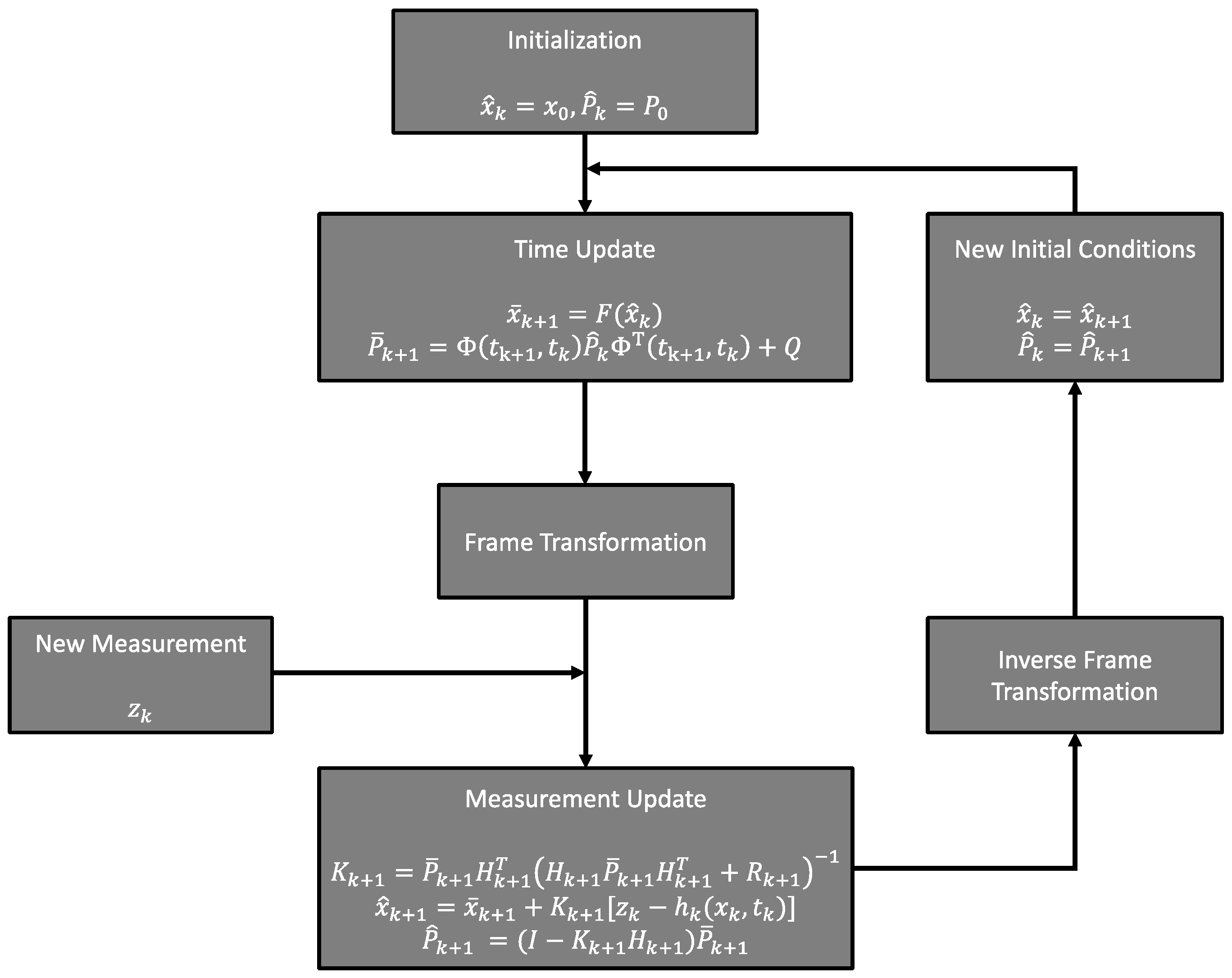
Inter-satellite data can be directly processed onboard, and the approach that is adopted to analyze these measurements is different compared to ground tracking data. To enable a real-time estimation of the spacecraft trajectory, sequential processing of the measurements acquired by the navigation system can be employed to compute a new estimate of the state vector. This estimation scheme is well-suited for real-time space applications since it is independent of the system’s state history. The Kalman filter [35] is a class of sequential processors widely used in engineering applications. If the dynamical system considered is linear and both measurement and dynamical noise models can be described by Gaussian probability density functions, the Kalman filter provides the optimal, minimum variance estimate of the parameters. The non-linearity of the dynamical equations involved in orbital dynamics requires the linearization of the system and the formulation of the problem in terms of the estimation of perturbation from a reference state. To reduce the errors associated with higher-order terms truncation in the linearization process, the reference state is updated each time a new measurement is available. This algorithm, referred to as the extended Kalman filter (EK) used in this work, and its block diagram for the autonomous navigation system is presented in Figure 1.
The non-linear dynamical model of spacecraft motion equations is described by:
where is the state vector, which consists of parameters adjusted in the filter, including spacecraft position and velocity, is the non-linear expression of the dynamical model, and is a vector that represents the process noise. We assume here that the state vector is by accounting for position and velocity of the observed spacecraft only. The measurement model is given by:
where is each inter-satellite Doppler observable acquired at time , is the non-linear measurement model, and is the observation error. We assume that both the process and observation noise are zero-mean Gaussian processes, with covariance matrices denoted as and , respectively. The process and measurement noise are,
where and are retrieved through a thorough tuning of the filter. The quality of the estimate strongly depends on the modeling of these matrices [36,37], and Section 3.2 describes the method adopted in this study to enable an accurate tuning.
Equations (1) and (2) are usually linearized by assuming that the state vector is close to a reference state. By expanding in Taylor series about the reference state and retaining only first-order terms:
where and are the Jacobian matrices of the state and inter-satellite observation model, respectively. The difference between the observed measurement acquired by the onboard system and the computed observable is the observation residual. The inter-satellite observation description and equation are provided in [22]. By accounting for the relevant dynamical and measurement effects, the residuals should resemble a white Gaussian noise associated with the measurement noise consistent with .
The EKF provides an estimate of the state and the associated covariance at each time a new measurement is available. This filter consists of two phases, a prediction (also known as time update) and a correction (measurement update). In the first phase, the state and covariance are propagated from the current time step to the next time step . If an estimate of the state is available, either from the filter initialization or estimated at the previous time step, the time update of the state is carried out by integrating the dynamical equation of the spacecraft:
The estimate of the covariance of the state is mapped out to the next time step by using the linearized expression involving the state transition matrix ,
The updated vector and associated covariance are known as predicted or a priori, since they are retrieved through the model integration. The correction phase is then carried out by refining the predicted values with the measurements collected by the intersatellite tracking system. The updated estimate of the state is:
where the Kalman gain is defined as
The estimated covariance is computed as follows,
The estimated values of state and covariance are known as posteriori estimates.
To precisely adjust the spacecraft position and velocity, both vectors are expressed in the radial-transverse-normal (RTN) reference frame centered in the spacecraft center-of-mass. The orthonormal axes of this frame are the radial direction aligned with the position vector of the spacecraft with respect to the central body, the normal direction (cross-track) parallel to the orbital angular momentum (i.e., normal to the orbital plane), and the transverse direction . Since the two spacecraft are in a coplanar orbit, the inter-satellite Doppler data are almost exclusively affected by the radial and transverse components of the position and velocity vectors, providing poor constraints on the position and velocity components normal to the orbital plane. The weak observability of these parameters can affect the estimation of the spacecraft state by introducing numerical degeneracies, leading to the divergence of the estimated parameters covariance matrix. To deal with singularity issues, we exclude the cross-track components in the estimation of the state and the covariance matrix in the spacecraft-centered radial, transverse, and normal (RTN) reference frame. The dynamical equations (Equation (5)) are integrated into the International Celestial Reference Frame (ICRF), which is inertial. Before the measurement update (Equations (7)–(9)), the propagated state is expressed in the RTN frame through the following rotation,
where is the matrix that defines the rotation from ICRF to RTN. To obtain the predicted covariance in the RTN frame, the state transition matrix must be referenced to the RTN frame through the rotation matrix :
where is a 3 3 zero matrix. The state transition matrix in RTN is:
The covariance matrix is, therefore, directly computed in the RTN frame by using Equation (9) with the state transition matrix given by Equation (12).
The correction phase then allows us to incorporate the new measurement and provide a new estimate of the state in the RTN frame. The a posteriori estimate of the state is computed by using Equation (7), which requires the Jacobian of the observation model to be expressed in the RTN frame. In this step, we only estimate the radial and transverse components of the position and velocity vectors, while the normal components are directly provided by the trajectory integration:
where , , , are the updated radial and transverse position and velocity components, and , are the cross-track components obtained from the trajectory integration. The updated state vector is then referenced to the ICRF frame and used as the new initial conditions in the subsequent time step.
The state vector only includes the position and velocity of the observer because the state of the secondary spacecraft is unobservable. The knowledge of both spacecraft trajectories can be obtained through the combination of deep space and inter-satellite tracking data with a least-squares approach [22]. The errors accumulated in the knowledge of the secondary spacecraft trajectory and of the normal component of the primary spacecraft may lead to the divergence of the sequential processor. To reduce the errors, the filter can be reinitialized by obtaining a new estimate of both the trajectories and the associated covariances through the combination of a batch of inter-satellite and ground-based tracking data [22].
We note that the weak observability of the cross-track components derives from the coplanarity of the two spacecraft orbits. Our choice of this orbital geometry is based on a mission scenario already considered for radio science investigations [24] and navigation [22] that involves the inter-satellite tracking system considered here. Changes in the orbital plane inclination between the two satellites could improve the observability of the dynamical system.
An alternative approach could be the inclusion in the filter of the cross-track components as considered parameters to account for the effects of the uncertainty in their knowledge on the other estimated parameters. However, the correlations between the R-, T-components, and the N-components computed by estimating all the parameters are close to zero. Since the cross-track state is largely uncorrelated from the radial and transverse state, this approach would lead to the same results as excluding the normal components from the estimation process.
To better understand the reliability of the state estimation from a given set of measurements, we study the observability of the system through the following matrix [38,39],
where is the dimension of the state of the system. The dynamical system is observable if the rank of the observability matrix, , is equal to . If one or more parameters are not observable by the measurements processed in the filter, the observability matrix is singular, and its rank is less than . When the system is not observable or weakly observable, the Kalman filter yields extremely large formal uncertainties, leading to unreliable estimates.
2.3. Numerical Simulation Setup
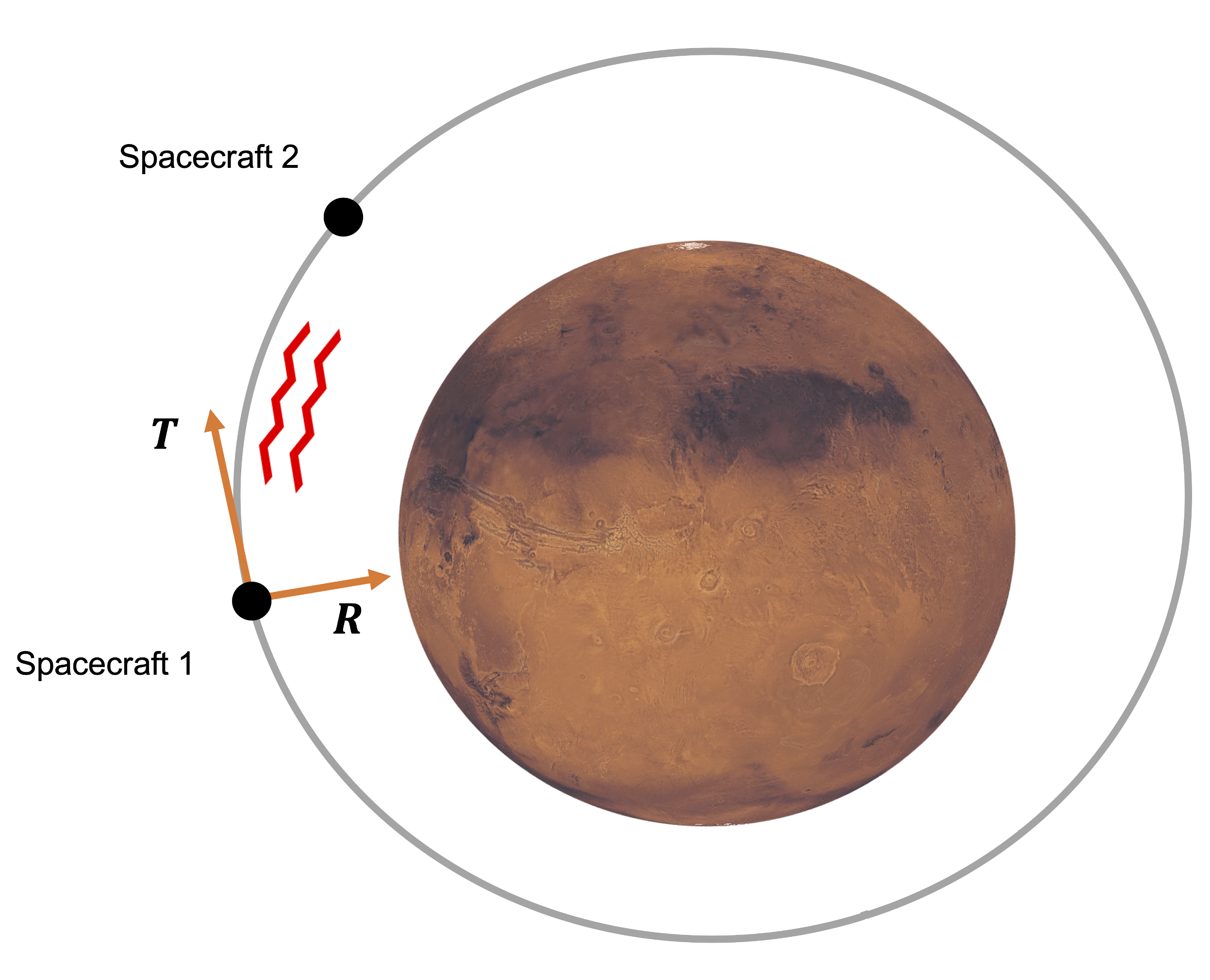
The scenario that is assumed in our numerical simulations is based on a dual-SmallSat mission [22,23,24] with a nominal orbit configuration similar to the Mars Reconnaissance Orbiter (MRO) mission [40]. This orbit is near-polar (93° inclination), with a pericenter located across Mars’ south at 250 km altitude and the apocenter at 320 km. An inter-satellite distance of 300 km is adopted to enable an accurate recovery of the static and time-varying gravity field of Mars [24]. Figure 2 shows this orbital configuration and the RTN reference frame used in the Kalman filter.
We carried out numerical simulations by assuming that the Small-Sat host onboarded a telecommunication system for inter-satellite tracking. The first step consisted of the generation of the synthetic dataset of inter-satellite Doppler measurements by simulating the reference trajectory. The dynamical model includes the central body gravity field expressed in spherical harmonics to degree and order 120 [41], the gravitational influence of the Sun and the other planets of the solar system, the solar radiation pressure, and the atmospheric drag by assuming the atmospheric density from the semi-empirical Mars Global Reference Atmospheric Model (GRAM) 2010 [42]. The spacecraft shape and thermo-optical properties are based on the MRO spacecraft design [40]. Both spacecraft are characterized by a cross-section area equal to 4 m2 and specular and diffusive reflectivity of 0.52 and 0.07. The mass of each probe is 200 kg [24]. Table 1 summarizes the properties of the dynamical and measurement models adopted in our numerical simulations.
The EKF presented in Section 2.2 is initialized by using as initial position and velocity the MRO-like reference trajectory for both observed and observer spacecraft with an initial inter-satellite distance of 300 km. The initial guess of the state vector is perturbed to account for errors in the preliminary knowledge of the spacecraft trajectory. To investigate the statistics of the Kalman filter (i.e., the initial covariance in the RTN frame , the process and measurement noise covariance and ), we proceed with the filter tuning and a thorough study of the system observability.
2.4. Filter Tuning
The tuning of the Kalman filter consists of the selection of the process and measurement noise statistics, which strongly affect the performance of the filter. The Kalman gain is controlled by the process and measurement noise covariances through Equation (8). Once a new measurement is acquired, it is combined with the dynamical model to provide an updated estimate of the system’s state and covariance. The gain of the filter opportunely scales the information provided by the new measurements with respect to the predictions retrieved by integrating the dynamical model. By increasing the elements of the observation noise covariance , the processed measurements are deweigthed, leading to lower Kalman gains. The addition of the process noise places more weight on the information given by the measurements with respect to the prediction.
We tuned the filter adopted in this work by using a trial-and-error approach. After each trial, the trajectory reconstruction error and estimated covariance are compared to determine whether the filter output is statistically consistent (i.e., errors lower than formal uncertainties). Since the observation noise affecting the inter-satellite Doppler data is directly added as white Gaussian noise in the generation of the synthetic observables, we assumed a measurement covariance of , which is as inter-satellite range-rate. Different values of were tested, but the performances of the filter are not significantly affected by the absolute value of this quantity.
The tuning of the filter is obtained by scaling the process noise covariance matrix , which is assumed to be diagonal, as follows,
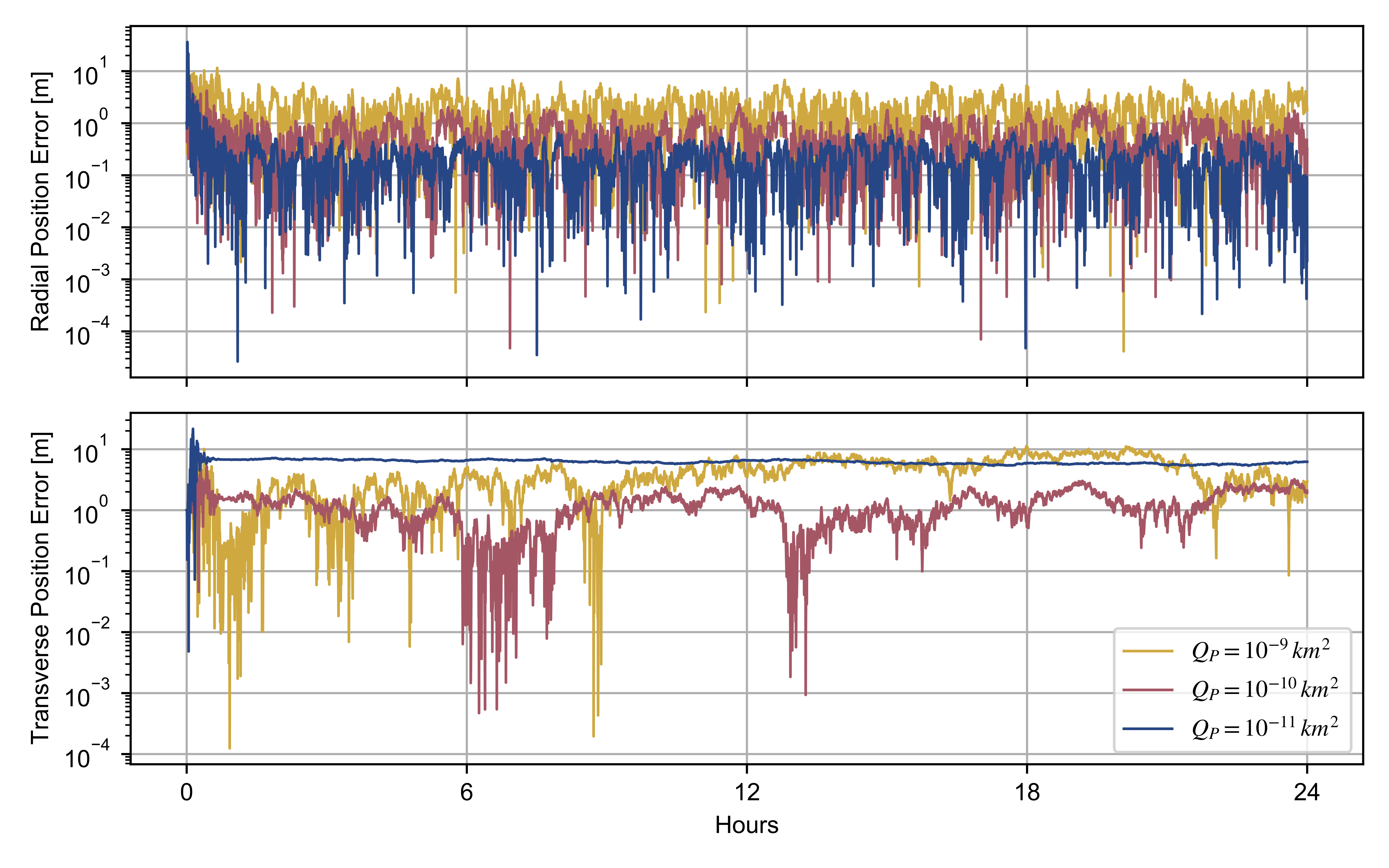
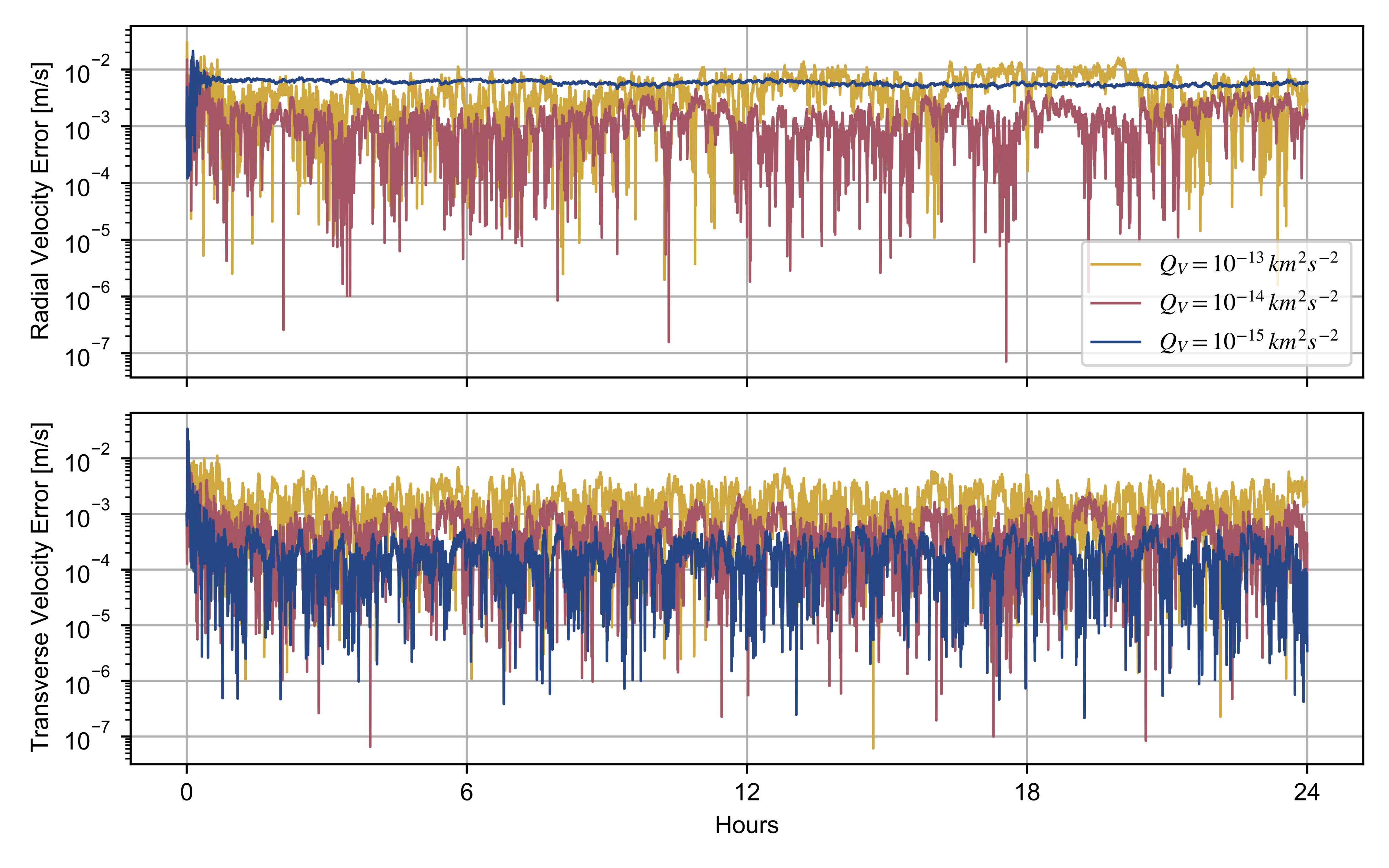
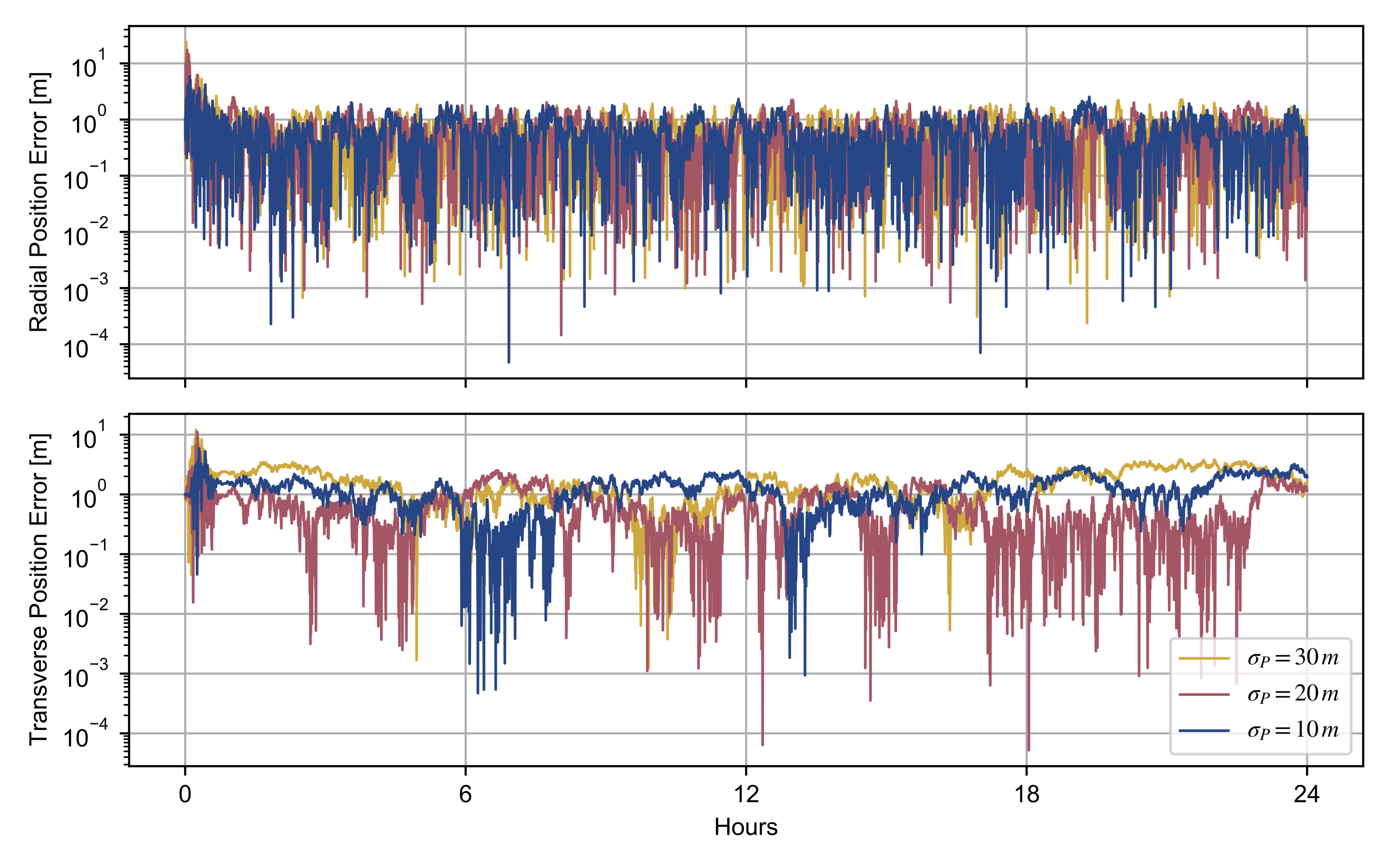
By assuming and , we studied the effects of different process noise covariances on the trajectory reconstruction of the observed spacecraft. Figure 3 and Figure 4 show the position and velocity reconstruction errors, which are the discrepancies between the simulated and adjusted trajectory, as function of and .
The pair of process noise covariances and provide more accurate adjustment of both position and velocity of the spacecraft. A lower value of enables a better determination of the radial position only, limiting an accurate retrieval of the transverse position. This filter output is explained by a significant decrease in the Kalman gain, leading to a worse transient response. A similar effect is observed in the velocity determination, although a lower prevents an accurate estimation of the radial velocity.
The initial covariance matrix has also a strong impact on the filter behavior, and it is, in general, considered an additional tuning factor. A significant difference in this matrix, with respect to the measurement and process noise, is its poor contribution to the steady-state properties of the system state. The initial covariance matrix may affect the transient response, and it is tuned by modeling it as a diagonal matrix,
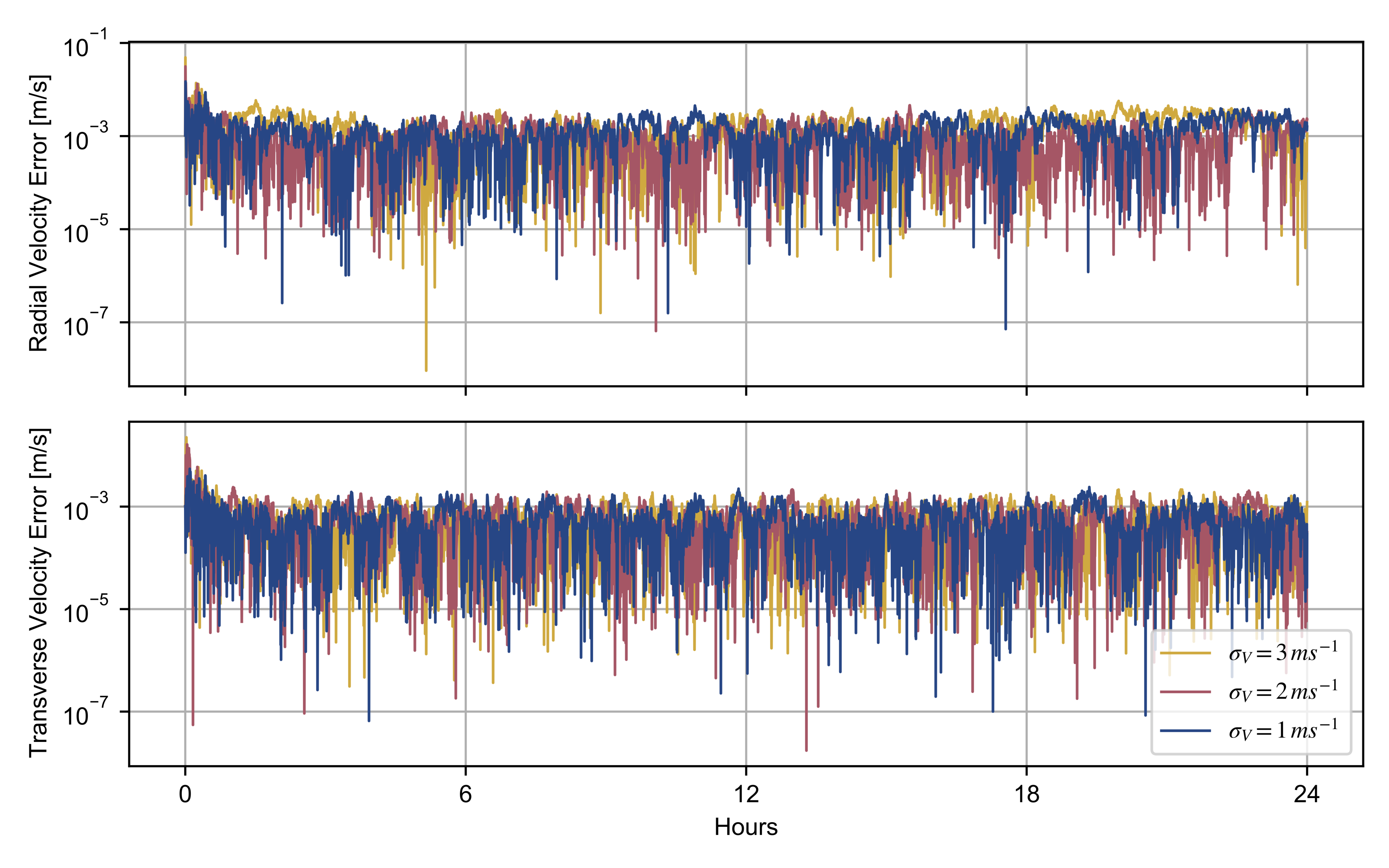
where and are the a priori uncertainties on the position and velocity components, respectively. Figure 5 and Figure 6 show the errors we obtained in the position and velocity determination with different values of the initial uncertainties.
The errors in the estimated velocity are not significantly affected by the assumed initial covariance, with a root mean square (RMS) value of for equal to , respectively. The determination of the position is more sensitive to the a priori covariance matrix , especially for the transverse direction. Since deep space tracking for the MRO spacecraft enabled accuracies of ~1 m radially and ~10–20 m along-track [43], we assumed as conservative a priori uncertainty = 20 m. This constraint in the position shows the good performances of the filter, leading to errors lower than 2 m. A looser a priori uncertainty leads to larger errors (>2 m) in the sequential reconstruction of the transverse position, suggesting that the combination of deep space and inter-satellite tracking is necessary to enhance the precise orbit determination.
3. Results
3.1. Observability of the System
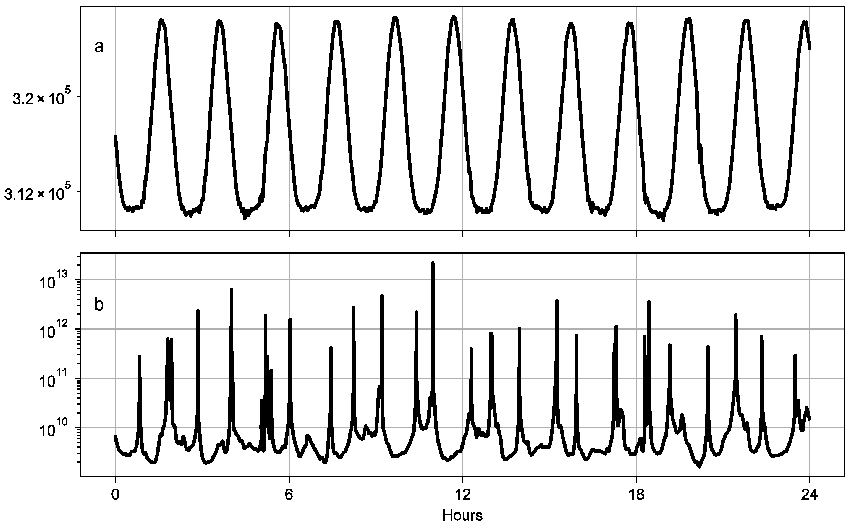
To investigate the observability of the system, we computed the observability matrix according to Equation (14). The condition number of this matrix is usually used as a metric to evaluate the observability of a system and to determine whether the state of the system can be reliably estimated through the Kalman filter [38,39,44]. The condition number is computed by implementing the estimation scheme presented in Section 2.2. We present two cases that account for radial and transverse directions only and for all three position components, including the normal direction. Figure 7 shows the temporal evolution of the observability condition number by assuming a reduced (i.e., four parameters that are position and velocity in the radial and transverse directions) and full state vector.
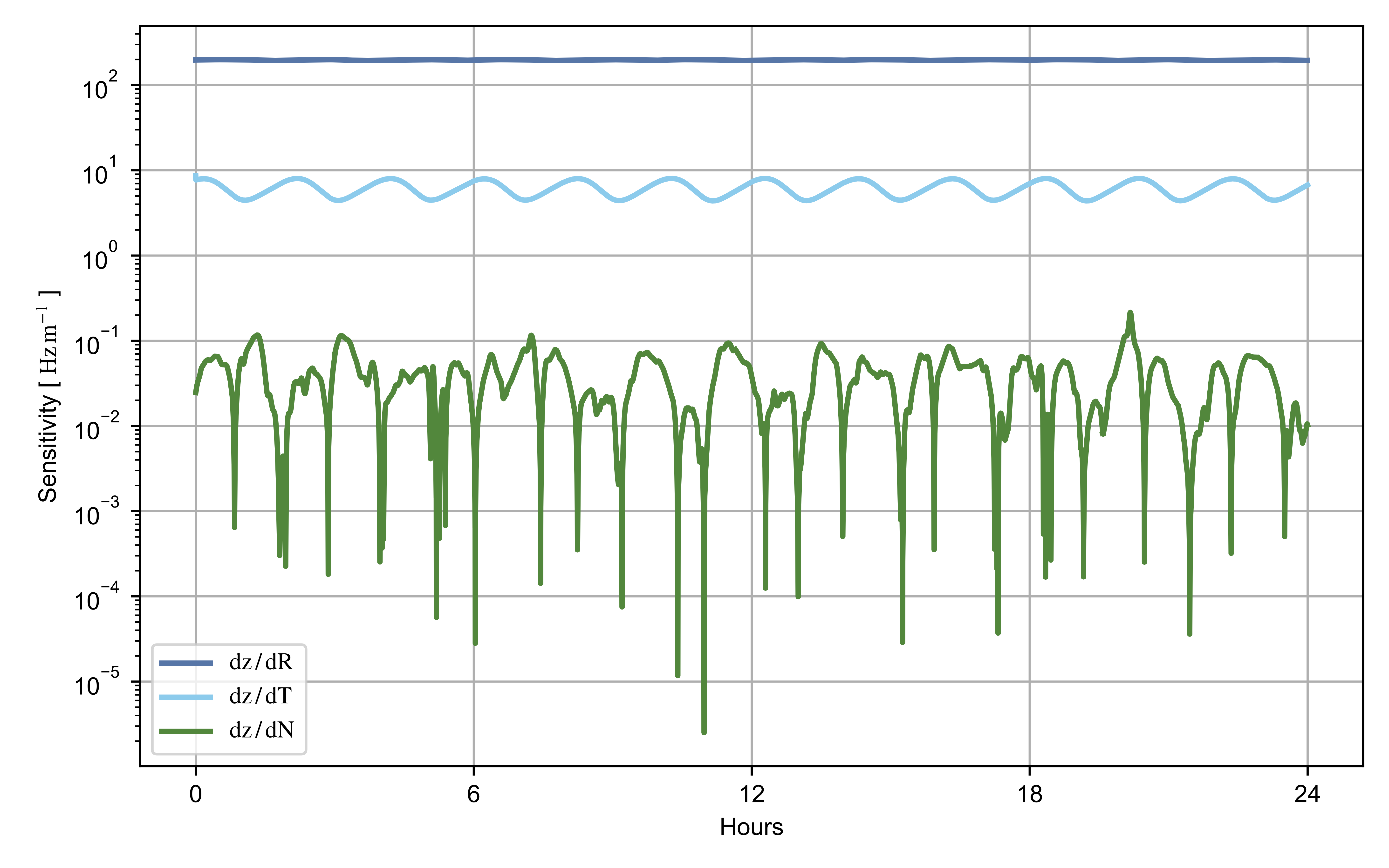
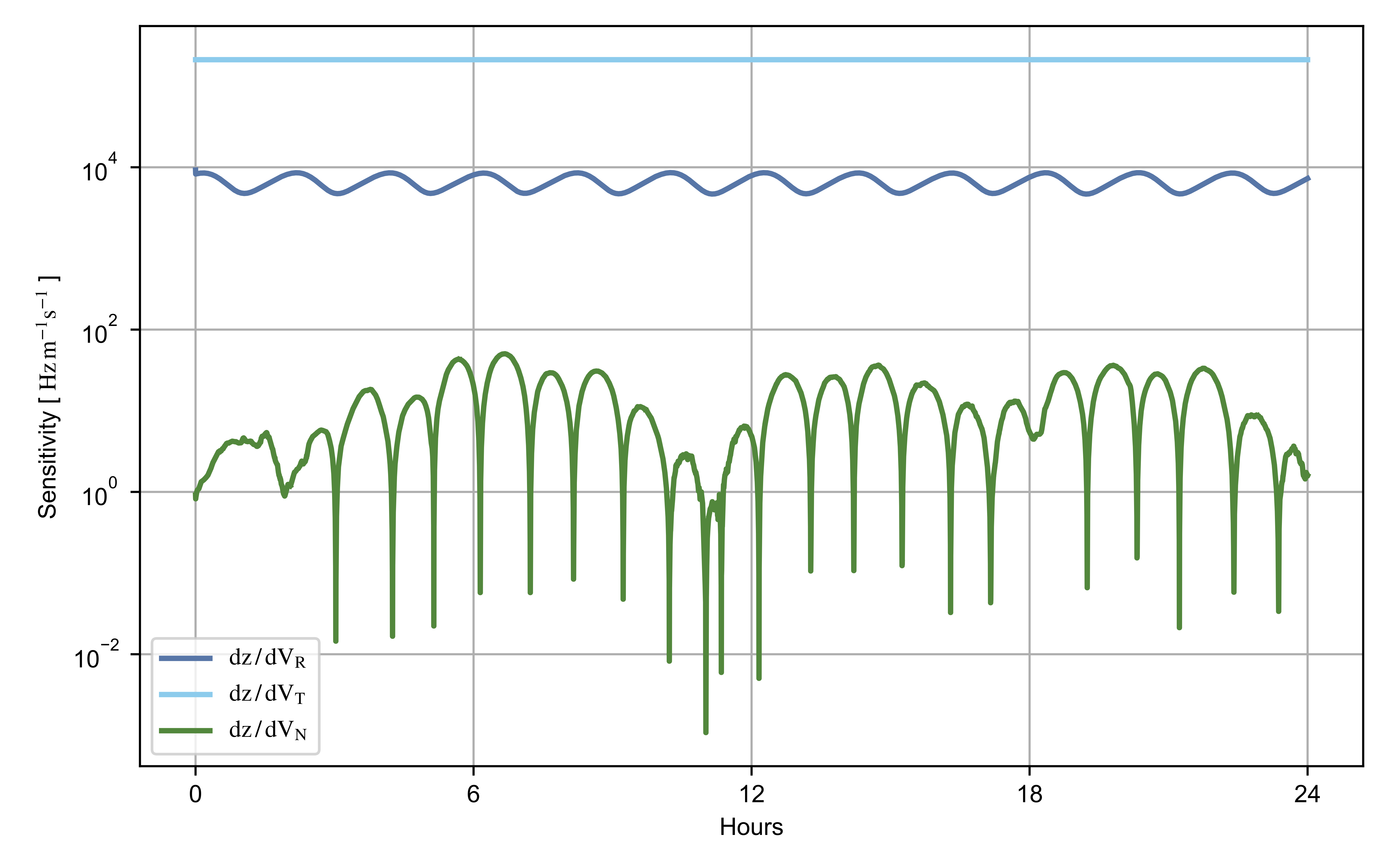
If the normal position and velocity are adjusted in the filter, the observability condition number is strongly inflated, yielding from four to seven orders of magnitude larger values compared to the estimation of radial and transverse directions only. Our results suggest that the observability matrix is close to a singularity, and the system is weakly observable. The cross-track components of position and velocity are then not observable with the inter-satellite Doppler tracking data. When including these parameters in the estimation process, unreliable estimates of the system state result from the EKF. Additional evidence that these measurements are not well-suited for the adjustment of the state normal direction is provided by the elements of the Jacobian matrix, , of the inter-satellite observation model. The partial derivatives of the observables with respect to the state information on the sensitivity of the data to the estimated parameters. Figure 8 and Figure 9 show the elements of the matrix that corresponds to the sensitivity of the inter-satellite Doppler measurements to position and velocity, respectively.
A lower sensitivity of the normal component compared to the orbital plane directions is observed in both position and velocity. This effect is caused by the coplanarity of the spacecraft orbits that prevent the inter-satellite data from constraining the state cross-track direction. This is further indicated by the anti-correlation between the condition number of the observability matrix (Figure 7b) and the sensitivity to the normal position component (Figure 8). The estimation scheme presented in this work is then used to precisely adjust the state radial and transverse directions.
3.2. Sequential Orbit Reconstruction
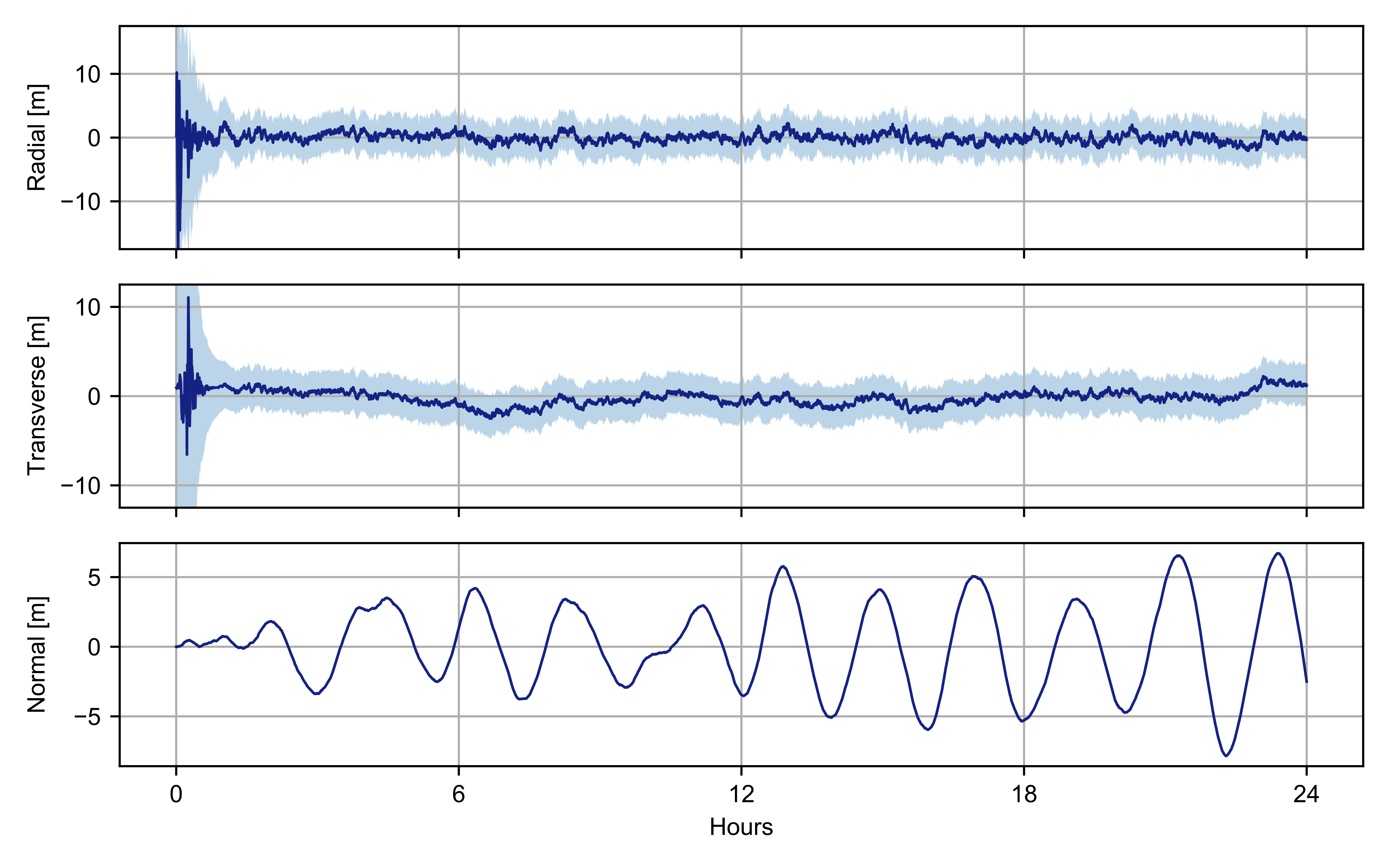
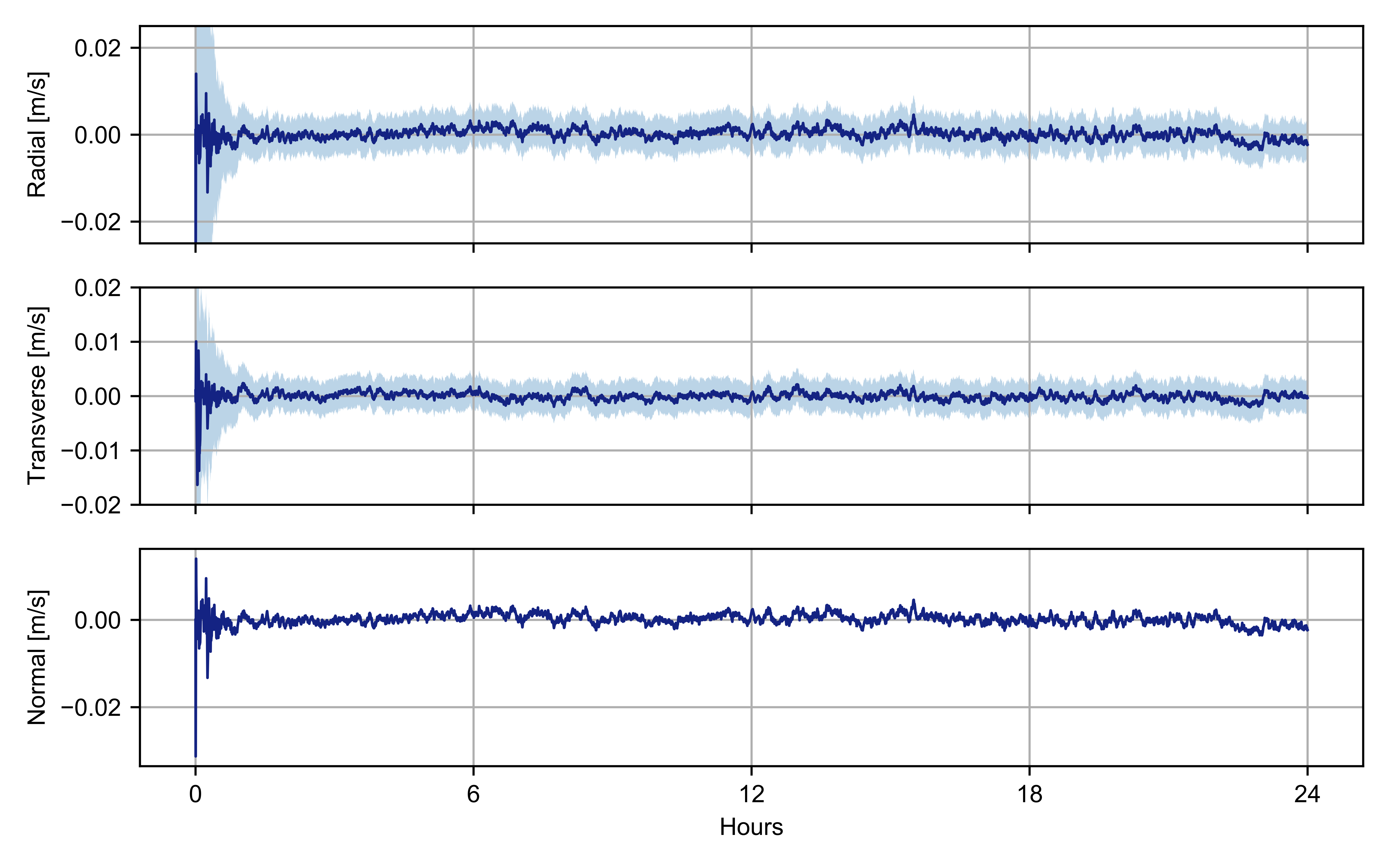
To account for errors in the initial conditions of the spacecraft state associated with the preliminary solution based on processing deep space tracking data only [22], we perturbed the initial state of the observed spacecraft by 1.5 m and 1.5 mm/s with respect to the simulated reference trajectory. The filter is then initialized with the assumptions reported in Table 2 and used to reconstruct the trajectory of the observed spacecraft by processing the inter-satellite Doppler measurements for 24 h. The measurement count time is 10 s. The position and velocity reconstruction errors with the estimated uncertainty are shown in Figure 10 and Figure 11, respectively.
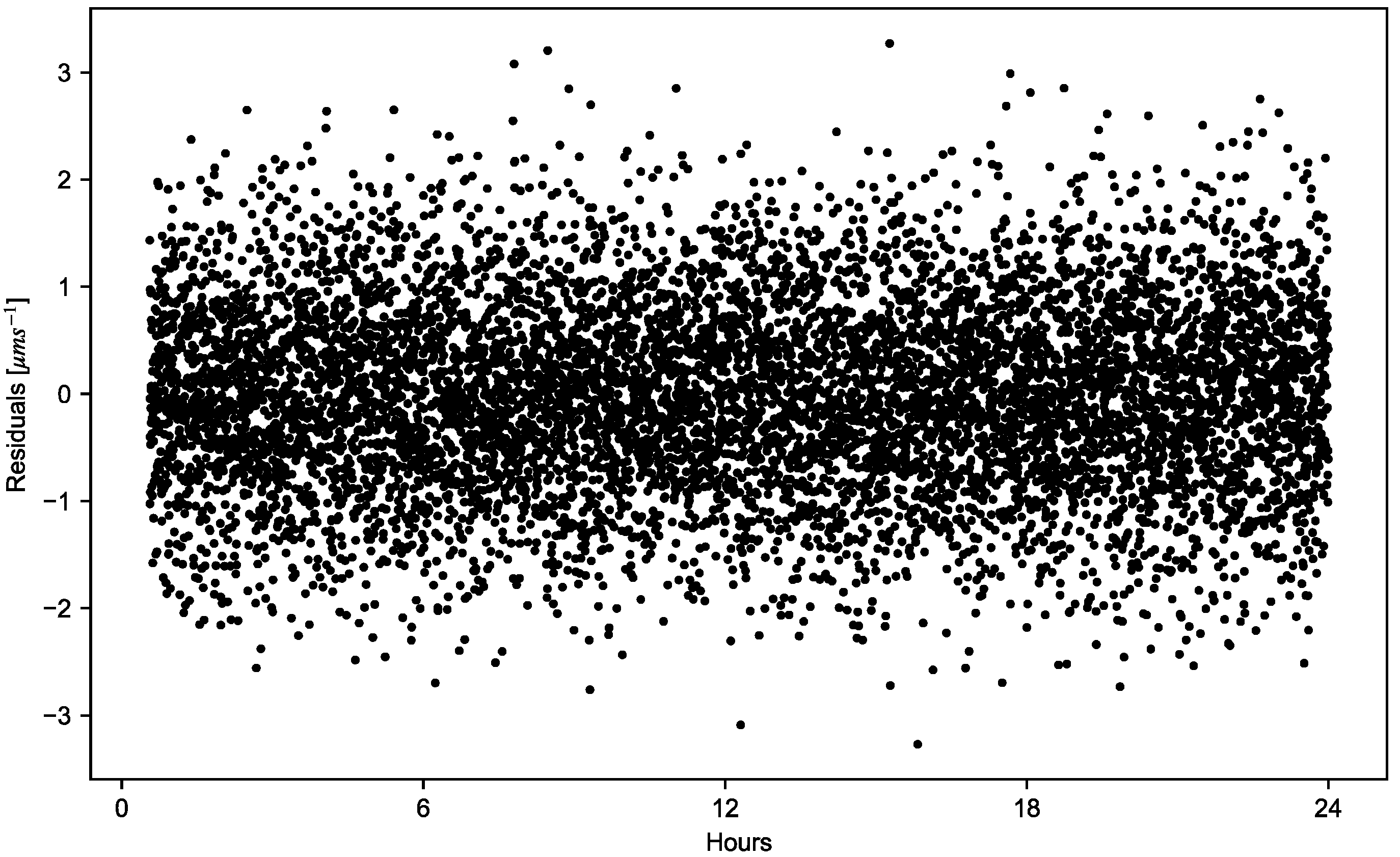
After a transient response, the Kalman filter can accurately reconstruct the trajectory of the spacecraft with position and velocity errors that are statistically consistent with the formal uncertainties. Extremely high accuracies are obtained for both radial and transverse components with three-standard-deviation formal uncertainties of ~3 and ~3 in position and velocity, respectively. Figure 12 shows the residuals of the inter-satellite measurements after the filter transient response.
Since the cross-track is not corrected with the measurements, the error affecting its knowledge grows in time. To evaluate the benefit of the navigation scheme presented here for ground operations, we extended our numerical simulations to 3 days and 7 days. The results show an error in the normal position of ~20 m and ~60 m, respectively. In this study, we did not consider any error affecting the cross-track dynamics (e.g., error on the initial normal position and velocity or mismodeling of the spacecraft dynamics). Considering such errors may lead to larger errors on the normal components. When the errors in the knowledge of the spacecraft position become large, they can be reduced by using ground-based tracking data and re-initializing the filter with the new solution.
4. Conclusions
Future space missions will require an increasing degree of autonomy to reach unexplored environments and to safely operate assets during risky science phases. The navigation of deep space probes is still exclusively based on the remote processing of ground station tracking systems, which prevent the real-time adjustment of spacecraft trajectories. A navigation scheme is elaborated by sequentially processing satellite-to-satellite Doppler measurements acquired by a sophisticated, accurate inter-satellite radio tracking system. This system was conceived for radio science investigations [22], and it can provide highly accurate navigation capabilities for both spacecraft if inter-satellite data are jointly processed with the tracking data collected by the ground stations [24]. This combination provides accurate knowledge of the initial states of both spacecraft, which can be used to initialize the navigation scheme presented here. The joint processing of inter-satellite and ground-based tracking data can be used to update the estimate of both spacecraft trajectories when they are affected by significant errors (e.g., recovery after safe mode). Although the system presented is not designed to enable fully autonomous navigation capabilities in deep space, it can significantly reduce the dependence on ground systems by providing onboard trajectory determination through sequential processing of the inter-satellite data.
To analyze the performances and functionalities of this onboard system, software to process the inter-satellite measurements was designed and implemented in this study. By adopting an extended Kalman filter scheme, we were able to study the observability and simulate the navigation accuracies expected for the proposed system. This approach is not well suited for the joint estimation of the state vectors for both observer and observed spacecraft. A precise knowledge of both spacecraft orbits can only be obtained through the combined processing of deep space and inter-satellite tracking data with a least-squares filter [24]. Our sequential algorithm allows for the retrieval of the position and velocity of the observed spacecraft only.
Because of the coplanarity of the two SmallSat orbits, the cross-track components of both position and velocity cannot be constrained with the inter-satellite measurements, as confirmed by our observability analysis of the system. This weak observability may significantly affect the estimation process, leading to numerical degeneracies and to high uncertainties regarding the observed spacecraft position and velocity. For this reason, we do not adjust the position and velocity components in the normal directions, leading to a reduced state of the system. The cross-track component is fully determined by the direct integration of the dynamical equations, and it is not corrected by the inter-satellite data. The errors that accumulate in the knowledge of the cross-track components can be reduced by periodically updating the knowledge of the spacecraft trajectory through ground-based tracking. Alternatively, additional measurements can be considered to improve the observability of the cross-track components, such as angle-based measurements provided by optical data or observations collected by radar or laser trackers onboard the primary spacecraft [45]. These measurements are more sensitive to the normal components of position and velocity than inter-satellite data and can be used to correct the errors affecting them.
Our estimation scheme provides a reliable estimate of the spacecraft state in the orbital plane components, leading to 3 − uncertainties that are ~3 m in position and 3 mm s−1 in velocity. This level of accuracy is a significant enhancement in orbit reconstruction, which is at least an order of magnitude worse with deep space tracking data only. Our results strongly support the development of an inter-satellite tracking system for navigation in deep space, leading to the extremely precise positioning of space probes across the solar system.
Author Contributions
Conceptualization, F.P. and A.G.; Investigation, F.P.; Methodology, F.P. and A.G.; Supervision, A.G.; Writing–original draft, F.P.; Writing–review & editing, A.G. All authors have read and agreed to the published version of the manuscript.
Funding
F.P. is supported by the Italian Space Agency (ASI) under contract 2021-19-HH.0.
Data Availability Statement
The trajectory kernels of the Mars Reconnaissance Orbiter are available at: https://naif.jpl.nasa.gov/pub/naif/MRO/kernels/ (accessed on 21 September 2022).
Conflicts of Interest
The authors declare no conflict of interest.
References
- Thornton, C.L.; Border, J.S. Radiometric Tracking Techniques for Deep-Space Navigation; JPL Deep Space Communications and Navigation Series; Wiley: Hoboken, NJ, USA, 2003; Volume 1, pp. 3–7. [Google Scholar]
- Esposito, P.; Alwar, V.; Demcak, S.; Graat, E.; Johnston, M.; Mase, R.A. Mars Global Surveyor: Navigation and Aerobraking at Mars. In Proceedings of the AAS/GSFC 13th International Symposium on Space Flight Dynamics, Greenbelt, MD, USA, 11–15 May 1998; Paper AAS 98-384. American Astronautical Society: San Diego, CA, USA, 1998. [Google Scholar]
- Li, S.; Cui, P. Landmark tracking based autonomous navigation schemes for landing spacecraft on asteroids. Acta Astronaut. 2008, 62, 391–403. [Google Scholar] [CrossRef]
- Kubota, T.; Hashimoto, T.; Sawai, S.; Kawaguchi, J.; Ninomiya, K.; Uo, M.; Baba, K. An autonomous navigation and guidance system for MUSES-C asteroid landing. Acta Astronaut. 2003, 52, 125–131. [Google Scholar] [CrossRef]
- Ma, X.; Fang, J.; Ning, X. An overview of the autonomous navigation for a gravity-assist interplanetary spacecraft. Prog. Aerosp. Sci. 2013, 63, 56–66. [Google Scholar] [CrossRef]
- Ou, Y.; Zhang, H.; Li, B. Absolute orbit determination using line-of-sight vector measurements between formation flying spacecraft. Astrophys. Space Sci. 2018, 363, 76. [Google Scholar] [CrossRef]
- Yu, F.; He, Z.; Xu, N. Autonomous navigation for GPS using inter-satellite ranging and relative direction measurements. Acta Astronaut. 2019, 160, 646–655. [Google Scholar] [CrossRef]
- Kai, X.; Chunling, W.; Liangdong, L. Autonomous navigation for a group of satellites with star sensors and inter-satellite links. Acta Astronaut. 2013, 86, 10–23. [Google Scholar] [CrossRef]
- Li, Y.; Zhang, A. Observability analysis and autonomous navigation for two satellites with relative position measurements. Acta Astronaut. 2019, 163, 77–86. [Google Scholar] [CrossRef]
- Lauretta, D.S.; Balram-Knutson, S.S.; Beshore, E.; Boynton, W.V.; D’Aubigny, C.D.; DellaGiustina, D.N.; Enos, H.L.; Golish, D.R.; Hergenrother, C.W.; Howell, E.S.; et al. OSIRIS-REx: Sample Return from Asteroid (101955) Bennu. Space Sci. Rev. 2017, 212, 925–984. [Google Scholar] [CrossRef] [Green Version]
- Watanabe, S.; Tsuda, Y.; Yoshikawa, M.; Tanaka, S.; Saiki, T.; Nakazawa, S. Hayabusa2 Mission Overview. Space Sci. Rev. 2017, 208, 3–16. [Google Scholar] [CrossRef]
- Lorenz, D.A.; Olds, R.; May, A.; Mario, C.; Perry, M.E.; Palmer, E.E.; Daly, M. Lessons learned from OSIRIS-REx autonomous navigation using natural feature tracking. In Proceedings of the 2017 IEEE Aerospace Conference, Big Sky, MT, USA, 4–11 March 2017; pp. 1–12. [Google Scholar] [CrossRef]
- Ogawa, N.; Terui, F.; Mimasu, Y.; Yoshikawa, K.; Ono, G.; Yasuda, S.; Matsushima, K.; Masuda, T.; Hihara, H.; Sano, J.; et al. Image-based autonomous navigation of Hayabusa2 using artificial landmarks: The design and brief in-flight results of the first landing on asteroid Ryugu. Astrodynamics 2020, 4, 89–103. [Google Scholar] [CrossRef]
- Sawai, S.; Kawaguchi, J.; Scheeres, D.J.; Yoshizawa, N.; Ogasawara, M. Development of a Target Marker for Landing on Asteroids. J. Spacecr. Rockets 2001, 38, 601–608. [Google Scholar] [CrossRef]
- Yim, J.R.; Crassidis, J.L.; Junkins, J.L. Autonomous Orbit Navigation of Interplanetary Spacecraft. In Proceedings of the Astrodynamics Specialist Conference, Denver, CO, USA, 14–17 August 2000. [Google Scholar] [CrossRef]
- Bradley, N.; Olikara, Z.; Bhaskaran, S.; Young, B. Cislunar navigation accuracy using optical observations of natural and artificial targets. J. Spacecr. Rockets 2020, 57, 777–792. [Google Scholar] [CrossRef]
- Sheikh, S.I.; Pines, D.J.; Ray, P.S.; Wood, K.S.; Lovellette, M.N.; Wolff, M.T. Spacecraft Navigation Using X-Ray Pulsars. J. Guid. Control. Dyn. 2006, 29, 49–63. [Google Scholar] [CrossRef] [Green Version]
- Kai, X.; Chunling, W.; Liangdong, L. The use of X-ray pulsars for aiding navigation of satellites in constellations. Acta Astronaut. 2009, 64, 427–436. [Google Scholar] [CrossRef]
- Wang, S.; Cui, P.; Gao, A.; Yu, Z.; Cao, M. Absolute navigation for Mars final approach using relative measurements of X-ray pulsars and Mars orbiter. Acta Astronaut. 2017, 138, 68–78. [Google Scholar] [CrossRef]
- Markley, F.L. Autonomous navigation using landmark and intersatellite data. In Proceedings of the Astrodynamics Conference, Seattle, WA, USA, 20–22 August 1984. [Google Scholar]
- Psiaki, M.L. Autonomous orbit determination for two spacecraft from relative position measurements. J. Guid. Control Dyn. 1999, 22, 305–312. [Google Scholar] [CrossRef] [Green Version]
- Genova, A.; Petricca, F. Deep-Space Navigation with Intersatellite Radio Tracking. J. Guid. Control Dyn. 2021, 44, 1068–1079. [Google Scholar] [CrossRef]
- Petricca, F.; Genova, A. ORACLE: A Dual-Smallsat Mission to Investigate the Martian Climate. In Proceedings of the 72nd International Astronautical Congress (IAC), Dubai, United Arab Emirates, 25–29 October 2021. [Google Scholar]
- Genova, A. ORACLE: A mission concept to study Mars’ climate, surface and interior. Acta Astronaut. 2020, 166, 317–329. [Google Scholar] [CrossRef]
- Wolff, M. Direct measurements of the earth’s gravitational potential using a satellite pair. J. Geophys. Res. 1969, 74, 5295–5300. [Google Scholar] [CrossRef]
- Tapley, B.D.; Bettadpur, S.; Watkins, M.; Reigber, C. The gravity recovery and climate experiment: Mission overview and early results. Geophys. Res. Lett. 2004, 31, L09607. [Google Scholar] [CrossRef] [Green Version]
- Zuber, M.T.; Smith, D.E.; Lehman, D.H.; Hoffman, T.L.; Asmar, S.W.; Watkins, M.M. Gravity Recovery and Interior Laboratory (GRAIL): Mapping the Lunar Interior from Crust to Core. Space Sci. Rev. 2013, 178, 3–24. [Google Scholar] [CrossRef] [Green Version]
- Tapley, B.; Ries, J.; Bettadpur, S.; Chambers, D.; Cheng, M.; Condi, F.; Gunter, B.; Kang, Z.; Nagel, P.; Pastor, R.; et al. GGM02—An Improved Earth Gravity Field Model from GRACE. J. Geod. 2005, 79, 467–478. [Google Scholar] [CrossRef]
- Zuber, M.T.; Smith, D.E.; Watkins, M.M.; Asmar, S.W.; Konopliv, A.S.; Lemoine, F.G.; Melosh, H.J.; Neumann, G.A.; Phillips, R.J.; Solomon, S.C.; et al. Gravity Field of the Moon from the Gravity Recovery and Interior Laboratory (GRAIL) Mission. Science 2013, 339, 668–671. [Google Scholar] [CrossRef] [Green Version]
- Kim, J.; Tapley, B.D. Simulation of Dual One-Way Ranging Measurements. J. Spacecr. Rocket. 2003, 40, 419–425. [Google Scholar] [CrossRef]
- Kruizinga, G.L.H.; Bertiger, W.I.; Harvey, N. Timing of Science Data for the GRAIL Mission; JPL Publication D-75620; California Institute of Technology: Pasadena, CA, USA, 2013. [Google Scholar]
- Asmar, S.W.; Konopliv, A.S.; Watkins, M.M.; Williams, J.G.; Park, R.S.; Kruizinga, G.; Paik, M.; Yuan, D.-N.; Fahnestock, E.; Strekalov, D.; et al. The Scientific Measurement System of the Gravity Recovery and Interior Laboratory (GRAIL) Mission. Space Sci. Rev. 2013, 178, 25–55. [Google Scholar] [CrossRef] [Green Version]
- Lemoine, F.G.; Goossens, S.; Sabaka, T.J.; Nicholas, J.B.; Mazarico, E.; Rowlands, D.D.; Loomis, B.; Chinn, D.S.; Caprette, D.S.; Neumann, G.; et al. High-Degree Gravity Models from GRAIL Primary Mission Data. J. Geophys. Res. Planets 2013, 118, 1676–1698. [Google Scholar] [CrossRef] [Green Version]
- Tapley, B.D.; Schutz, B.E.; Born, G.H. Statistical Orbit Determination; Elsevier Inc.: Amsterdam, The Netherlands, 2004. [Google Scholar]
- Kalman, R.E. A New Approach to Linear Filtering and Prediction Problems. J. Basic Eng. 1960, 82, 35–45. [Google Scholar] [CrossRef] [Green Version]
- Powell, T. Automated Tuning of an Extended Kalman Filter Using the Downhill Simplex Algorithm. J. Guid. Control. Dyn. 2002, 25, 901–908. [Google Scholar] [CrossRef]
- Bolognani, S.; Tubiana, L.; Zigliotto, M. Extended Kalman filter tuning in sensorless PMSM drives. IEEE Trans. Ind. Appl. 2003, 39, 1741–1747. [Google Scholar] [CrossRef]
- Chen, Z. Local observability and its application to multiple measurement estimation. IEEE Trans. Ind. Electron. 1991, 38, 491–496. [Google Scholar] [CrossRef]
- Chen, T.; Xu, S. Double line-of-sight measuring relative navigation for spacecraft autonomous rendezvous. Acta Astronaut. 2010, 67, 122–134. [Google Scholar] [CrossRef]
- Zurek, R.W.; Smrekar, S.E. An overview of the Mars Reconnaissance Orbiter (MRO) science mission. J. Geophys. Res. Planets 2007, 112, E05S01. [Google Scholar] [CrossRef] [Green Version]
- Genova, A.; Goossens, S.; Lemoine, F.G.; Mazarico, E.; Neumann, G.A.; Smith, D.E.; Zuber, M.T. Seasonal and static gravity field of Mars from MGS, Mars Odyssey and MRO Radio Science. Icarus 2016, 272, 228–245. [Google Scholar] [CrossRef] [Green Version]
- Justh, H.L.; Justus, C.G.; Ramey, H.S. Mars-GRAM 2010: Improving the precision of Mars-GRAM. In Proceedings of the 4th International Workshop on the Mars Atmosphere: Modelling and Observations, Paris, France, 8–11 February 2011. [Google Scholar]
- Highsmith, D.; You, T.; Demcak, S.; Graat, E.; Higa, E.; Long, S.; Bhat, R.; Mottinger, N.; Halsell, A.; Peralta, F. Mars Reconnaissance Orbiter Navigation During the Primary Science Phase. In Proceedings of the AIAA/AAS Astrodynamics Specialist Conference and Exhibit, Honolulu, HI, USA, 18–21 August 2008. [Google Scholar] [CrossRef]
- Chen, Z.; Jiang, K.; Hung, J.C. Local observability matrix and its application to observability analyses. In Proceedings of the IECON ‘90: 16th Annual Conference of IEEE Industrial Electronics Society, Pacific Grove, CA, USA, 27–30 November 1990; Volume 1, pp. 100–103. [Google Scholar] [CrossRef]
- Muller, E.S.; Kachmar, P.M. A New Approach to On-Board Orbit Navigation. Navigation 1971, 18, 369–385. [Google Scholar] [CrossRef]
Figure 1.
Block diagram of the extended Kalman filter implementation for the autonomous navigation system presented in this work.
Figure 1.
Block diagram of the extended Kalman filter implementation for the autonomous navigation system presented in this work.

Figure 2.
Orbital configuration of the dual-SmallSat mission and the orbital RTN frame. The R and T vectors denote the radial and transverse directions, and the cross-track direction is normal to the orbital plane.
Figure 2.
Orbital configuration of the dual-SmallSat mission and the orbital RTN frame. The R and T vectors denote the radial and transverse directions, and the cross-track direction is normal to the orbital plane.

Figure 3.
Radial and transverse position reconstruction errors of the observed spacecraft for different values of the process noise covariance, with and , .
Figure 3.
Radial and transverse position reconstruction errors of the observed spacecraft for different values of the process noise covariance, with and , .

Figure 4.
Radial and transverse velocity reconstruction errors of the observed spacecraft for different values of the process noise covariance, with and , .
Figure 4.
Radial and transverse velocity reconstruction errors of the observed spacecraft for different values of the process noise covariance, with and , .

Figure 5.
Radial and transverse position reconstruction errors for different values of the initial covariance, with and , .
Figure 5.
Radial and transverse position reconstruction errors for different values of the initial covariance, with and , .

Figure 6.
Radial and transverse velocity reconstruction errors for different values of the initial covariance, with and , .
Figure 6.
Radial and transverse velocity reconstruction errors for different values of the initial covariance, with and , .

Figure 7.
Condition number of the observability matrix when (a) only radial and transverse position are estimated (b) the normal components are included in the estimation.
Figure 7.
Condition number of the observability matrix when (a) only radial and transverse position are estimated (b) the normal components are included in the estimation.

Figure 8.
Sensitivity of the intersatellite Doppler data to the position components.

Figure 9.
Sensitivity of the inter-satellite Doppler data to the velocity components.

Figure 10.
Position reconstruction errors in the RTN frame (blue line) and estimated 3- uncertainties (shaded area).
Figure 10.
Position reconstruction errors in the RTN frame (blue line) and estimated 3- uncertainties (shaded area).

Figure 11.
Velocity reconstruction errors in the RTN frame (blue line) and estimated 3- uncertainties (shaded area).
Figure 11.
Velocity reconstruction errors in the RTN frame (blue line) and estimated 3- uncertainties (shaded area).

Figure 12.
Residuals of the inter-satellite measurements.


Table 1.
Properties of the dynamical and measurement models.
| Dynamical Models | Gravity Field | GMM-3 to degree and order 120 [41] |
| Atmospheric Drag | Mars GRAM 2010 [42] | |
| Solar Radiation Pressure | Cross-sectional area 4 m2 Specular and diffusive reflectivity 0.52 and 0.07 | |
| Spacecraft Mass | 200 kg | |
| Measurement Models | Intersatellite Distance | 300 km |
| Data Noise | ||
| Data Count Time | 10 s |
Table 2.
Setup of the Kalman filter.
| Parameter | Value | |
|---|---|---|
| Initial Covariance Matrix | ||
| Process Noise | ||
| Observation Noise |
Publisher’s Note: MDPI stays neutral with regard to jurisdictional claims in published maps and institutional affiliations. |
© 2022 by the authors. Licensee MDPI, Basel, Switzerland. This article is an open access article distributed under the terms and conditions of the Creative Commons Attribution (CC BY) license (https://creativecommons.org/licenses/by/4.0/).
Share and Cite
MDPI and ACS Style
Petricca, F.; Genova, A. Sequential Processing of Inter-Satellite Doppler Tracking for a Dual-Spacecraft Configuration. Remote Sens. 2022, 14, 5383. https://0-doi-org.brum.beds.ac.uk/10.3390/rs14215383
AMA Style
Petricca F, Genova A. Sequential Processing of Inter-Satellite Doppler Tracking for a Dual-Spacecraft Configuration. Remote Sensing. 2022; 14(21):5383. https://0-doi-org.brum.beds.ac.uk/10.3390/rs14215383
Chicago/Turabian StylePetricca, Flavio, and Antonio Genova. 2022. "Sequential Processing of Inter-Satellite Doppler Tracking for a Dual-Spacecraft Configuration" Remote Sensing 14, no. 21: 5383. https://0-doi-org.brum.beds.ac.uk/10.3390/rs14215383
Note that from the first issue of 2016, this journal uses article numbers instead of page numbers. See further details here.