
Detecting the Greatest Changes in Global Satellite-Based Precipitation Observations
 ,
,  , , and
Abstract
:
1. Introduction
2. Materials and Methods
2.1. Data Sources
2.2. Methods
2.2.1. Breakpoint Detection
2.2.2. Data Preprocessing
2.2.3. Precipitation Changes at Global, Continental, and Climate Zone Scales
3. Results
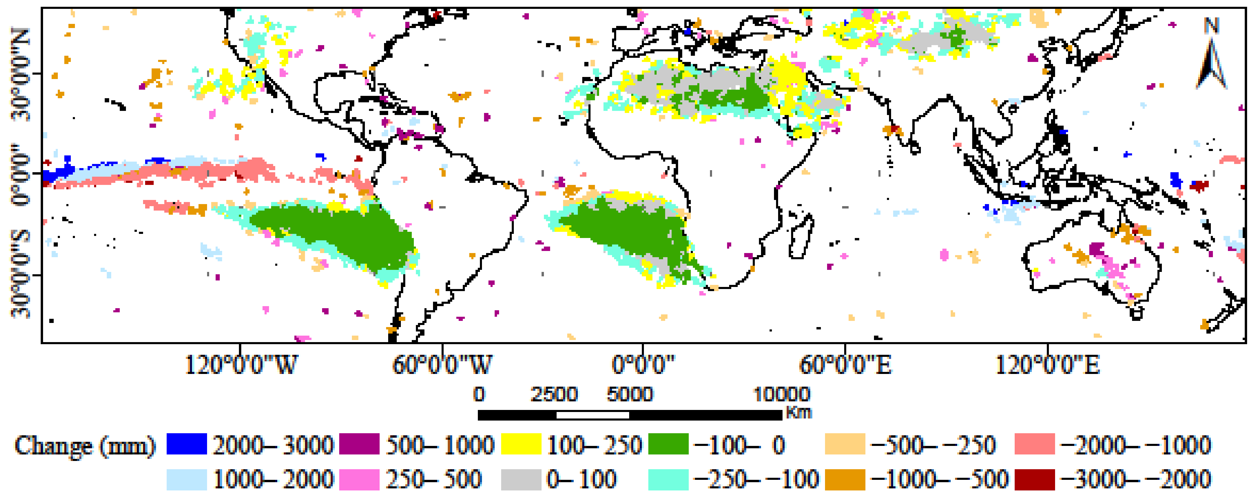
3.1. Global Scale
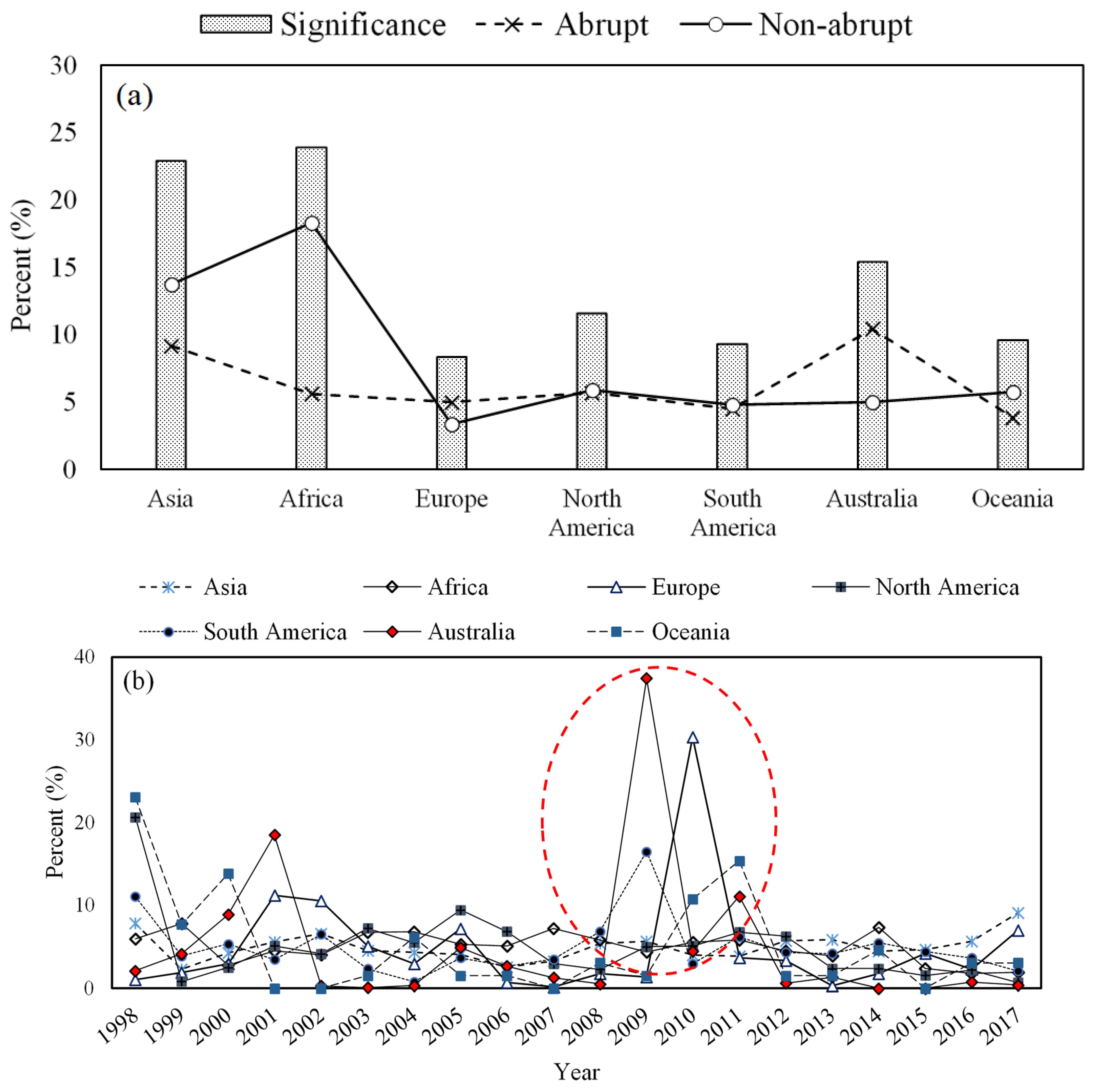
3.2. Continental Scale
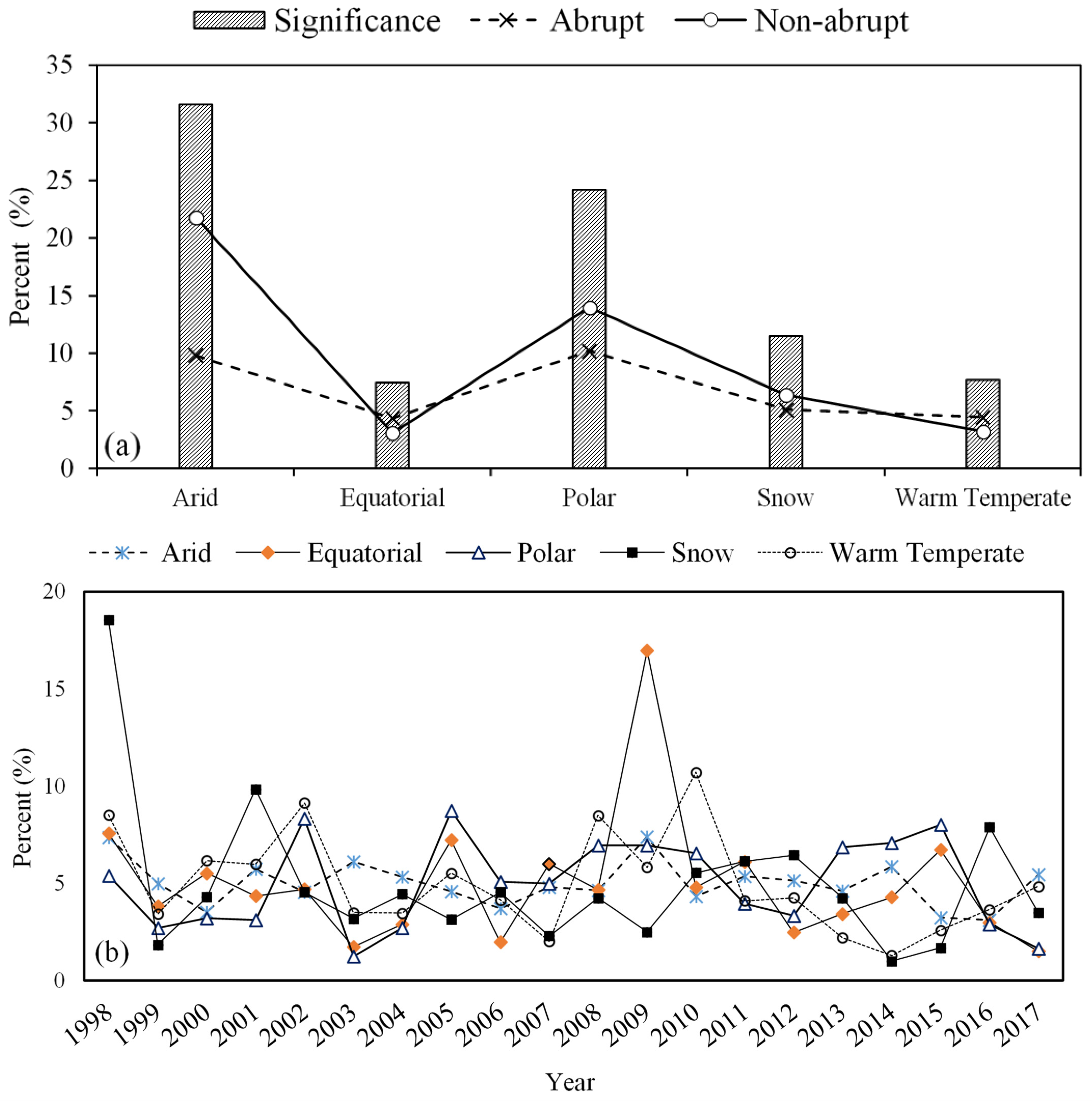
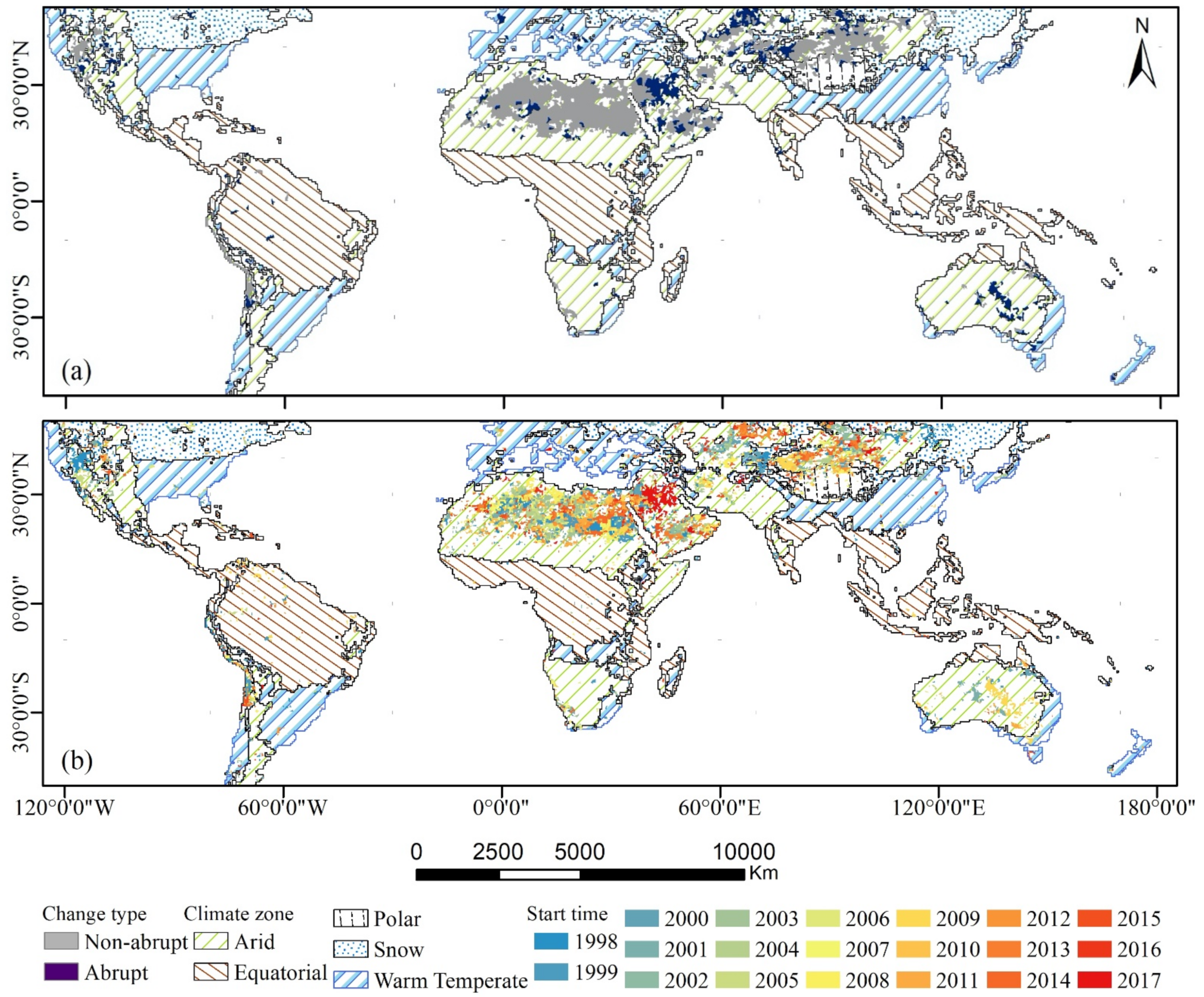
3.3. Climate Zone Scale
4. Discussion
4.1. Precipitation Changes at Global Scale
4.2. Precipitation Changes at the Continental and Climate Scales
5. Conclusions
Author Contributions
Funding
Data Availability Statement
Acknowledgments
Conflicts of Interest
References
- Longobardi, A.; Villani, P. Trend analysis of annual and seasonal rainfall time series in the Mediterranean area. Int. J. Climatol. 2010, 30, 1538–1546. [Google Scholar] [CrossRef]
- Trenberth, K.E. Changes in precipitation with climate change. Clim. Res. 2011, 47, 123–138. [Google Scholar] [CrossRef] [Green Version]
- Adler, R.F.; Gu, G.; Sapiano, M.; Wang, J.-J.; Huffman, G.J. Global precipitation: Means, variations and trends during the satellite era (1979–2014). Surv. Geophys. 2017, 38, 679–699. [Google Scholar] [CrossRef] [Green Version]
- Donat, M.G.; Lowry, A.L.; Alexander, L.V.; O’Gorman, P.A.; Maher, N. Addendum: More extreme precipitation in the world’s dry and wet regions. Nat. Clim. Change 2017, 7, 154–158. [Google Scholar] [CrossRef] [Green Version]
- Alexander, L.V.; Zhang, X.; Peterson, T.C.; Caesar, J.; Gleason, B.; Klein Tank, A.; Haylock, M.; Collins, D.; Trewin, B.; Rahimzadeh, F. Global observed changes in daily climate extremes of temperature and precipitation. J. Geophys. Res. Atmos. 2006, 111, 1042–1063. [Google Scholar] [CrossRef] [Green Version]
- Westra, S.; Alexander, L.V.; Zwiers, F.W. Global increasing trends in annual maximum daily precipitation. J. Clim. 2013, 26, 3904–3918. [Google Scholar] [CrossRef] [Green Version]
- Kharin, V.V.; Zwiers, F.W.; Zhang, X.; Wehner, M. Changes in temperature and precipitation extremes in the CMIP5 ensemble. Clim. Change 2013, 119, 345–357. [Google Scholar] [CrossRef]
- Sillmann, J.; Kharin, V.V.; Zwiers, F.; Zhang, X.; Bronaugh, D. Climate extremes indices in the CMIP5 multimodel ensemble: Part 2. Future climate projections. J. Geophys. Res. Atmos. 2013, 118, 2473–2493. [Google Scholar] [CrossRef]
- Donat, M.; Alexander, L.V.; Yang, H.; Durre, I.; Vose, R.; Dunn, R.J.; Willett, K.M.; Aguilar, E.; Brunet, M.; Caesar, J. Updated analyses of temperature and precipitation extreme indices since the beginning of the twentieth century: The HadEX2 dataset. J. Geophys. Res. Atmos. 2013, 118, 2098–2118. [Google Scholar] [CrossRef] [Green Version]
- Zhang, S.H.; Zhang, P.Y. Abrupt change study in climate change. Adv. Earth Sci. 1989, 3, 47–54. [Google Scholar]
- Buishand, T. Tests for detecting a shift in the mean of hydrological time series. J. Hydrol. 1984, 73, 51–69. [Google Scholar] [CrossRef]
- Reeves, J.; Chen, J.; Wang, X.; Lund, R.; Lu, Q. A review and comparison of climate control data for climate data. J. Appl. Meteorol. Clim. 2007, 46, 900–915. [Google Scholar] [CrossRef]
- Zhao, C.; Cui, Y.; Zhou, X.; Wang, Y. Evaluation of performance of different methods in detecting abrupt climate changes. Discret. Dyn. Nat. Soc. 2016, 2016, 5898697. [Google Scholar] [CrossRef] [Green Version]
- Lund, R.; Reeves, J. Detection of undocumented changepoints: A revision of the two-phase regression model. J. Clim. 2002, 15, 2547–2554. [Google Scholar] [CrossRef]
- Seidou, O.; Ouarda, T.B. Recursion-based multiple changepoint detection in multiple linear regression and application to river streamflows. Water Resour. Res. 2007, 43, W07404. [Google Scholar] [CrossRef] [Green Version]
- Wang, X.L. Comments on “Detection of undocumented changepoints: A revision of the two-phase regression model”. J. Clim. 2003, 16, 3383–3385. [Google Scholar] [CrossRef]
- Worsley, K. On the likelihood ratio test for a shift in location of normal populations. J. Am. Stat. Assoc. 1979, 74, 365–367. [Google Scholar]
- Buishand, T.A. Some methods for testing the homogeneity of rainfall records. J. Hydrol. 1982, 58, 11–27. [Google Scholar] [CrossRef]
- Pettitt, A.N. A non-parametric approach to the change-point problem. J. R. Stat. Soc. Ser. C 1979, 28, 126–135. [Google Scholar] [CrossRef]
- Alexandersson, H. A homogeneity test applied to precipitation data. J. Climatol. 1986, 6, 661–675. [Google Scholar] [CrossRef]
- Hsu, K.-C.; Li, S.-T. Clustering spatial–temporal precipitation data using wavelet transform and self-organizing map neural network. Adv. Water Resour. 2010, 33, 190–200. [Google Scholar] [CrossRef]
- Vincent, L.A. A technique for the identification of inhomogeneities in Canadian temperature series. J. Clim. 1998, 11, 1094–1104. [Google Scholar] [CrossRef]
- Kazemzadeh, M.; Malekian, A. Homogeneity analysis of streamflow records in arid and semi-arid regions of northwestern Iran. J. Arid Land 2018, 10, 493–506. [Google Scholar] [CrossRef] [Green Version]
- McCuen, R.H. Modeling Hydrologic Change: Statistical Methods; CRC Press: Boca Raton, FL, USA, 2016. [Google Scholar]
- Jamali, S.; Jönsson, P.; Eklundh, L.; Ardö, J.; Seaquist, J. Detecting changes in vegetation trends using time series segmentation. Remote Sens. Environ. 2015, 156, 182–195. [Google Scholar] [CrossRef]
- Schwarz, G. Estimating the dimension of a model. Ann. Stat. 1978, 6, 461–464. [Google Scholar] [CrossRef]
- Rousseeuw, P.J.; Leroy, A.M. Robust Regression and Outlier Detection; John Wiley & Sons Inc.: New York, NY, USA, 1987. [Google Scholar]
- Lenderink, G.; Van Meijgaard, E. Increase in hourly precipitation extremes beyond expectations from temperature changes. Nat. Geosci. 2008, 1, 511–514. [Google Scholar] [CrossRef]
- O’Gorman, P.A. Sensitivity of tropical precipitation extremes to climate change. Nat. Geosci. 2012, 5, 697–700. [Google Scholar] [CrossRef]
- Huffman, G.; Adler, R.; Bolvin, D.; Gu, G.; Nelkin, E.; Bowman, K.; Hong, Y.; Stocker, E.; Wolff, D. The TRMM multi-satellite precipitation analysis: Quasi-global, multi-year, combined sensor precipitation estimates at fine scales. J. Hydrometeorol. 2007, 8, 28–55. [Google Scholar] [CrossRef]
- Kummerow, C.; Simpson, J.; Thiele, O.; Barnes, W.; Chang, A.; Stocker, E.; Adler, R.; Hou, A.; Kakar, R.; Wentz, F. The status of the Tropical Rainfall Measuring Mission (TRMM) after two years in orbit. J. Appl. Meteorol. 2000, 39, 1965–1982. [Google Scholar] [CrossRef]
- Huffman, G.J.; Adler, R.F.; Bolvin, D.T.; Nelkin, E.J. The TRMM multi-satellite precipitation analysis (TMPA). In Satellite Rainfall Applications for Surface Hydrology; Springer: Berlin/Heidelberg, Germany, 2010; pp. 3–22. [Google Scholar]
- Belete, M.; Deng, J.; Wang, K.; Zhou, M.; Zhu, E.; Shifaw, E.; Bayissa, Y. Evaluation of satellite rainfall products for modeling water yield over the source region of Blue Nile Basin. Sci. Total Environ. 2020, 708, 134834. [Google Scholar] [CrossRef]
- Huffman, G.J.; Bolvin, D.T.; Braithwaite, D.; Hsu, K.-L.; Joyce, R.J.; Kidd, C.; Nelkin, E.J.; Sorooshian, S.; Stocker, E.F.; Tan, J. Integrated multi-satellite retrievals for the global precipitation measurement (GPM) mission (IMERG). In Satellite Precipitation Measurement; Springer: Berlin/Heidelberg, Germany, 2020; pp. 343–353. [Google Scholar]
- Huffman, G.J.; Bolvin, D.T. TRMM and Other Data Precipitation Data Set Documentation; NASA: Greenbelt, MD, USA, 2013; Volume 28.
- Huffman, G.J. The Transition in Multi-Satellite Products from TRMM to GPM (TMPA to IMERG). 2016. Algorithm Information Document. Available online: https://docserver.gesdisc.eosdis.nasa.gov/public/project/GPM/TMPA-to-IMERG_transition.pdf (accessed on 2 November 2021).
- Kazemzadeh, M.; Hashemi, H.; Jamali, S.; Uvo, C.B.; Berndtsson, R.; Huffman, G.J. Linear and Nonlinear Trend Analyzes in Global Satellite-Based Precipitation, 1998–2017. Earths Future 2021, 9, e2020EF001835. [Google Scholar] [CrossRef]
- Hashemi, H.; Fayne, J.; Lakshmi, V.; Huffman, G.J. Very high resolution, altitude-corrected, TMPA-based monthly satellite precipitation product over the CONUS. Sci. Data 2020, 7, 74. [Google Scholar] [CrossRef] [PubMed]
- Hashemi, H.; Nordin, M.; Lakshmi, V.; Huffman, G.J.; Knight, R. Bias correction of long-term satellite monthly precipitation product (TRMM 3B43) over the conterminous United States. J. Hydrometeorol. 2017, 18, 2491–2509. [Google Scholar] [CrossRef]
- Prat, O.P.; Nelson, B.R. Characteristics of annual, seasonal, and diurnal precipitation in the Southeastern United States derived from long-term remotely sensed data. Atmos. Res. 2014, 144, 4–20. [Google Scholar] [CrossRef]
- Qiao, L.; Hong, Y.; Chen, S.; Zou, C.B.; Gourley, J.J.; Yong, B. Performance assessment of the successive Version 6 and Version 7 TMPA products over the climate-transitional zone in the southern Great Plains, USA. J. Hydrol. 2014, 513, 446–456. [Google Scholar] [CrossRef]
- Zhao, T.; Yatagai, A. Evaluation of TRMM 3B42 product using a new gauge-based analysis of daily precipitation over China. Int. J. Climatol. 2014, 34, 2749–2762. [Google Scholar] [CrossRef]
- Brown, J.E. An analysis of the performance of hybrid infrared and microwave satellite precipitation algorithms over India and adjacent regions. Remote Sens. Environ. 2006, 101, 63–81. [Google Scholar] [CrossRef]
- Mondal, A.; Lakshmi, V.; Hashemi, H. Intercomparison of trend analysis of multisatellite monthly precipitation products and gauge measurements for river basins of India. J. Hydrol. 2018, 565, 779–790. [Google Scholar] [CrossRef]
- Prakash, S.; Mitra, A.K.; Pai, D.; AghaKouchak, A. From TRMM to GPM: How well can heavy rainfall be detected from space? Adv. Water Resour. 2016, 88, 1–7. [Google Scholar] [CrossRef]
- Huang, Y.; Chen, S.; Cao, Q.; Hong, Y.; Wu, B.; Huang, M.; Qiao, L.; Zhang, Z.; Li, Z.; Li, W. Evaluation of version-7 TRMM multi-satellite precipitation analysis product during the Beijing extreme heavy rainfall event of 21 July 2012. Water 2013, 6, 32–44. [Google Scholar] [CrossRef] [Green Version]
- Li, X.-H.; Zhang, Q.; Xu, C.-Y. Suitability of the TRMM satellite rainfalls in driving a distributed hydrological model for water balance computations in Xinjiang catchment, Poyang lake basin. J. Hydrol. 2012, 426, 28–38. [Google Scholar] [CrossRef]
- Darand, M.; Amanollahi, J.; Zandkarimi, S. Evaluation of the performance of TRMM Multi-satellite Precipitation Analysis (TMPA) estimation over Iran. Atmos. Res. 2017, 190, 121–127. [Google Scholar] [CrossRef]
- Javanmard, S.; Yatagai, A.; Nodzu, M.; BodaghJamali, J.; Kawamoto, H. Comparing high-resolution gridded precipitation data with satellite rainfall estimates of TRMM_3B42 over Iran. Adv. Geosci. 2010, 25, 119–125. [Google Scholar] [CrossRef] [Green Version]
- Moazami, S.; Golian, S.; Hong, Y.; Sheng, C.; Kavianpour, M.R. Comprehensive evaluation of four high-resolution satellite precipitation products under diverse climate conditions in Iran. Hydrol. Sci. J. 2016, 61, 420–440. [Google Scholar] [CrossRef]
- Jamandre, C.; Narisma, G.T. Spatio-temporal validation of satellite-based rainfall estimates in the Philippines. Atmos. Res. 2013, 122, 599–608. [Google Scholar] [CrossRef]
- Dinku, T.; Ceccato, P.; Grover-Kopec, E.; Lemma, M.; Connor, S.; Ropelewski, C. Validation of satellite rainfall products over East Africa’s complex topography. Int. J. Remote Sens. 2007, 28, 1503–1526. [Google Scholar] [CrossRef]
- Tan, M.L. Assessment of TRMM product for precipitation extreme measurement over the Muda River Basin, Malaysia. HydroResearch 2019, 2, 69–75. [Google Scholar] [CrossRef]
- Houghton, J.T.; Ding, Y.; Griggs, D.J.; Noguer, M.; van der Linden, P.J.; Dai, X.; Maskell, K.; Johnson, C. Climate Change 2001: The Scientific Basis: Contribution of Working Group I to the Third Assessment Report of the Intergovernmental Panel on Climate Change; Cambridge University Press: Cambridge, UK, 2001. [Google Scholar]
- Kottek, M.; Grieser, J.; Beck, C.; Rudolf, B.; Rubel, F. World map of the Köppen-Geiger climate classification updated. Meteorol. Z. 2006, 15, 259–263. [Google Scholar] [CrossRef]
- Rubel, F.; Kottek, M. Observed and projected climate shifts 1901–2100 depicted by world maps of the Köppen-Geiger climate classification. Meteorol. Z. 2010, 19, 135–141. [Google Scholar] [CrossRef] [Green Version]
- Chen, Y.; Deng, H.; Li, B.; Li, Z.; Xu, C. Abrupt change of temperature and precipitation extremes in the arid region of Northwest China. Quat. Int. 2014, 336, 35–43. [Google Scholar] [CrossRef]
- Sokol Jurković, R.; Pasarić, Z. Spatial variability of annual precipitation using globally gridded data sets from 1951 to 2000. Int. J. Climatol. 2013, 33, 690–698. [Google Scholar] [CrossRef]
- Lausier, A.M.; Jain, S. Diversity in global patterns of observed precipitation variability and change on river basin scales. Clim. Change 2018, 149, 261–275. [Google Scholar] [CrossRef]
- Dore, M.H. Climate change and changes in global precipitation patterns: What do we know? Environ. Int. 2005, 31, 1167–1181. [Google Scholar] [CrossRef] [PubMed]
- Liu, B.; Xu, M.; Henderson, M. Where have all the showers gone? Regional declines in light precipitation events in China, 1960–2000. Int. J. Climatol. 2011, 31, 1177–1191. [Google Scholar] [CrossRef]
- Ma, S.; Zhou, T.; Dai, A.; Han, Z. Observed changes in the distributions of daily precipitation frequency and amount over China from 1960 to 2013. J. Clim. 2015, 28, 6960–6978. [Google Scholar] [CrossRef]
- Wen, G.; Huang, G.; Tao, W.; Liu, C. Observed trends in light precipitation events over global land during 1961–2010. Theor. Appl. Climatol. 2016, 125, 161–173. [Google Scholar] [CrossRef]
- Yang, T.; Li, Q.; Chen, X.; De Maeyer, P.; Yan, X.; Liu, Y.; Zhao, T.; Li, L. Spatiotemporal variability of the precipitation concentration and diversity in Central Asia. Atmos. Res. 2020, 241, 104954. [Google Scholar] [CrossRef]
- Groisman, P.Y.; Knight, R.W.; Easterling, D.R.; Karl, T.R.; Hegerl, G.C.; Razuvaev, V.N. Trends in intense precipitation in the climate record. J. Clim. 2005, 18, 1326–1350. [Google Scholar] [CrossRef]
- Allan, R.P.; Soden, B.J. Atmospheric warming and the amplification of precipitation extremes. Science 2008, 321, 1481–1484. [Google Scholar] [CrossRef] [Green Version]
- Gu, G.; Adler, R.F. Precipitation intensity changes in the tropics from observations and models. J. Clim. 2018, 31, 4775–4790. [Google Scholar] [CrossRef]
- Huang, P.; Xie, S.-P. Mechanisms of change in ENSO-induced tropical Pacific rainfall variability in a warming climate. Nat. Geosci. 2015, 8, 922–926. [Google Scholar] [CrossRef]
- Li, X.-F.; Blenkinsop, S.; Barbero, R.; Yu, J.; Lewis, E.; Lenderink, G.; Guerreiro, S.; Chan, S.; Li, Y.; Ali, H. Global distribution of the intensity and frequency of hourly precipitation and their responses to ENSO. Clim. Dyn. 2020, 54, 4823–4839. [Google Scholar] [CrossRef]
- Lyon, B.; Barnston, A.G. ENSO and the spatial extent of interannual precipitation extremes in tropical land areas. J. Clim. 2005, 18, 5095–5109. [Google Scholar] [CrossRef]
- Xie, P.; Arkin, P.A. Global precipitation: A 17-year monthly analysis based on gauge observations, satellite estimates, and numerical model outputs. Bull. Am. Meteorol. Soc. 1997, 78, 2539–2558. [Google Scholar] [CrossRef]
- Kalnay, E.; Kanamitsu, M.; Kistler, R.; Collins, W.; Deaven, D.; Gandin, L.; Iredell, M.; Saha, S.; White, G.; Woollen, J. The NCEP/NCAR 40-year reanalysis project. Bull. Am. Meteorol. Soc. 1996, 77, 437–472. [Google Scholar] [CrossRef]
- Trenberth, K.E.; Jones, P.D.; Ambenje, P.; Bojariu, R.; Easterling, D.; Tank, A.K.; Parker, D.; Rahimzadeh, F.; Renwick, J.A.; Rusticucci, M. Observations: Surface and atmospheric climate change. In Climate Change 2007: The Physical Science Basis. Contribution of Working Group 1 to the 4th Assessment Report of the Intergovernmental Panel on Climate Change; Cambridge University Press: Cambridge, UK, 2007. [Google Scholar]
- Trenberth, K.E.; Caron, J.M. The Southern Oscillation revisited: Sea level pressures, surface temperatures, and precipitation. J. Clim. 2000, 13, 4358–4365. [Google Scholar] [CrossRef]
- Pokhrel, S.; Rahaman, H.; Parekh, A.; Saha, S.K.; Dhakate, A.; Chaudhari, H.S.; Gairola, R.M. Evaporation-precipitation variability over Indian Ocean and its assessment in NCEP Climate Forecast System (CFSv2). Clim. Dyn. 2012, 39, 2585–2608. [Google Scholar] [CrossRef]
- Matilla, B.C.; Mapes, B.E. A Global Atlas of Tropical Precipitation Extremes. In Tropical Extremes; Elsevier: Amsterdam, The Netherlands, 2019; pp. 1–13. [Google Scholar]
- Dai, A. Increasing drought under global warming in observations and models. Nat. Clim. Change 2013, 3, 52–58. [Google Scholar] [CrossRef]
- He, B.-R.; Zhai, P.-M. Changes in persistent and non-persistent extreme precipitation in China from 1961 to 2016. Adv. Clim. Change Res. 2018, 9, 177–184. [Google Scholar] [CrossRef]
- Ren, G.; Xu, M.; Chu, Z.; Guo, J.; Li, Q.; Liu, X.; Wang, Y. Changes of surface air temperature in China during 1951–2004. Clim. Environ. Res. 2005, 10, 717–727. [Google Scholar]
- Trenberth, K.E. Atmospheric moisture residence times and cycling: Implications for rainfall rates and climate change. Clim. Change 1998, 39, 667–694. [Google Scholar] [CrossRef]
- Melki, A.; Abida, H. Inter-annual variability of rainfall under an arid climate: Case of the Gafsa region, South west of Tunisia. Arab. J. Geosci. 2018, 11, 543. [Google Scholar] [CrossRef]
- Tu, K.; Yan, Z.; Dong, W. Climatic jumps in precipitation and extremes in drying North China during 1954–2006. J. Meteorol. Soc. Japan. Ser. II 2010, 88, 29–42. [Google Scholar] [CrossRef]
- You, Q.; Kang, S.; Aguilar, E.; Pepin, N.; Flügel, W.-A.; Yan, Y.; Xu, Y.; Zhang, Y.; Huang, J. Changes in daily climate extremes in China and their connection to the large scale atmospheric circulation during 1961–2003. Clim. Dyn. 2011, 36, 2399–2417. [Google Scholar] [CrossRef]
- Charles, R.G.; Davies, M.L.; Douglas, P.; Hallin, I.L. Sustainable solar energy collection and storage for rural Sub-Saharan Africa. In A Comprehensive Guide to Solar Energy Systems; Elsevier: Amsterdam, The Netherlands, 2018; pp. 81–107. [Google Scholar]
- Rowhani, P.; Lobell, D.B.; Linderman, M.; Ramankutty, N. Climate variability and crop production in Tanzania. Agric. For. Meteorol. 2011, 151, 449–460. [Google Scholar] [CrossRef]
- Pendergrass, A.G.; Knutti, R.; Lehner, F.; Deser, C.; Sanderson, B.M. Precipitation variability increases in a warmer climate. Sci. Rep. 2017, 7, 17966. [Google Scholar] [CrossRef] [Green Version]
- Shively, G.E. Infrastructure mitigates the sensitivity of child growth to local agriculture and rainfall in Nepal and Uganda. Proc. Natl. Acad. Sci. USA 2017, 114, 903–908. [Google Scholar] [CrossRef]
- Field, C.B.; Barros, V.; Stocker, T.F.; Dahe, Q. Managing the Risks of Extreme Events and Disasters to Advance Climate Change Adaptation: Special Report of the Intergovernmental Panel on Climate Change; Cambridge University Press: Cambridge, UK, 2012. [Google Scholar]


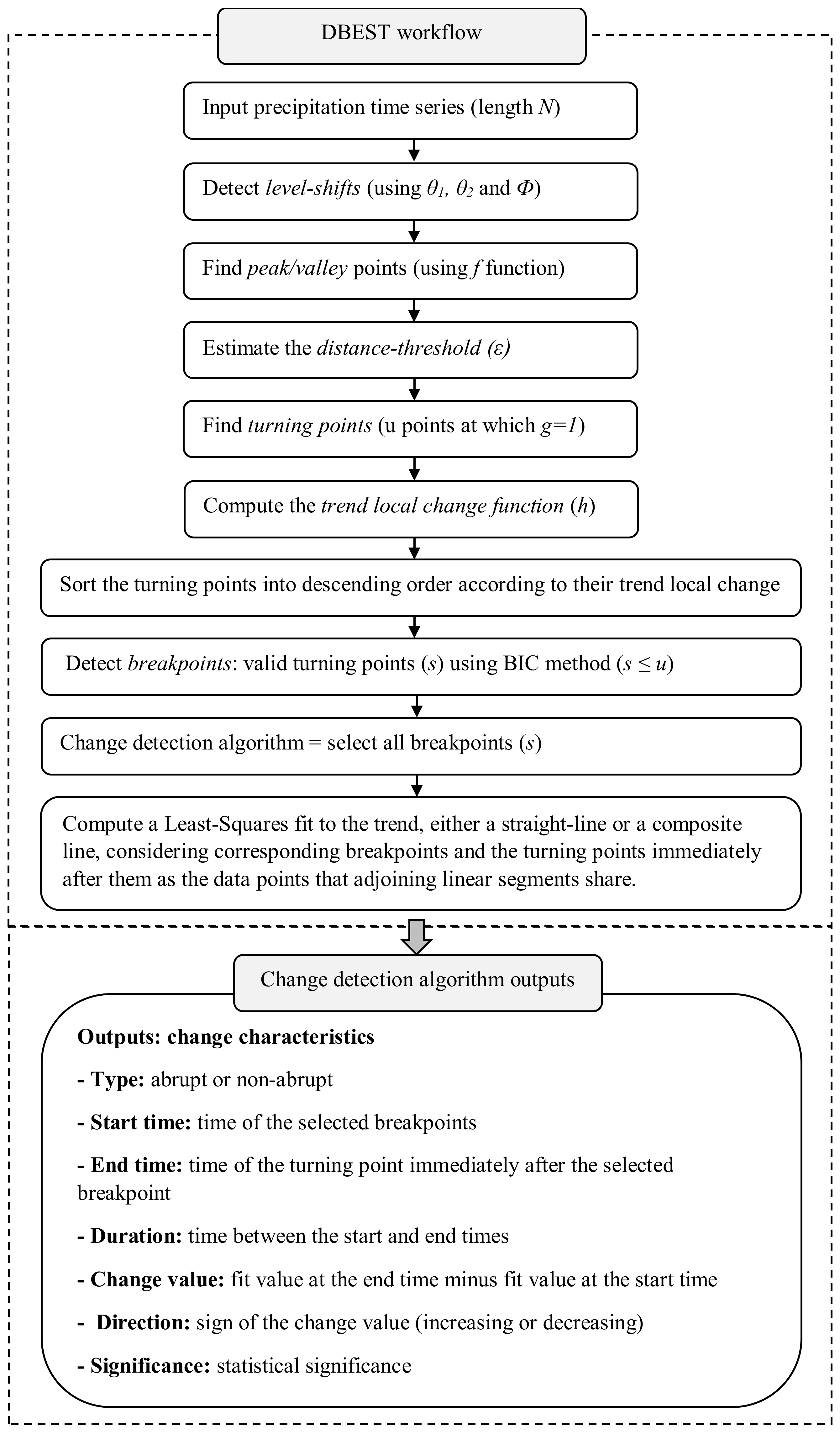
| Threshold | Description |
|---|---|
| First level-shift-threshold (θ1) | The lowest absolute difference in input data (precipitation) between the level-shift point and next datapoint |
| Duration-threshold (ϕ) | The lowest period (time steps) within which the shift in the mean of the data level, before and after the level-shift point, persists, and the lowest spacing (time steps) between successive level-shift points. |
| Second level-shift-threshold (θ2) | The lowest absolute difference in the means of the data calculated over period ϕ before and after the level-shift point |
| Change number (m) | Number of greatest breakpoints of interest for detection |
| Statistical significance level (α) | The statistical significance level used for testing the significance of detected changes |
| Continent | Asia | Africa | Europe | N. America | S. America | Australia | Oceania | |||||||
|---|---|---|---|---|---|---|---|---|---|---|---|---|---|---|
| Year | Neg. | Pos. | Neg. | Pos. | Neg. | Pos. | Neg. | Pos. | Neg. | Pos. | Neg. | Pos. | Neg. | Pos. |
| 1998 | 7.1 | 0.8 | 3.5 | 2.5 | 0.0 | 1.1 | 20.5 | 0.2 | 6.0 | 5.1 | 0.1 | 2.0 | 13.8 | 9.2 |
| 1999 | 1.3 | 1.1 | 6.2 | 1.7 | 1.6 | 0.4 | 0.6 | 0.2 | 2.4 | 1.5 | 1.8 | 2.3 | 4.6 | 3.1 |
| 2000 | 0.9 | 3.4 | 1.8 | 1.1 | 0.4 | 2.6 | 0.9 | 1.6 | 4.0 | 1.3 | 8.9 | 0.0 | 13.8 | 0.0 |
| 2001 | 0.4 | 5.3 | 1.3 | 3.3 | 8.1 | 3.2 | 2.6 | 2.5 | 2.7 | 0.8 | 18.5 | 0.0 | 0.0 | 0.0 |
| 2002 | 1.3 | 5.3 | 1.2 | 2.8 | 9.8 | 0.7 | 0.6 | 3.5 | 4.8 | 1.7 | 0.0 | 0.3 | 0.0 | 0.0 |
| 2003 | 4.2 | 0.3 | 1.6 | 5.2 | 0.0 | 5.1 | 0.1 | 7.1 | 0.4 | 1.9 | 0.0 | 0.1 | 0.0 | 1.5 |
| 2004 | 1.7 | 2.7 | 2.3 | 4.5 | 3.0 | 0.0 | 2.9 | 2.6 | 0.4 | 0.4 | 0.4 | 0.0 | 6.2 | 0.0 |
| 2005 | 2.8 | 1.3 | 2.1 | 3.2 | 1.2 | 6.0 | 7.4 | 2.0 | 0.2 | 3.5 | 1.3 | 3.6 | 0.0 | 1.5 |
| 2006 | 0.9 | 1.7 | 4.3 | 0.8 | 0.7 | 0.0 | 1.8 | 5.1 | 2.2 | 0.4 | 1.3 | 1.3 | 1.5 | 0.0 |
| 2007 | 2.3 | 1.0 | 3.3 | 3.9 | 0.0 | 0.2 | 1.2 | 1.8 | 1.7 | 1.8 | 0.1 | 1.2 | 0.0 | 0.0 |
| 2008 | 1.4 | 4.1 | 3.4 | 2.4 | 0.0 | 1.8 | 1.9 | 0.4 | 5.6 | 1.2 | 0.0 | 0.5 | 3.1 | 0.0 |
| 2009 | 1.2 | 4.5 | 2.8 | 1.6 | 0.5 | 0.9 | 1.9 | 3.1 | 8.1 | 8.4 | 0.1 | 37.4 | 0.0 | 1.5 |
| 2010 | 2.5 | 1.5 | 3.2 | 2.4 | 30.4 | 0.0 | 3.2 | 1.9 | 0.4 | 2.5 | 1.6 | 2.9 | 9.2 | 1.5 |
| 2011 | 0.8 | 3.0 | 1.1 | 4.7 | 0.4 | 3.3 | 5.8 | 1.0 | 4.6 | 1.6 | 11.1 | 0.0 | 15.4 | 0.0 |
| 2012 | 2.4 | 3.4 | 3.8 | 0.7 | 1.8 | 1.6 | 1.3 | 5.0 | 3.0 | 1.3 | 0.6 | 0.1 | 1.5 | 0.0 |
| 2013 | 2.7 | 3.2 | 1.3 | 2.6 | 0.2 | 0.2 | 0.1 | 2.3 | 1.9 | 2.3 | 0.0 | 1.3 | 1.5 | 0.0 |
| 2014 | 0.9 | 3.5 | 4.4 | 3.0 | 1.6 | 0.2 | 0.2 | 2.2 | 4.1 | 1.4 | 0.0 | 0.0 | 3.1 | 1.5 |
| 2015 | 1.8 | 2.9 | 1.7 | 0.7 | 0.0 | 4.2 | 0.8 | 0.7 | 1.3 | 3.1 | 0.0 | 0.0 | 0.0 | 0.0 |
| 2016 | 5.1 | 0.6 | 0.5 | 1.3 | 2.3 | 0.0 | 1.9 | 0.3 | 0.4 | 3.3 | 0.7 | 0.1 | 0.0 | 3.1 |
| 2017 | 0.3 | 8.8 | 0.2 | 1.7 | 0.0 | 7.0 | 0.4 | 0.3 | 1.2 | 0.8 | 0.4 | 0.0 | 0.0 | 3.1 |
| Total | 41.7 | 58.3 | 50.0 | 50.0 | 61.8 | 38.2 | 56.2 | 43.8 | 55.5 | 44.5 | 46.9 | 53.1 | 73.8 | 26.2 |
| Average | 2.1 | 2.9 | 2.5 | 2.5 | 3.1 | 1.9 | 2.8 | 2.2 | 2.8 | 2.2 | 2.3 | 2.7 | 3.7 | 1.3 |
| Climate | Arid (%) | Equatorial (%) | Polar (%) | Snow (%) | Warm Temperate (%) | |||||
|---|---|---|---|---|---|---|---|---|---|---|
| Year | Neg. | Pos. | Neg. | Pos. | Neg. | Pos. | Neg. | Pos. | Neg. | Pos. |
| 1998 | 5.9 | 1.5 | 1.6 | 6.0 | 3.6 | 1.8 | 18.1 | 0.5 | 7.8 | 0.8 |
| 1999 | 3.5 | 1.5 | 2.5 | 1.4 | 2.1 | 0.6 | 1.7 | 0.2 | 2.4 | 1.0 |
| 2000 | 1.6 | 1.9 | 4.7 | 0.9 | 2.3 | 0.9 | 2.2 | 2.2 | 2.4 | 3.8 |
| 2001 | 2.1 | 3.6 | 3.0 | 1.4 | 0.9 | 2.2 | 4.3 | 5.6 | 2.2 | 3.8 |
| 2002 | 1.0 | 3.5 | 2.0 | 2.7 | 3.5 | 4.8 | 1.4 | 3.2 | 5.5 | 3.7 |
| 2003 | 2.8 | 3.3 | 0.5 | 1.2 | 0.8 | 0.4 | 1.3 | 2.0 | 0.9 | 2.6 |
| 2004 | 1.9 | 3.5 | 1.0 | 1.9 | 0.3 | 2.4 | 1.7 | 2.8 | 3.3 | 0.2 |
| 2005 | 2.7 | 1.9 | 0.8 | 6.5 | 7.7 | 1.0 | 2.2 | 1.0 | 2.8 | 2.7 |
| 2006 | 2.7 | 1.1 | 1.1 | 0.9 | 0.8 | 4.3 | 1.0 | 3.6 | 1.7 | 2.5 |
| 2007 | 2.4 | 2.4 | 4.4 | 1.6 | 2.1 | 2.9 | 0.6 | 1.8 | 1.0 | 1.1 |
| 2008 | 2.0 | 2.7 | 3.9 | 0.8 | 3.9 | 3.1 | 0.7 | 3.6 | 4.7 | 3.8 |
| 2009 | 1.9 | 5.5 | 6.4 | 10.5 | 1.6 | 5.4 | 1.3 | 1.2 | 1.2 | 4.6 |
| 2010 | 2.6 | 1.8 | 1.9 | 2.9 | 4.2 | 2.4 | 3.3 | 2.3 | 8.4 | 2.3 |
| 2011 | 1.9 | 3.4 | 4.4 | 1.8 | 2.8 | 1.1 | 3.9 | 2.3 | 1.9 | 2.2 |
| 2012 | 2.7 | 2.4 | 1.8 | 0.7 | 2.4 | 0.9 | 1.7 | 4.8 | 3.5 | 0.7 |
| 2013 | 1.6 | 3.0 | 2.8 | 0.6 | 4.3 | 2.6 | 2.0 | 2.3 | 0.7 | 1.5 |
| 2014 | 2.4 | 3.5 | 3.2 | 1.1 | 5.3 | 1.8 | 0.3 | 0.8 | 0.7 | 0.6 |
| 2015 | 1.6 | 1.7 | 1.3 | 5.4 | 3.8 | 4.3 | 0.4 | 1.3 | 1.1 | 1.5 |
| 2016 | 2.4 | 0.7 | 0.2 | 2.8 | 1.5 | 1.5 | 7.5 | 0.5 | 2.2 | 1.4 |
| 2017 | 0.3 | 5.1 | 0.6 | 0.9 | 1.0 | 0.6 | 0.3 | 3.2 | 0.5 | 4.4 |
| Total | 46.0 | 54.0 | 48.1 | 51.9 | 54.9 | 45.1 | 55.4 | 44.7 | 55.0 | 45.1 |
| Average | 2.3 | 2.7 | 2.4 | 2.6 | 2.7 | 2.3 | 2.8 | 2.2 | 2.7 | 2.3 |
| Climate | Arid | Equatorial | Polar | Snow | Warm Temperate | |||||
|---|---|---|---|---|---|---|---|---|---|---|
| Change (mm) | Pos. | Neg. | Pos. | Neg. | Pos. | Neg. | Pos. | Neg. | Pos. | Neg. |
| Mean | 164.0 | −174.3 | 874.4 | −846.8 | 194.2 | −159.5 | 326.4 | −323.7 | 574.5 | −634.3 |
| Max | 2719.6 | −2.9 | 3122.1 | −223.0 | 1074.2 | −57.4 | 981.9 | −98.6 | 4967.6 | −126.9 |
| Min | 3.2 | −2113.6 | 198.0 | −2998.4 | 57.7 | −1348.0 | 88.9 | −1547.0 | 116.5 | −2801.8 |
Publisher’s Note: MDPI stays neutral with regard to jurisdictional claims in published maps and institutional affiliations. |
© 2022 by the authors. Licensee MDPI, Basel, Switzerland. This article is an open access article distributed under the terms and conditions of the Creative Commons Attribution (CC BY) license (https://creativecommons.org/licenses/by/4.0/).
Share and Cite
Kazemzadeh, M.; Hashemi, H.; Jamali, S.; Uvo, C.B.; Berndtsson, R.; Huffman, G.J. Detecting the Greatest Changes in Global Satellite-Based Precipitation Observations. Remote Sens. 2022, 14, 5433. https://0-doi-org.brum.beds.ac.uk/10.3390/rs14215433
Kazemzadeh M, Hashemi H, Jamali S, Uvo CB, Berndtsson R, Huffman GJ. Detecting the Greatest Changes in Global Satellite-Based Precipitation Observations. Remote Sensing. 2022; 14(21):5433. https://0-doi-org.brum.beds.ac.uk/10.3390/rs14215433
Chicago/Turabian StyleKazemzadeh, Majid, Hossein Hashemi, Sadegh Jamali, Cintia B. Uvo, Ronny Berndtsson, and George J. Huffman. 2022. "Detecting the Greatest Changes in Global Satellite-Based Precipitation Observations" Remote Sensing 14, no. 21: 5433. https://0-doi-org.brum.beds.ac.uk/10.3390/rs14215433