Article

VirtuaLot—A Case Study on Combining UAS Imagery and Terrestrial Video with Photogrammetry and Deep Learning to Track Vehicle Movement in Parking Lots

1
Conrad Blucher Institute for Surveying Science, Texas A&M University-Corpus Christi, Corpus Christi, TX 78414, USA
2
Department of Computing Sciences, College of Engineering, Texas A&M University-Corpus Christi, Corpus Christi, TX 78414, USA
3
Innovation in Computing Research Lab, Texas A&M University-Corpus Christi, Corpus Christi, TX 78414, USA
*
Author to whom correspondence should be addressed.
Remote Sens. 2022, 14(21), 5451; https://0-doi-org.brum.beds.ac.uk/10.3390/rs14215451
Submission received: 17 August 2022 / Revised: 17 October 2022 / Accepted: 24 October 2022 / Published: 29 October 2022
(This article belongs to the Special Issue Urban Sensing Methods and Technologies)

Abstract

:
This study investigates the feasibility of applying monoplotting to video data from a security camera and image data from an uncrewed aircraft system (UAS) survey to create a mapping product which overlays traffic flow in a university parking lot onto an aerial orthomosaic. The framework, titled VirtuaLot, employs a previously defined computer-vision pipeline which leverages Darknet for vehicle detection and tests the performance of various object tracking algorithms. Algorithmic object tracking is sensitive to occlusion, and monoplotting is applied in a novel way to efficiently extract occluding features from the video using a digital surface model (DSM) derived from the UAS survey. The security camera is also a low fidelity model not intended for photogrammetry with unstable interior parameters. As monoplotting relies on static camera parameters, this creates a challenging environment for testing its effectiveness. Preliminary results indicate that it is possible to manually monoplot between aerial and perspective views with high degrees of transition tilt, achieving coordinate transformations between viewpoints within one deviation of vehicle short and long axis measurements throughout 70.5% and 99.6% of the study area, respectively. Attempted automation of monoplotting on video was met with limited success, though this study offers insight as to why and directions for future work on the subject.

1. Introduction

In many photogrammetry applications, the knowledge of a camera’s combined position and orientation, also called camera pose, is essential even if that camera remains fixed in a static position [1,2]. Static camera pose can be measured via hardware using external surveying instruments, while mobile cameras can use onboard positioning systems such as inertial measurement units (IMUs) and/or global navigation system satellite (GNSS) receivers [3,4,5,6,7,8,9,10,11]. There are numerous studies on the subject of computing mobile camera pose relatively without positioning hardware from one camera frame to the next to create point clouds, which can be georeferenced using known position targets in images, called extracting “structure-from-motion” (SfM) [8,12,13,14]. Additionally, SfM can be coupled with hardware positioning equipment in a real-time process that forms the basis of simultaneous localization and mapping (SLAM) of an environment [15,16,17,18,19].
Computation of point cloud products using computer vision typically relies on keypointing algorithms [12,20]. These algorithms automatically detect and identify salient points in images which can be subsequently identified again up to a certain degree of change relative to the initial perspective [21,22,23,24,25,26,27,28]. Through application of geometric principles and probabilistic statistics, coordinate points located in two images can be used to simultaneously determine 3D point locations in space for 2D points in both images and derive relative camera positions for the images. Iterating this process over various combinations of image pairs can lead to accurate estimations of camera pose, and relative point coordinates in 3D space, the necessary components for creating point clouds [12,14,29,30]. More recently, some deep learning approaches to pose estimation have also been developed, a large number being derived from Kendall et al. [31]. However, the input data used with these methods is somewhat uniform with regard to certain meta-characteristics [31,32,33]. For example, when computing a point cloud using tourism photographs, SfM is capable of identifying two camera positions which could be completely opposite to each other as long as there is some coverage of the same area by other images in positions that somewhat interpolate the transition between the original two camera poses [20,34,35,36]. These images are generally of a perspective which would include a horizon line, mirroring the positions in which a human would observe a scene. Alternatively, aerial imagery observing nadir may be used in an identical pipeline to create point clouds of structures and terrain over wide areas [3,12,13].
For quite some time, mixing both aerial and terrestrial imagery during SfM processing was only possible in an automated fashion if there were enough images captured between nadir and terrestrial perspective shifts that keypointing could be used to track camera pose changes effectively unless other positioning systems could be relied upon to accurately record camera pose and register it in post processing [3,35,36,37,38]. In a certain sense, an SfM generated point cloud, often called a sparse point cloud, can be described as a database of 3D points which have known point descriptors attached to them from various perspectives. Each image processed by an SfM pipeline will extend the existing point description records while also adding new points. Some advanced keypointing techniques have been developed to address the problem of high transition-tilt, allowing registration between images with signifcant changes to camera pose, but their additional complexity is of variable effectiveness and incurs additional processing overhead [20,34,35,36]. Some deep learning approaches have also addressed image keypointing, image registration, and similar topics, but they are similarly constrained in that they require the same data as an SfM pipeline to be able to effectively determine an input camera’s pose reliably after a lengthy training phase [31].
However, there exists a sibling process to stereo-photogrammetry, which itself is derived from the principles of stereo-plotting, called “monoplotting” [39,40]. Monoplotting appears to have been primarily used in manual applications for digitizing perspective imagery data and converting it to an aerial perspective, using manually matched point coordinates between perspective and aerial images accompanied by digital surface model (DSM) data [40]. Examples of monoplotting applications include using historical imagery to map vegetation change onto thematic maps and using perspective imagery to demonstrate how the elevation and flow of Arctic ice has changed over a long period of time [40,41].
The primary objective of this case study is to develop a framework to record vehicles as they move throughout a parking lot monitored by existing surveillance equipment (terrestrial video camera) already installed on a university campus, presented in a format which allows for general understanding of the movement of vehicles across the area and is not impacted by the equipment’s pan-tilt-zoom functionality. This study evaluates the impact of monoplotting as an additional automated layer of relatively rapid camera pose estimation over the classic computer vision problem of detecting and tracking vehicles via terrestrial video, similarly to the pedestrian tracking method applied by Petrasova et al. [42], and trajectory estimation techniques applied by Chen et al. [43]. Aside from our earlier study [44], which forms the basis for this extended paper, there are some studies which cover similar and related topics, including continuous camera localization as proposed by Jiang et al. [45], and similar approaches to camera pose processing and integration as presented by Zhang et al. [46], Han et al. [47], and Luo et al. [48]. A distinct difference between those studies and this one is that either prior camera position and object information is available as in Zhang et al. [46], or camera calibration data is available as in the others [45,47,48]. While the target camera pose data is available in this study, in contrast to the other studies this data is used for validation purposes only and not provided as a starting point for monoplotting (which it could be) in order to evaluate the proposed methods independently.
This work also engages various fields of computer vision, specifically neural network based object detection and algorithmic object tracking techniques. However, an in-depth review of these methods is better served by the following references: [7,48,49,50,51,52,53,54,55,56,57,58,59,60,61,62,63]. The quality of the monoplotting solutions can be affected by several factors present in this study. Specifically, the physical components of the camera itself should be quite inviolate to change, but the weatherproof chassis or the mechanical control mechanisms contained within, may be more affected by varying ambient conditions. These variations can also be exacerbated by changes in the shape of a plexiglass dome cover when it experiences thermal flux [64]. In particular, air temperature and pressure appear cause a degree of dynamic variation in the mechanical tolerances of the camera’s pivot-tilt-zoom functionality, reducing its precision when attempting to return to a calibrated home position. The changes in mechanical tolerances and shape of the plexiglass cover should both be physically minuscule and ordinarily would be considered negligible. However, monoplotting requires a calibrated camera image with a known static pose, and even small deviations when returning to a set home position will have impacts on coordinate transformation accuracy as distance from the camera increases. Such deviations, especially deviation when adjusting focal length for optical zoom, can render previously recorded calibration data invalid over the course of a day or when the weather changes. Furthermore, while the camera position can be externally measured, the camera also provides an API which defines its own coordinate space. Meaning there is also the potential for additional precision error when converting from camera space to world space.
In summary, this study develops a computer vision and object tracking pipeline, and explores the feasibility of leveraging monoplotting, to create an accurate, real-time visualization of parking lot vehicle traffic overlaid on an aerial map (i.e., orthomosaic image) with a terrestrial video camera whose geometric calibration and pose changes unpredictably. The entire framework is named VirtuaLot. With this motivation in mind, the contributions of this paper are as follows:
  • A computer vision pipeline which can detect and track vehicles that enter and exit a parking lot, using an available deep learning object detection network and traditional image processing techniques to improve the pipeline efficiency by reducing and constraining inputs and outputs to both deep learning object detection and more traditional tracking algorithms.
  • Using monoplotting as a mechanism to automate the definition of tall, vertically occluding objects in a perspective camera image.
  • An investigation into the effects of using a camera with unpredictably changing internal geometry as input for the monoplotting process, to evaluate its suitability as a mechanism for registering perspective video and uncrewed aircraft system (UAS) aerial imagery. Attention is also paid to challenges encountered while attempting to automate the monoplotting process using various keypoint descriptors.
The remainder of this paper is structured accordingly: Section 2 details the information necessary to accomplish monoplotting atop the proposed computer vision pipeline, as well as the specific details of the study area and datasets collected and used in this study. The methodology outlined in Section 3 introduces the data preparation steps alongside definition of the computer vision pipeline and the effects of direct image registration via monoplotting, as well as the implementation of automatic occlusion detection. It also investigates adaptations explored to overcome challenges with automating monoplotting between the two views of the study area. Section 4 is arranged in alignment with the methodology section, starting with review of coordinate transformation accuracy in single image monoplotting, then quantitative analysis of the computer vision pipeline, followed by measuring the accuracy of the feature matching results and the effectiveness of the occlusion handling process, ending with analysis of the impact of the effects of single and sequential image monoplotting. Section 5 reviews the general efficacy of the results in the proposed context of the research as a whole. Finally, Section 6 concludes this work and discusses potential future development.

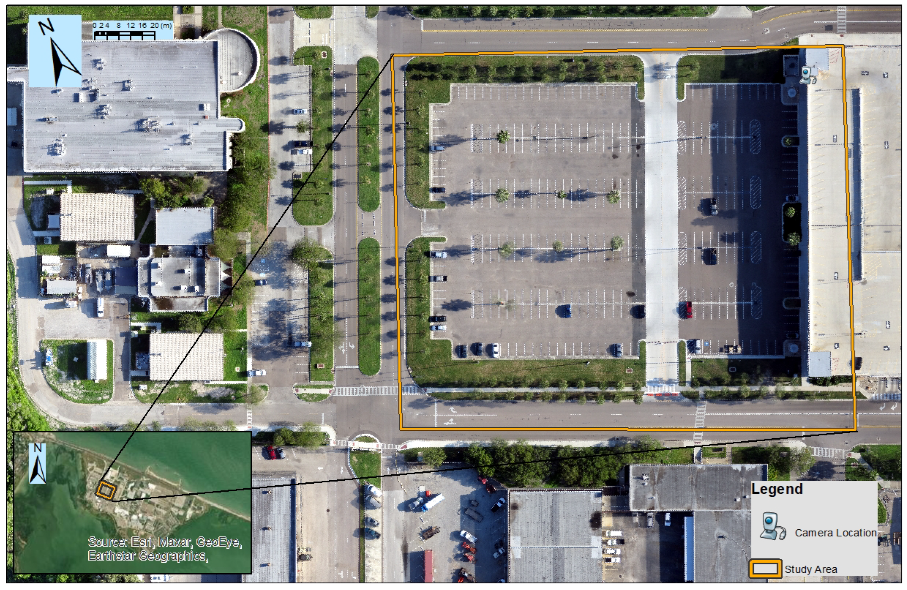
2. Study Area and Datasets

The study area is a parking lot located near the center of the Texas A&M University Corpus Christi (TAMUCC) campus in Corpus Christi, USA, approximately 93 m wide by 118 m long, highlighted in orange on Figure 1. While not strictly necessary for purposes of the application, for this case study a ground survey was performed to measure the position of the perspective security camera as closely as possible using a total station and known Continuously Operating Reference Station (CORS) benchmarks located on the campus grounds to determine the position (but not orientation) of the camera housing in world space to a high degree of precision. An average position for the camera was calculated by taking four measurements targeting the edges of its circular chassis mount, equidistant around its perimeter.
The datasets in this case study are split into two categories: perspective video files provided by the TAMUCC Police Department, and UAS imagery products that were generated from a small UAS flight conducted by the TAMUCC Measurement Analytics Lab (MANTIS). The UAS flight collected 1565 georeferenced photos, which were post-processed using Pix4D Mapper to generate an aerial orthomosaic image and digital surface model (DSM) of the campus area. The target parking lot for study and its surrounding area of interest were extracted from the larger campus flight to reduce image sizes to workable levels in this application.
An example of the perspective view from the video camera dataset is shown in Figure 2. Normally, a calibration pattern would also be used to correct camera lens distortion for this perspective video camera. However, attempts to calculate a valid camera calibration over the course of the study would yield different results. As best we can determine, changes in static air pressure, temperature, and humidity cause the weatherproof housing media and control mechanisms to expand and contract over time, as well as during and after changes in weather conditions. This is not typically an issue affecting the camera component of the actively cooled AXIS Q6044-E PTZ, but it does affect the weatherproof cover and the pan-tilt-zoom mechanisms.
The thermal expansion of the polycarbonate weather housing is quite low, 0.065 mm/m °C as per [64]. To put this into context, a 15 °C change in a 10 cm polycarbonate part can cause thermal expansion of ±1 mm [65]. This is an extremely small value—for a flat part. However, for a dome shape, such as the weatherproof housing, considering the degree of temperature difference on a typical Texas summer day (a conservative estimate being from 20 to 38 °C, not accounting for inclement weather which can get as cold as 10 °C if not lower for periods of time), the weatherproof housing can elongate or contract in size as well as expand or shrink in thickness over time, changing the exit position and travel distance for light rays passing through the housing relative to the camera origin. This also assumes a perfect, uniform thickness dome covering an imperfection free lens, neither of which exist in this scenario. Because of this, a lens calibration taken in the morning hours using a checkerboard pattern will not be the same as a calibration taken in the middle or hottest parts of the day even if the camera is not manipulated. Additionally, the gearing of the camera mechanisms may be subject to similar thermal effects, and the precision of the “return to home position” function also varies over the course of a day. These are not instantaneous issues, but rather ones that proceed from collecting data over time as environmental flux causes these effects. In combination with the need to allow for ad hoc camera movement, the imprecise “return to home” function can invalidate any fixed configuration position, and imprecise “return to original zoom” mechanisms can invalidate any recorded calibration. With this in mind, the study forgoes any notion of calibration for the perspective video data, instead analyzing the raw data and how much error the uncalibrated perspective view introduces into the end solution.
There are two perspective video samples chosen for discussion in this application study: both recorded at 30 frames per second (FPS) in early December 2016 and September 2017. One sample is a four hour window with some interesting dynamic motion of low numbers of vehicles, and the other is one of a full parking lot with high numbers of vehicles moving through it at any given time. The first sample is presented as the vehicles which are present are ones which demonstrate challenging instances of detection and tracking to follow, as a representation of the capabilities of the application. The second sample tests the accuracy and performance of the application handling high numbers of vehicles moving in common traffic patterns. The first sample was reduced from 432,000 frames to 6646 frames total by eliminating long periods of inactivity from analysis, resulting in a three and a half minute sample with 46 vehicles annotated. The second sample is used as recorded, with 200 vehicles annotated over a two and a half minute time period in a very full parking lot, roughly three new vehicles every two seconds. Vehicle detection and tracking data was annotated from the video samples using a supervised image processing workflow, combining background subtraction and the minimum bounds of contour detection with a linear regression function to validate the size of a moving object as appropriate relative to its position in the video frame. A centroid tracker could very reliably track these “detections”, allowing mostly automated annotation of the perspective video samples with some manual review to create ground truth datasets for measuring object detection and tracking performance. This annotation method was impressively accurate, though non-trivial to set up and not robust to changes in camera position.
Aerial imagery from the MANTIS Lab was collected using an eBee fixed wing UAS platform equipped with a 20 MP SenseFly SODA red–green-blue (RGB) digital camera with a 10.6 mm lens mounted in a nadir observing orientation recording an average 2.78 cm ground sample distance (GSD) from an average height of 91 m above ground level. Onboard GNSS image positions were recorded in WGS84 coordinate reference system (CRS). Although the survey targeted low wind conditions, there are small changes in orientation and tilt of the camera throughout the flight due to effects of wind and flight dynamics. As such, the data collected does not represent a true nadir-perspective image set. It should also be mentioned that the UAS flight surveyed the entire TAMUCC Ward Island campus (1.32 km2), making it conducive for utilization of a fixed wing platform. Therefore, the study area represents only a small portion of the entire region mapped.
A ground control network was established using the “NAD 1983 State Plane Texas South FIPS 4205—Feet” CRS with the GRS80 ellipsoid, and nine ground control points surveyed in over a 1.32 km2 survey area to improve the accuracy of the point-cloud derived products. All positioning data was converted to the NAVD88 vertical datum from Geoid12B referencing the Texas Department of Transportation real-time network (RTN) for control measurements. During reconstruction processing and adjustment, the ground control point network covering the flight area reported a vertical RMSE of 0.9 cm. However, of greater concern in this application is the vertical accuracy of the DSM, particularly its representation of the ground surface, as a high quality DSM is critical for accurate monoplotting computation. Fortunately, in this aerial survey, the vertical deviation of the ground plane of the parking lot as represented by the DSM is expected to be in the range of 2–4 cm, or less. This estimation is based on the vertical accuracy of the point cloud used to interpolate the DSM measured relative to the control network and over flat surfaces in the survey area.
The specifications of the platform sensors, raw images, orthomosaic derived from overlapping raw images, and DSM derived from the same set of overlapping UAS images using SfM photogrammetry are outlined in Table 1. The DSM is necessary for the computation of the formulae described in Section 3.2 and implementation of methods in Section 3.3. Note that the nature of the project only requires a partial overlap between perspective and aerial viewpoints, and it was fortunate that the perspective camera field of view shown in Figure 2 was entirely contained within the aerial orthoimage, but it is not strictly necessary. Additionally, note that while an aerial orthoimage and DSM are used in this study, it is possible to replace them with normally collected, calibrated aerial imagery and a DSM collected by a LiDAR system for functionally the same inputs.
In regards to training data for the neural network, the data for the bus, car, and motorbike classes was extracted from the PASCAL VOC 2012 dataset: out of the 20 classes and 16,682 samples available, there were 421 bus samples, 1161 car samples, and 526 motorbike samples, totaling 2108 positive class samples. The remaining samples of other classes were completely eschewed to avoid additional complexity that may arise from being able to detect them. There are also several pre-processing steps necessary to implement the application study, some derived from each dataset individually and others requiring multiple datasets being analyzed in tandem, which are discussed in the Methods section.

3. Methods

The collection of methods employed in developing the VirtuaLot framework proposed in this case study consists of two parts, the computer vision pipeline and the extension of that pipeline using monoplotting to calculate coordinate transformations between the two image perspectives. The computer vision pipeline outlined in Section 3.1 is the core engine of this application study, but the objective of the research is to leverage it in an experimental way by automating the monoplotting component (Section 3.4) to estimate occlusion regions in the perspective view (Section 3.3), and to investigate any effects or artifacts that arise during the process. A flowchart of the methods implemented for the VirtuaLot framework is outlined in Figure 3.

3.1. Computer Vision Pipeline

The computer vision pipeline can be described as a bespoke object detection and tracking solution. Within the scope of this component specifically, the object classes of interest are constrained to those commonly found in a parking lot, primarily vehicles, such as cars, pickup trucks, and motorbikes, discounting larger trucks or delivery vans. The computer vision pipeline was implemented using the Darknet deep learning framework [66] for initial (and optionally continuous) object detection and tested with some of the object tracking methods available in OpenCV: Kernalized Correlation Filters (KCF) [59], Boosting [67], Track-Learn-Detect (TLD) [55], and MedianFlow [56]. A collection of annotated images is required for training the Darknet framework, or a pre-trained network may be used. The annotated images must be a series of image and text files which describe the classification (category) of an area as well as the number of coordinates which encompass that area, and the actual coordinate locations. A custom Darknet model was trained using a subset of the PASCAL VOC 2007 and 2012 data [68], specifically on the aforementioned object classes at the beginning of this section, to evaluate if training with a reduced dataset would affect the final model compared to training on the full dataset. The training process for the VOC subset model mimics the process for the full VOC model published by Redmon [66], using the same 16,551 training images and 4952 testing images for validation, an approximate 75–25% split. Other object classes available in the dataset were completely eschewed in the subset compared to the full model. Identical training parameters, including the moving learning rate ( 10 3 , 10 2 , 10 3 , 10 4 ), momentum (0.9), and decay rate (0.005) were applied as in the original paper [66], however training was only run for 45 epochs, instead of the original 135, with the learning rate ranges adapted accordingly in an effort to avoid over-fitting on a smaller datatset sample. The smaller subset-trained network provided a very minor performance improvement at the cost of slight detection consistency compared to the fully trained network. Functionally, detection behavior of the two networks was nearly identical. Multiple running options for the computer vision pipeline were developed to investigate the effects of different approaches and methods as applied to the study, allowing a choice of the neural network used to power object detection and a choice of tracking method implementation. Several additional performance affecting options were also developed, including different ways to arrange input tensors passed to the neural network, the size of tracked object area used to initialize detected objects, and a motion sensitive triggering mechanism powered by CPU or GPU background subtraction to reduce the number of calls to the neural network. The effectiveness of each option and its impacts on the computer vision pipeline was determined by parameter sweeping all combinations of possible options. The ground truth annotation algorithm, effectively serving as an additional detection and tracking method, was also evaluated with similar swept parameters to establish performance baselines.

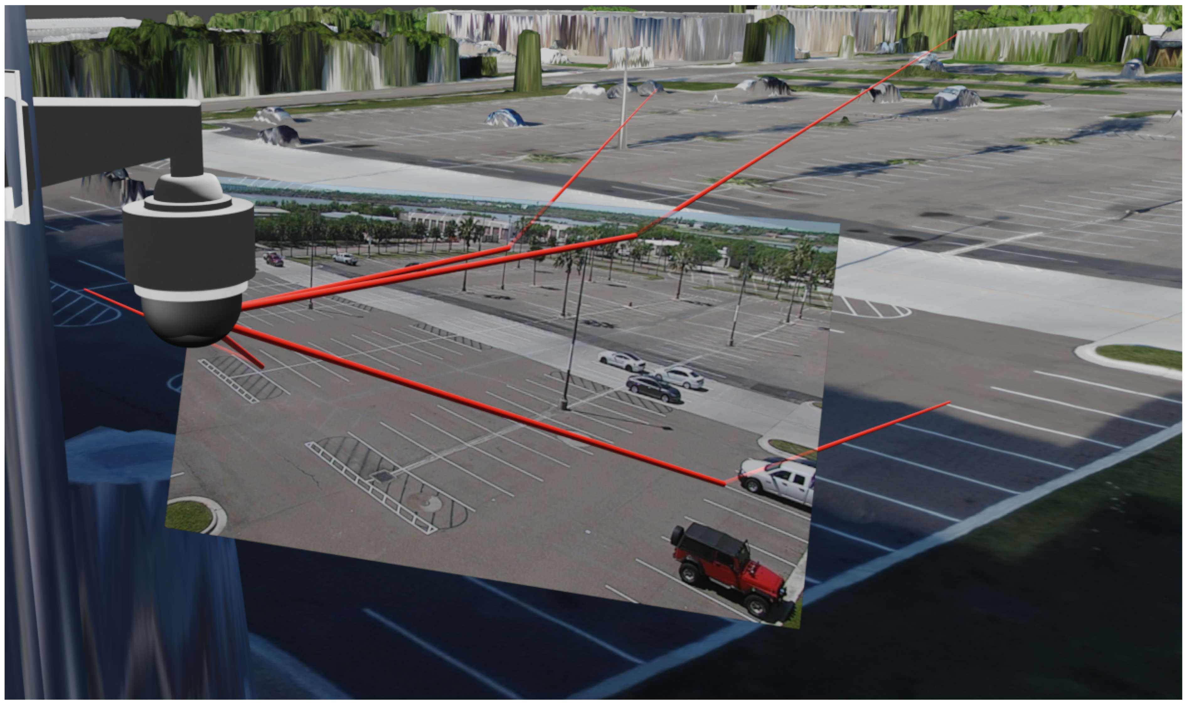
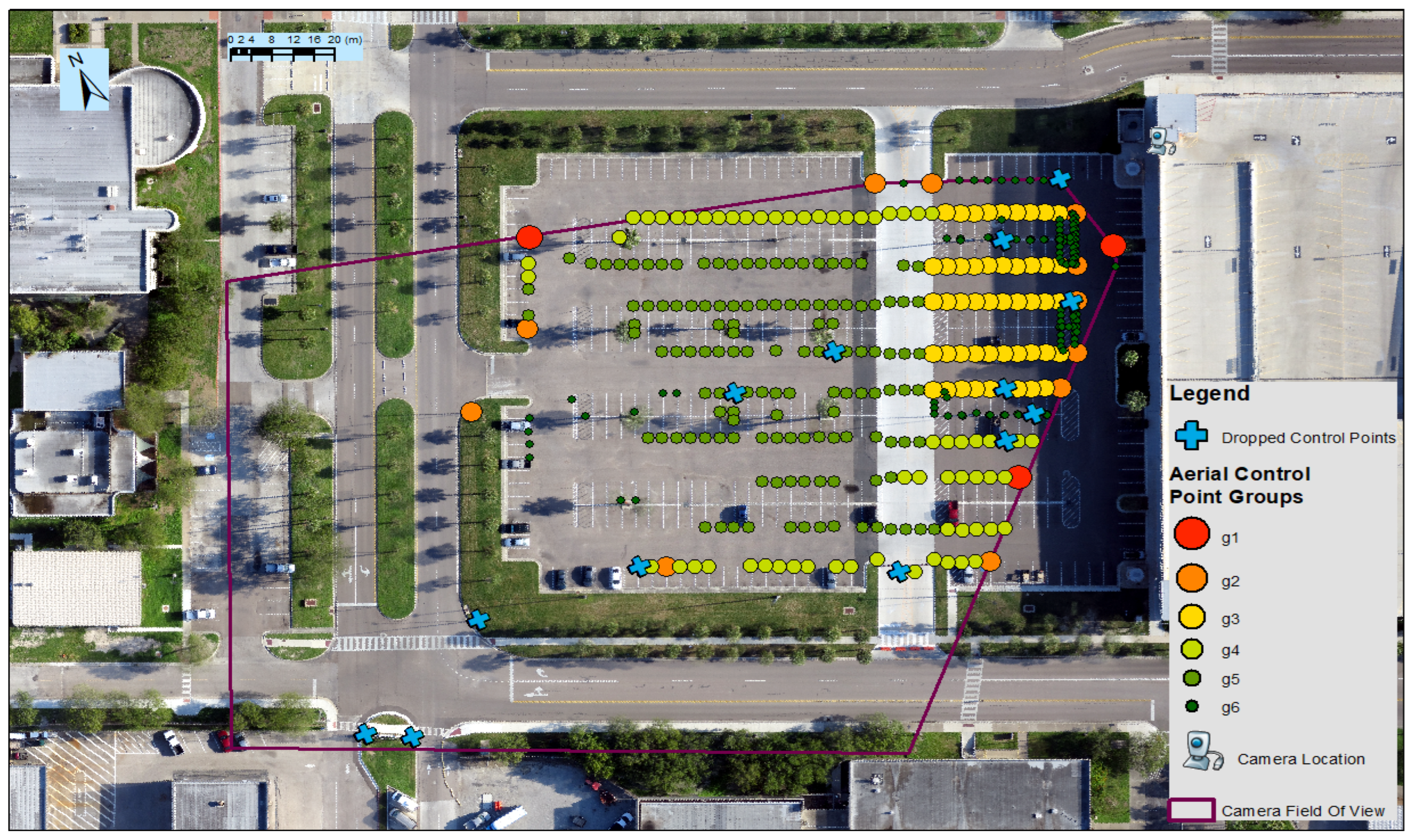
3.2. Single Frame Registration with Monoplotting

Traditional monoplotting normally requires a recorded camera pose and preferably two calibrated camera images, with source positions in three-dimensional space as coordinates X, Y, Z coupled with ω , ϕ , κ describing the camera orientation in terms of roll, pitch, and yaw when an image was taken [39]. A conceptual visualization of monoplotting is shown in Figure 4. However, there are several mathematical relationships which can be leveraged to reconstruct complete or partial pose parameters given a series of known points in a pair of images, usually of the same scene [39]. As monoplotting is usually a fully manual process, the linear form of its collinearity equations can be simplified as Equations (1) and (2):
x a F 0 + v x α = b 11 Δ X a + b 12 Δ Y a + b 13 Δ Z a
y a G 0 + v y α = b 21 Δ X a + b 22 Δ Y a + b 23 Δ Z a
where b n n is shorthand for a series of partial derivatives taken from the functions of rotation angles ( ω , ϕ , κ ) multiplied by coefficients of the orthogonal transformation matrix m between image plane and object space orientation. X a , Y a , Z a are object space coordinates, x a , y a are image space coordinates, and F 0 , G 0 are functions with estimated, iteratively solved values [39].
In this case study, image registration between the perspective terrestrial video sequences and the UAS aerial orthomosaic detailed in Section 2 is performed by first computing an image homography to determine 2D inlier and outlier points, followed by solving for the camera pose using an iterative adjustment computation as outlined in [39]. The elevation values necessary to compute the 2D–3D transition [39] are retrieved from the DSM at the marked coordinate locations in Figure 5 to provide the necessary 2D-3D context. Figure 6 displays the DSM values linked to the selected points shown in Figure 5. To measure the effects of monoplotting on the image registration process, 399 manually annotated point pairs are divided into seven recursively growing subsets, as shown in Figure 5, to simulate variations in keypoint matching efficacy. The 399 points were drawn from a larger set, filtered by computing the intersection of Shi-Tomasi corner detection [27] results and the locations of image keypoints detected with the list of algorithms presented in Section 3.4. The paired points are manually annotated to discard non-ground level features and features which had no temporal overlap between the aerial orthomosaic and the perspective video, for the purpose of measuring the accuracy of coordinate transformations using a well-defined registration between a single video frame and the aerial image, and how the number of keypoints successfully matched can influence the overall accuracy.
The efficacy of registration with each group of an increasing number of points is determined by the deviation present in point transformations between the aerial image and perspective video coordinate systems, an example of which is visualized by Figure 7. We note that the end product of this image registration specifically treats the aerial orthomosaic origin as true and fixed, so that the iterative solution focuses on solving for the perspective camera origin alone.

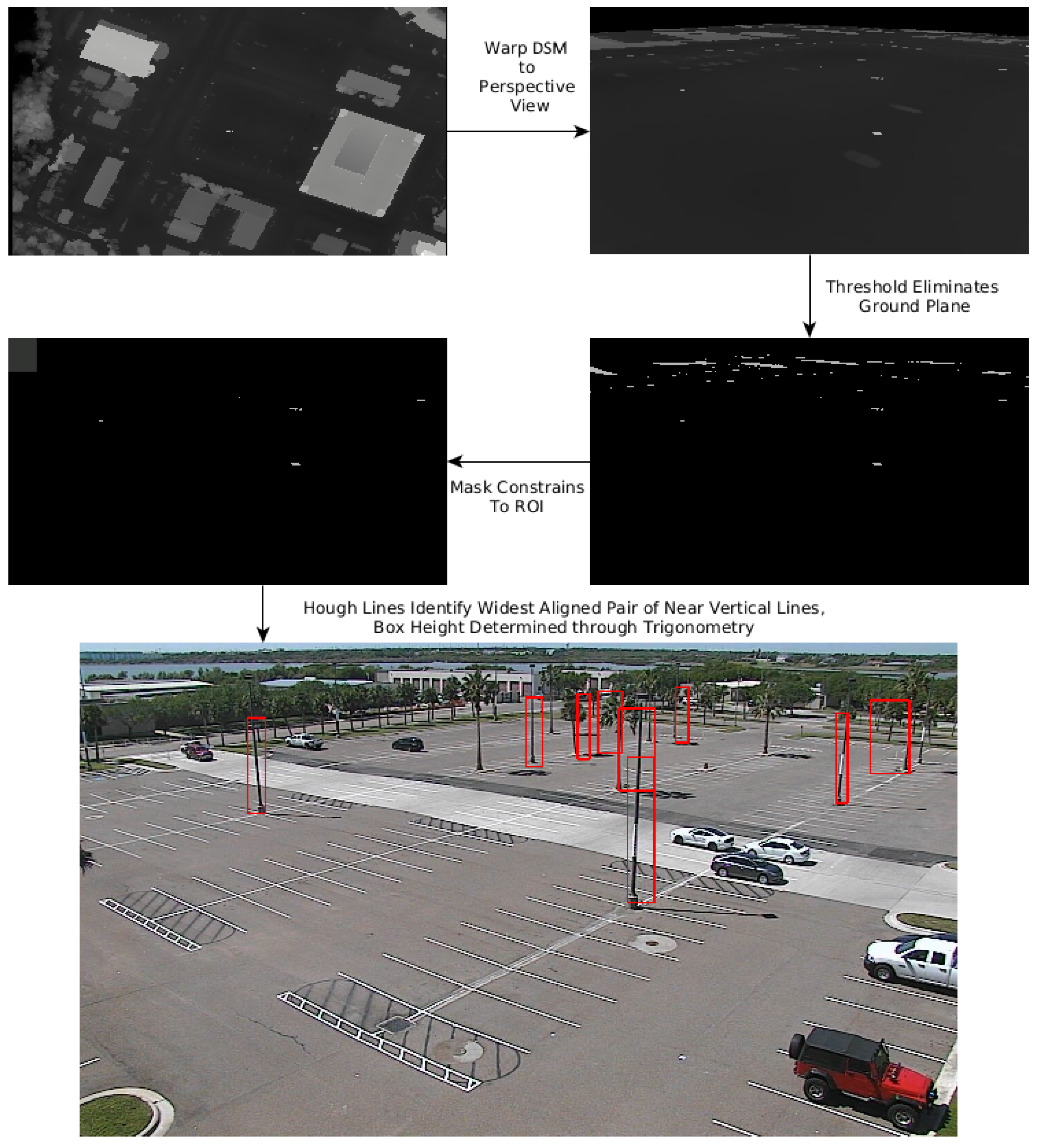
3.3. Automated Occlusion Detection

Using the registration defined by the monoplotting process, it occurs that a potentially viable process for identifying occlusion regions created by static vertical elements in the perspective view, such as trees or streetlights, using the DSM is possible.
By projecting the DSM into the perspective image, an example of which is shown in Figure 6, the intersection of the ground plane and regions of potential occlusion can be identified in the perspective view directly. The DSM can then be masked using the same regions of interest defined in the background subtraction constraint to eliminate extraneous elevation data. Using the width of the transformed elevation feature on the ground, an occlusion region can be initially defined starting from its lowest available coordinate to the top of the image. Analyzing the Hough [69] lines computed in each region, the strongest set of near-to-vertical lines with matching orientations can be used to roughly refine the width of an occlusion region, and the highest horizontal line can be approximately computed from the value of the DSM via trigonometry to cap the occlusion region. These occlusion regions can then inform object tracking methods that the object they are tracking is potentially occluded, allowing for more robust handling of occluded vehicles as they maneuver through the parking lot area.
Figure 6. The process and results of using images registered via monoplotting to determine approximate occlusion areas from a Hough transformation cross referenced with the DSM and trigonometry. Note that some occlusion regions encompass vertically oriented features entirely, while some only encompass partial features. Furthermore, the occlusion regions are substantially buffered in this image for the reader. The actual regions are quite closely constrained to the actual vertical lines in each region.
Remotesensing 14 05451 g006

3.4. Automated Monoplotting

In order to fully automate the process of monoplotting, various keypointing methods available in OpenCV were applied to both the UAS orthomosaic and the perspective video to measure the efficacy of such methods at successfully computing a correct image registration via keypoint matching. Keypoint methods examined include: Scale Invariant Feature Transformation (SIFT) [26], Speeded Up Robust Features (SURF) [25], Oriented Fast and Rotated Brief (ORB) [21], Accelerated-KAZE features (AKAZE) [70], and Binary Robust Invariant Scale keypoints (BRISK) [71]. Both the standard implementation of the aformentioned methods and a version leveraging the affine keypointing process outlined by Yu et al. and Morel et al. are tested [35,36]. Notably, in order to acquire results in a timely manner, the affine method keypoint datasets (titled ASIFT, ASURF, AORB, AAKAZE, and ABRISK) were constrained to using the same number of keypoints that their standard method counterpart computed for each frame, filtered in order of strongest responses first.
After computing keypoint matches between perspective video frames and the UAS orthomosaic, the z-dimension required for computing the 2D-3D monoplotting solution is retrieved from the DSM using the closest available cell value. The monoplotting of each frame was processed two ways. First, using keypoints that were detected across the entirety of the frame. Second, using the same mask defined for isolating the parking lot area used in Section 3.3, to reduce the number of keypoints and concentrate them within the area of interest. The efficacy of monoplotting automation using each keypointing technique is computed through statistical analysis of comparisons to the pose of the camera computed by the single frame iterative process and the ground truth location from the survey.

4. Results

This section first reviews the accuracy of using a single image monoplotting solution to perform coordinate transformation, then moving into light qualitative analysis of the object detection and tracking pipeline performance and how well it integrates with the single image monoplotting solution and vertical occlusion detection. Finally, results on automation of monoplotting close out the section.

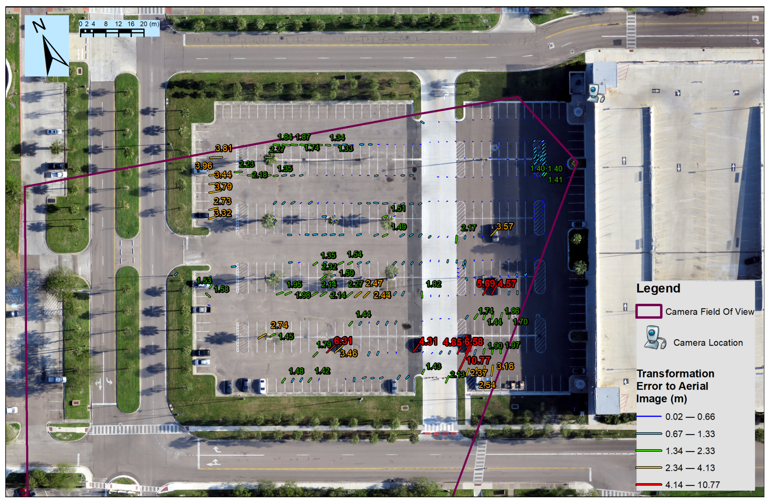
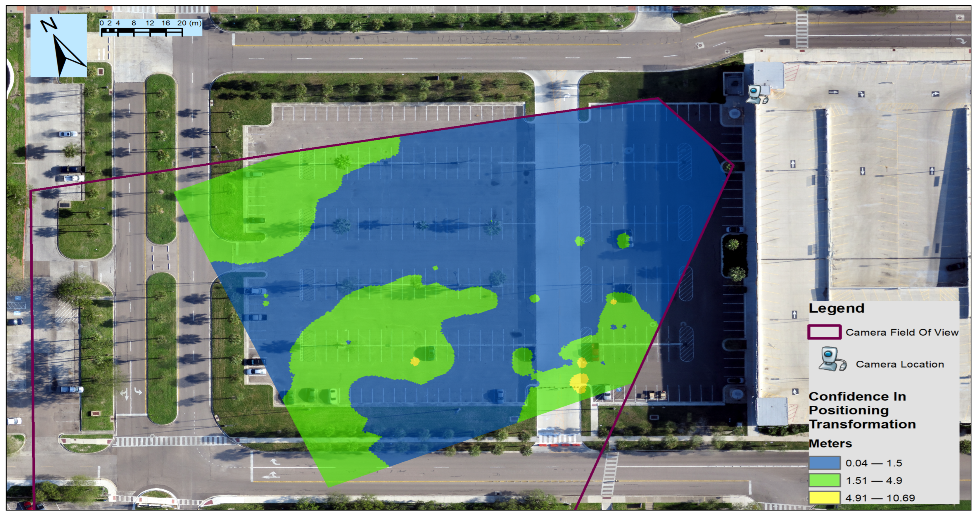
4.1. Single Frame Registration via Monoplotting Results

The effects of ignoring lens calibration are also demonstrated in Figure 7, Figure 8, and Figure 9 where the effects of the transformation show significant distortion near the edges and with increased distance from the camera origin.
Figure 7. The results of using the recursively larger groups of points outlined in Figure 5 to reproject the perspective image into the aerial orthoimage plane. Note the distinct linear deformation in some of the lateral parking space lines as well as variable degrees of alignment to the parking lot borders and the bottom interior row of parking spaces around the edge.
Remotesensing 14 05451 g007
The effects of distortion due to being unable to calibrate for the internal geometry of the perspective camera are visualized in Figure 7 as transformation boundaries of the perspective image into the aerial plane, Figure 8 as discrete measurements, and continuously quantified in Figure 9 and Figure 10.
Figure 9 visualizes the ranges of transformation accuracy for any given pixel between perspective and aerial images in the area of interest under the best possible brute-force solution able to be achieved with manual monoplotting using a single perspective video frame for registration reference. There are two areas of significant pixel deviation in the top-left and bottom-right corners in Figure 9, which reveal areas of significant image distortion in the perspective image.
These are most likely caused by distortion from imperfections in the camera lens itself compounded with the distortion of the plexiglass weather covering. For purposes of estimating the potential effectiveness of this solution for monitoring vehicles, Figure 10 classifies the accuracy of the pixel position obtained via image warping in Figure 9 with respect to parking lot stall dimension standards in Texas. Those standards dictate a minimum width of at least 2.438 m (8 ft) per parking space [72]. Parking space length is variably codified across the state, however the lowest codified measure appears to be 5.49 m (18 ft) [73]. Passenger vehicle dimensions cannot fall beyond these ranges without being classified differently, and there must be ample space for pedestrians to navigate around vehicles according to [72]. For this work, a fair estimation of the small end of typical vehicle dimensions averages 1.5 m wide (4.9 ft) and 4.5 m long (14.76 ft), and we treat those dimensions as the upper limits for classifying per-pixel positioning accuracy across the warped image when provided the inputs of the computer vision pipeline.
The total area of the parking lot captured during monoplotting from the camera view is 9360.08 m2, out of ≈10,900 m2. Of that captured area, pixels that were transformed within the width axis limit of 1.5 m covered 6603.82 m2 (70.5% of the total area registered onto the orthoimage), and pixels that were transformed between 1.5 m and 4.9 m covered 2722.69 m2 (29.08%); totalling 9326.51 m2 (99.6%) where image registration via monoplotting would function successfully with the computer vision pipeline if a vehicle was visible along its long axis relative to the camera. As a result, only 33.56 m2 (0.003%) of the captured study area transformed beyond reliable accuracy. However, when taken in the context of how vehicles are likely to be presented when navigating the parking lot under review of the computer vision pipeline, object tracking appears to be considerably less stable in areas where image warping only falls within the length axis and not the width axis of tracked vehicles. For instance, vehicles at the far end of the parking lot or around the edges of the image frame, especially in the corners where transformation accuracy is low, are not only navigating through areas of lower transformation accuracy, but also have less pixels to represent them, leading to a smaller “center-of-mass” for tracking purposes, which can more easily jump around and provide noisy data.
Figure 11 visualizes the output of the computer vision pipeline using single image monoplotting results to apply coordinate transformations of the tracked objects in the low traffic sample. The output in Figure 11 is consistent with the conclusions of the statistical analysis in Figure 9 and Figure 10, which shows fairly smooth and consistent vehicle tracking paths except around the edges of the image and at the areas of the parking lot furthest from the camera, where the tracked vehicles are projected into the grass and not along proper lanes of travel. Notably, the misprojected lines in Figure 11 are those furthest from the camera, and also the ones with higher frequency of encountering occluded areas, leading to more Kalman filter predictions used to estimate vehicle travel paths and increased error in position transformation. Overall, the position transformation is quite well constrained and representative of real world movement.

4.2. Object Detection and Tracking Results

Table 2 shows averaged results for detection and tracking performance across multiple runs with different configuration parameters as defined in Section 3.1. These values are averages of averages taken over the entirety of a sample for each set of parameterized runs, categorized by the tracking method used. Notably, as the data generated by the ground truth annotation method fills a similar role to the object tracking categories, during analysis it is also parameter swept in a similar manner as described in Section 3.1, to provide a baseline comparison to runs that use neural network detection and algorithmic tracking. The logical annotation method works extremely well with region-constrained motion triggering enabled, and the CPU based motion trigger run serves as the primary ground truth reference for both samples and the following metrics. The detection rate metric is calculated as the number of object detections which were executed on the sample vs. the annotated data at the same frame and similar position, which can vary depending on factors such as tracking methods needing to re-initialize or if duplicate detections occur. The tracking stability metric is calculated as the number of frames for which tracking methods maintain their lock on detected vehicles, relative to annotated vehicles in the same frame and at a similar position on a scale of 0–1, 1 being perfect replication per frame. Several sets of parameters pull the average tracking stability values down artificially low across all runs, mostly due to a failure to re-capture lost vehicles. However, no single parameter seems to contribute to this behavior equally for all tracking methods. To better communicate the effects these poorly performing runs have on each metric, the minimum and maximum metric ranges are included below their average category values in Table 2.
The traffic patterns in the low traffic sample are atypical and interact with many vertical occlusions, though they do remain successfully tracked with no broken traces, shown as red paths in Figure 11. The blue paths in Figure 11 are more typical traffic paths. In the low traffic sample there are a total of 46 annotated vehicles, which enter or exit the parking lot mostly individually. There are rarely more than two or three actively tracked vehicles at any given time in the first sample, though the traffic patterns are not typical of the parking lot—lots of random idling and driving across transit rows and parking spaces. In the high traffic sample there are a total of approximately 200 annotated vehicles which are in motion, and many un-annotated vehicles not in motion.In the second sample, there are at minimum six actively moving vehicles at any given time, usually at least ten, and the parking lot is extremely full, resulting in fairly predictable traffic patterns. Some vehicles may simultaneously enter and exit the scene through the same region of interest.

4.3. Automated Occlusion Handling

The implementation of the computer vision pipeline follows a detect-then-track pattern to reduce the overhead of frame processing where possible: detections are performed via Darknet inference passes in small regions to obtain seed data used to initialize the tracking algorithms. However, any partial occlusion of the vehicles in the video samples would result in object tracking failing.
To improve the robustness of object tracking, it was necessary to identify occluding regions to allow for logical branching within the computer vision pipeline when vehicles encountered occluding image features, allowing less confident tracking results to be combined with Kalman filtering and assistive object detection calls until objects were no longer occluded or stopped moving. Rather than identify occluding features by hand, it is possible to use the procedure explained in Section 3.3. Figure 6 outlines how cross referenced pairs of mostly vertical lines extracted from a Hough transform of the perspective image can be combined with ground locations and elevation values from the DSM accompanying the orthomosaic, using monoplotting to estimate bounding boxes for areas of occlusion automatically. The occlusion regions Figure 6 are substantially buffered for visualization purposes. Of 12 potentially occluding image features (trees and light posts) in the perspective video, 9 features could be successfully detected using this method reliably, The method does appear sensitive to confidence in detecting concentrations of dense elevation spikes on the DSM, as certain trees are not determined to be vertically occluding due to missing or underestimated elevation values on the DSM. The quality of automated occlusion detection is as good as it is largely in part to the relatively high ground sample resolution and successful derivation of accurate elevations upon it. In cases where data is less accurate in either horizontal or vertical resolution, elevations and resultant transformations of occluding areas could render the results of this extraction process unusable.

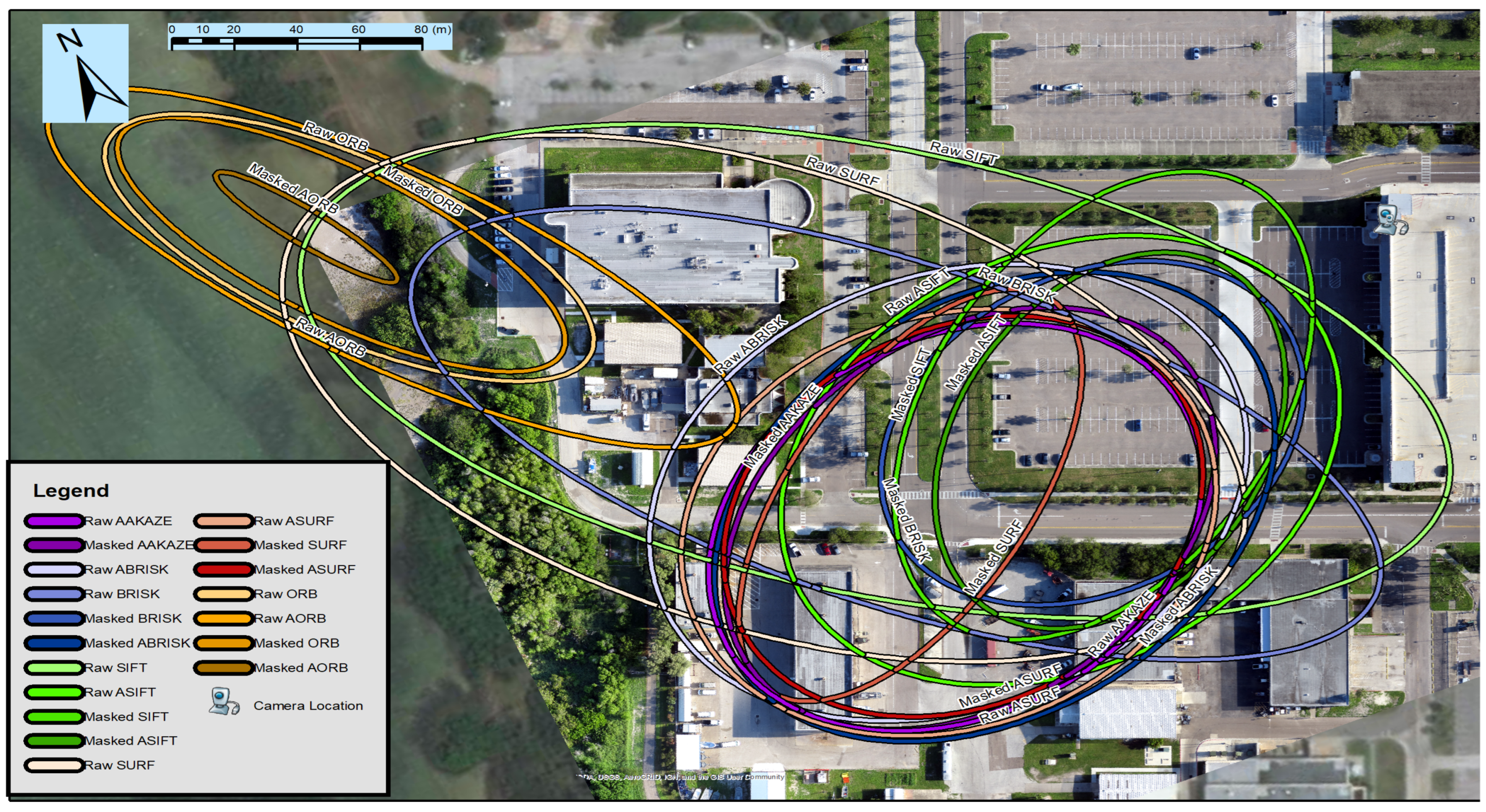
4.4. Automated Registration Results via Monoplotting

The results of this process are arranged by sequentially keypointing the low traffic video sample frames and matching them to the UAS orthomosaic then applying the same iterative adjustment defined in Section 3.2 to compute an image registration, from which the video camera pose is derived. The methods tested are SIFT [26], SURF [25], ORB [21], AKAZE [70], BRISK [71] and an affine version of each (ASIFT, ASURF, AORB, ABRISK, AAKAZE) [35,36]. When referring to a keypointing method in this section, the reference refers to the collection of results recorded using the specific method (e.g., the SIFT method results refers to the perspective video frames and UAS orthomosaic which have been keypointed using the method, and the results of the keypoint matching for each frame to the orthomosaic).
There are two sets of passes performed with each method, as described in Section 3.4, one where the video frame was keypointed in it’s entirety, referred to as raw, and the other where the keypointing process used the region of interest defined in Section 3.3 as a mask to isolate keypoints to the relevant ROI, referred to as masked. Figure 12 shows the masked video frames with affine keypointing methods applied to them would suggest clear improvements to acquiring matches and effective inliers between video frames and the orthomosaic for computing image registrations.
However, when computing the camera pose solution from keypoint matches per frame, the distribution of poses computed across all 6646 frames of Sample 1 varies far more widely than expected from the ground truth position and the position estimated in Section 4.1. The estimated position of the camera from using manually annotated point pairs in the single image monoplotting process is visualized in Figure 13, measured at 1.14 m distance away from the ground truth position using a total station. Figure 13 visualizes the distribution of the camera position estimation results across all methods, categorized by dataset, with multiple inset sections to highlight the extreme range which camera pose estimations covered, as well as the sparse number of results that even come close to the correct result. Figure 14 quantifies the standard deviation of camera position estimation in two dimensions, categorized by the dataset type and the keypointing method applied, which shows several interesting trends and patterns present in each method. A single position estimation, out of 119,628 total estimations across all permutations of methods and constraints, was within one meter of the ground truth position. Two additional estimations were within two meters of the ground truth position, and a dozen total estimations fall within the five meter range. All most nearby position estimations were oriented correctly, while position estimations farther away were oriented opposite.
Interestingly, ORB-based keypoint detection and matching methods were the most consistently selective about what they would identify as keypoints, but also detected the fewest keypoints of any method, which greatly reduced the number of matches made and thus the number of inliers computed to extremely low values as shown in Figure 12. Results suggest that its performance would be below average in this application. This is confirmed in Figure 14, which shows that the deviation of ORB pose estimations focuses around the northern corner of the study area, clearly in error. Henceforth, any generalized statements can be considered to be ignoring any ORB-based results.
Figure 14 also shows that the standard versions of the SIFT, SURF, and BRISK methods applied to the raw dataset were the least consistent at approaching a single solution, even an incorrect one. The affine versions of the same methods on the raw dataset were considerably more consistent, generally covering approximately half as much area in terms of deviation. Both standard and affine methods applied to the masked dataset were at least equivalent if not a slight improvement in consistency over the raw affine processing. Slight variances in total numbers of frames are due to failures to find enough inlier matches to compute a pose.
It is of note that this is an extremely challenging scene to register correctly with unmodified keypointing algorithms alone, as there are multiple kinds of repeated features and otherwise largely featureless areas, with an extreme pose transition between the two views. Because of these factors, results of attempts to automate monoplotting without modification of keypoint matching logic, are considerably less than ideal. Of the 119,628 pose estimations performed across all methods and constraints, 12,160 ( 10.2 % ) of the pose estimations did not fall within the bounds of the data collection area, let alone the study area, which only contained 36,646 ( 30.6 % ) pose estimations, leaving 70,822 ( 59.2 % ) pose estimations within the data collection area but outside the study area. Furthermore, the vast majority of the estimations within the data collection area focus upon solutions which trend towards either the north-western corner of the data collection area, or the south-western corner of the study area, as shown by the ellipses of standard deviation computed in Figure 14.
In the ideal case, there would be discussion of how far to either side of the camera origin computed position solutions ended up deviating as a statistical distribution. However, as the majority of computed position solutions ended up nowhere close to the perspective camera ground truth position on the UAS orthomosaic, it is more effective to visualize this phenomenon as a histogram. Distances from the camera origin are calculated by 3D vector subtraction relative to the ground truth position, categorized by method, shown in Figure 15 as a percentage of frames within a given distance from the ground truth position. In the ideal case, Figure 15 would have a strong leftward skew for all methods, falling off quickly as distance from the perspective camera origin increases. Clearly, Figure 15 does not illustrate anything remotely close to the ideal case: SIFT, SURF, and their affine counterparts generally performed the best, with the strongest leftward skews indicating a closer general proximity to the ground truth position, but that in itself is an extremely generous statement given that less than 20% of the frames processed resolved to a pose within 100 m.
Rather than truly being inaccurate, the concentrations of computed positions shown in Figure 13 and Figure 14 potentially suggest that the 2D-3D solution for pose computation is preferring one of three degenerate solutions reflected over the center point of the perspective image projected into 3D space. Inspection into the computation process confirms that in nearly every case, a position close to the ground truth position was available, but for an indeterminate reason a degenerate result reflected across a plane similar in orientation to the camera plane but located at the ground position of the perspective view’s central pixel in 3D space was preferable, thus the results are presented as they were calculated. Our current theory is that this is an effect of attempting to reconcile the high transition tilt between the perspective and aerial views with some degree of keypoints matched in error, causing pose solutions to trend towards a minimum other than the desired target.

5. Discussion

The computer vision pipeline was successfully deployed, after some enhancement, and meeting certain conditions. Prior to implementing the automatic vertical occlusion detection so that more robust tracking logic could be implemented, the ability to track vehicles throughout the scene until they actually exited the camera view was almost zero percent in both video samples. Having an effective registration from monoplotting becomes paramount for accurately estimating the parameters of potentially occluded image areas effectively, as shown in Figure 6. Object detection results from the custom trained neural network were generally quite consistent compared to the hand-crafted annotation method, though it was common for automated methods to have multiple partial detections compared to a singular ground truth detection. However, this was largely due to the choice of tracking method which would affect the capacity for multiple object detections of vehicles navigating in regions of egress. There were several combinations of computer vision pipeline parameters that could run at or above input camera frame rate. A combination of detecting objects using Darknet and tracking on detected object centroids was a 1:1 match to ground truth in the low traffic sample. Multiple region constrained tracking algorithms also often achieved tracking stability within a deviation of 10% of the ground truth in the low traffic sample. However, high traffic scenes such as the second sample are likely to need more robust and generally fit models for vehicle detection, and tracking methods which are more resilient to spurious similar features.
The custom trained Darknet model developed for this application was only slightly faster than the full model, but rides the limit of being over-fit, likely due to limited training data and low spatial distribution of target classes in that limited training data. Additionally, a side effect of the tested tracking methods retaining their lock on vehicles in regions of egress could severely hamper detection of additional vehicles, due to close proximity of additional vehicle features and previously detected but dissimilar objects. Overall, the computer-vision pipeline could be rated as effective for the needs of relatively low traffic areas, or in regions with smaller scopes and moderate amounts of traffic. For larger scopes, such as the study area and a high amount of traffic, more robust methods are required to avoid issues with tracking stability in particular.
Figure 7 shows that an increasing number of points used for monoplotting does not necessarily provide registrations of increasing accuracy. Each successive combination of points used appears to narrow the focus of monoplotting solution in sub-meter increments, but also increases misalignment around the edges of the image. Camera calibration can temporarily correct these distortions until it changes enough to cause inaccuracy, however even the uncalibrated images appear to align well enough to provide workable coordinate transformations. Even a minimal five point registration appears to provide workable coordinate transformation accuracy against the given DSM, shown in red on Figure 7. The following discussion refers to the most accurate registration computed out of the test in Section 3.2, which is shown in the top purple layer of Figure 7. Monoplotting with a single image reference and manually selected points (without including the ground truth survey location as initial adjustment parameters) produced a relatively close pose estimation as shown in Figure 13; 1.14 m away from the ground truth location of the camera at a similar elevation. The accuracy of the single image registration was also remarkably good, demonstrating accurate and precise transformation from the perspective view onto the aerial orthomosaic throughout 70% of the visible parking lot regardless of vehicle orientation, and 99% of the visible lot could be accurately transformed if a vehicle was presented along its longest axis. Figure 2 shows that the vast majority of the travel area shown in perspective video, especially as distance from the camera origin increases, would have vehicles presented along their long axis, which could be transformed accurately across almost the entire parking lot. Typical travel paths for vehicles within the parking lot are at least oblique in their presentation, meaning that there are few regions where vehicles are actually presented on their short axis and in areas of the image with uncertainty greater than the axis dimensions. There is little overhead calculating coordinate transformations once the monoplotting solution is solved, making the coordinate transformations of vehicle locations captured in perspective video onto the UAS orthomosaic image as fast as the computer vision pipeline can run. Of note, an artifact of this arrangement of monoplotting and object detection means that the transformed coordinates of vehicles are derived from rays projected from the camera origin through the centroids of the detection boxes to the ground plane. Transformed positioning error introduced through this effect is independent of image registration error and thus can compound with it; however, in practice, it is only at the furthest locations in the image away from the camera origin that this starts to become a non-negligible effect.
Unfortunately, the automated monoplotting process appears to be particularly sensitive to mismatched keypoints, even using an iterative adjustment approach which can drop points to reduce errors. In an effort to reduce keypoint mismatches and improve pose accuracy, we tested five of the most popular keypointing methods, as well as their affine implementations using Yu et al. and Morel et al. general process [35,36]. Additionally, we tested the difference in results for all methods when sharing the constraint of a manually defined ground plane from Section 3.3 used as a keypoint matching mask, the effects of which are shown in Figure 12, Figure 13 and Figure 14. Of the 119,628 pose estimations produced from all methods tested, with and without the masking constraint, a single frame from the Masked ABRISK run computed what we would consider a good result for pose estimation, a sub-meter accuracy solution. However, that solution was an outlier for that particular combination of data and method type, and so not indicative of any particular suitability to the task. This extremely limited degree of success in acquiring even remotely accurate pose estimations from uninitialized positions was unexpected.
Although the single successful result indicates it is possible for the process to work, there is a compound chain of three effects theorized to be the primary source of error observed in pose estimation. First, while the number of mismatched keypoints was usually a small fraction of the total keypoints computed for an image, keypoint descriptors with unstable and/or incorrect matching behavior were rather uniformly interspersed with correct matches in each video frame. Because keypoints were computed for the aerial image once, without a specific focus or constraint on the parking lot area of interest by intentional design, common features could mismatch to features outside the study area. While we observed that roughly one keypoint per thousand would mismatch outside the study area bounds for the perspective imagery, leading to single digit counts of egregious mismatches for normal keypointing and double digit counts for affine keypointing, this did not occur commonly enough to cause concern in initial testing, especially as these were only a few mismatches to remain after RANSAC eliminated most of the more extreme outliers. However, these keypoint mismatches were often positioned well away from the edges of the working area. In this case study’s particular perspective to aerial viewpoint configuration, it is possible the iterative adjustment would first drop keypoints near the edges of the image for error correction, as shown in Figure 5, which would lend the most egregious mismatches more weight during adjustment.
Second, during the initial adjustment computation keypoints which could be dropped for error minimization were far more likely to be weak correct matches that contributed little to the final solution than actual mismatches due to sheer volume. Thus, any retained mismatches would contribute additional weight to the final solution with subsequent iterations unless they were promptly also dropped. Thirdly, inaccurate Z-values that would be retrieved from the DSM due to keypoint mismatching can also skew adjustment results. All these effects in combination can cause the iterative adjustment to pivot early into an incorrect local minimum with little chance of recovering a correct solution. While confidence in the DSM ground plane accuracy would suggest low if any error contribution to the monoplotting process from the DSM itself, that only applies if features are matched to areas that are part of the ground plane correctly.
In effect, even a moderate to low degree of mismatching within the study bounds due to the repetitive features can cause the initial pose estimation of the iterative adjustment performed by the automated monoplotting process to be closer to a degenerate solution than a correct one, particularly if there are mismatches retained to features outside of the study area. Successive iterations would further degrade the proximity of the final result to its expected location as the adjustment drops points which would strengthen the actual solution in pursuit of a degenerate one, until all that remains is a mess of coordinates that have no real resolution or that actually resolve on a degenerate solution. This is somewhat visible in Figure 13 as the masked frame keypoints trend towards a degenerate solution, localized around the center of an “X” shape, while the unmasked keypoints mostly cluster around the area in a cloud without a definite shape.

6. Conclusions

Of the three contributions outlined in Section 1, it was possible to demonstrate a computer vision pipeline which would function in an accurate way for detecting vehicles as they entered or exited the study area. Without the enhancement of the occlusion detection and handling made possible by integration of the products necessary for monoplotting from the second contribution, it could still function as a serviceable application for monitoring/counting vehicle egress in the parking lot. However, tracking vehicles while they traverse the broader scope of an area would only be feasible with an unobstructed view of that area. In terms of vehicle detection abilities, the custom trained network performed as well as the fully trained model with a minimal improvement to processing time, and detected the vast majority of vehicles passing through ingress and egress zones. Notably, any object detection network with the appropriate categories could be swapped out for the Darknet models applied in this study. In terms of vehicle tracking, the KCF and TLD methods were the most effective at discrete vehicle tracking. Although the centroid tracking method was generally faster than either, it struggled with keeping vehicles discretely tracked and jumped from one vehicle to another frequently. Ultimately, combining the data annotation method with the object detection and tracking methods could yield extremely effective motion-based tracking results, with a validation layer provided by Darknet and a tracking method of choice for a minimal performance impact in combination with a static camera configuration.
The second contribution was able to extend the computer vision pipeline by making it possible to track vehicles which could become partially occluded by vertical structures. The tested object tracking algorithms were quite effective under simple conditions, but the practical constraints of occlusions demonstrated how delicate some trackers were to occluded subjects, requiring the implementation of occlusion detection. Occlusion regions around mostly-vertical features could be automatically extracted and converted into polygonal regions in the perspective view using the monoplotted relationship between the perspective and UAS orthomosaic images, instead of a relatively expensive viewshed computation on the DSM. This was deemed more effective as there was the expectation that the position of the occluding regions would have to be updated frequently if the perspective video origin was manipulated.
The third contribution explored the results of a best case scenario: just how accurate coordinate transformation monoplotting could be without being able to calibrate the perspective camera geometry. This was determined using a single video frame and a semi-automatic process to assist manual identification and pairing of keypoints between the perspective video and UAS orthomosaic. By separating the manually identified points into multiple recursively growing sets, it was possible to determine that while some transformation variation occurred, overall the results did not vary much between the smallest and largest collections of points used to compute the image registration. In theory, so long as the minimum number of points required were matched correctly, the iteration adjustment of the monoplotting process would lock in on a reasonably good solution. The best case image registration demonstrated that it was possible to accurately transform vehicles visible on their long axis through 99.6% of the study area, and through 70.5% of the study area along their short axis. Only a very small percentage of the visible study area would actually be unusable in terms of coordinate transformations, and it was concentrated in very small sections, in which entire vehicles would just barely fit. Overall, coordinate transformation accuracy would be more than accurate enough for tracking vehicle travel with a reasonably high degree of confidence.
The experiment which explored full automation of the monoplotting process from an uninitialized starting location demonstrated that while it is theoretically possible to accomplish (a single high accuracy pose estimation was computed out of 119,628 tested frames), the stability of the solution can vary widely based on the keypointing method used and the opportunity to apply feature masks. This ultimately is a failure, though one that provides insights into the causes of solution instability and a foundation for continuation of future work. Results showed that if a minimum number of correct matches were made, the iterative adjustment would be able to home in on a pose solution; however, the degree to which mismatching could occur in the full video samples and the impact of the effects of mismatched keypoints on the fidelity of the solution was underestimated. Specifically, there was a combination of effects that had strong negative impacts on the automated monoplotting adjustment. When mismatched points have stronger responses than correctly matched keypoints, the spatial range of some mismatched points extends far beyond the typical range of the target domain, and mismatched keypoints are retained early in the iterative adjustment. This can cause multiple mismatched points to match to a single point, which forces all keypoint matches to be dropped from consideration, including possibly correct keypoint matches; or correct keypoint matches may be dropped during adjustment in favor of mismatches. The iterative adjustment performed by the monoplotting process should be able to drop some incorrectly matched points as low accuracy, but if enough mismatches are consistent, then the iterative adjustment will trend towards a degenerate solution, away from what would be the closest correct pose estimation. Compounded with a challenging scene containing frequently repeated image features, partially deformable subjects (palm tree fronds that change with the wind), and the presence of a high degree of transition tilt between the perspective view and aerial orthomosaic, the extremely limited degree of success in acquiring even remotely accurate pose estimations, and by extent usable image registrations, suggests that descriptor matching methods alone lack the necessary context to consistently leverage the available information to determine accurate relative pose without masking both aerial and perspective image views.
Future work on this application could touch on several areas of study. If a reliable solution for automating monoplotting can be achieved, then the framework should be able to support integration of multiple cameras over a much larger area, such as the full campus survey. There have been a number of advances in neural network object tracking tasks which could potentially be drop-in replacements for the algorithmic object trackers used in this paper that are more resilient to object occlusion, as well as improvements to object detection networks. This could potentially allow elimination of the automated occlusion process within the VirtuaLot framework.
Current focus is directed towards developing a fast keypoint matching method which retains a degree of spatial context awareness through methods similar to the work of Zhao et al. [74], though this presents its own challenges. Such context awareness could also be achieved by applying a convolutional neural network across the entirety of perspective video frames to identify areas which have a high probability of containing deformable image features, and excluding those features from the keypoint matching process, in combination with logical checks to ensure that keypoints are matched in a logically consistent orientation between image spaces. In conjunction with increased keypoint density from fully affine keypoint processing, better results from matching methods could potentially enable the composition of multiple partial image registrations to improve coordinate transformation accuracy, somewhat similar to Produit [41]. Alternatively, the application of linear features similar to Boerner [4] could be integrated with, or replace, keypoints through collinear feature recognition to provide better parameters for computing the pose of a terrestrial video camera using nadir perspective aerial imagery. Ultimately, the VirtuaLot framework could potentially serve as a foundation which could provide the data necessary to power frameworks similar to [75].

Author Contributions

Conceptualization, B.K.; methodology, B.K.; software, B.K.; validation, B.K.; formal analysis, B.K. and M.S.; investigation, B.K.; resources, B.K.; data curation, B.K.; writing—original draft preparation, B.K. and M.S.; writing—review and editing, B.K., M.S. and S.A.K.; visualization, B.K. and S.A.K.; supervision, M.S.; project administration, M.S.; funding acquisition, N/A. All authors have read and agreed to the published version of the manuscript.

Funding

This research received no external funding.

Data Availability Statement

Data may be available on request due to privacy restrictions.

Acknowledgments

Thanks are extended to: Texas A&M Corpus Christi University Police Department: for generous access to their camera system; The TAMUCC Measurement Analytics Lab (MANTIS): for generously providing up-to-date aerial imagery products; Maryam Rahnemoonfar (Formerly of the TAMUCC BINA Lab) for initial review and feedback on the computer vision pipeline.

Conflicts of Interest

The authors declare no conflict of interest.

References

  1. Chu, T.; Guo, N.; Backén, S.; Akos, D. Monocular Camera/IMU/GNSS Integration for Ground Vehicle Navigation in Challenging GNSS Environments. Sensors 2012, 12, 3162–3185. [Google Scholar] [CrossRef] [PubMed]
  2. Gupton, N. The Science of Self-Driving Cars; Technical Report; The Franklin Institute: Philadelphia, PA, USA, 2019. [Google Scholar]
  3. Behzadan, A.H.; Kamat, V.R. Georeferenced Registration of Construction Graphics in Mobile Outdoor Augmented Reality. J. Comput. Civ. Eng. 2007, 21, 247–258. [Google Scholar] [CrossRef]
  4. Boerner, R.; Kröhnert, M. Brute Force Matching Between Camera Shots and Synthetic Images From Point Clouds. ISPRS Int. Arch. Photogramm. Remote Sens. Spat. Inf. Sci. 2016, XLI-B5, 771–777. [Google Scholar] [CrossRef] [Green Version]
  5. Oh, T.; Lee, D.; Kim, H.; Myung, H. Graph Structure-Based Simultaneous Localization and Mapping Using a Hybrid Method of 2D Laser Scan and Monocular Camera Image in Environments with Laser Scan Ambiguity. Sensors 2015, 15, 15830–15852. [Google Scholar] [CrossRef] [Green Version]
  6. Mair, E.; Strobl, K.H.; Suppa, M.; Burschka, D. Efficient camera-based pose estimation for real-time applications. In Proceedings of the 2009 IEEE/RSJ International Conference on Intelligent Robots and Systems, St. Louis, MO, USA, 10–15 October 2009. [Google Scholar] [CrossRef] [Green Version]
  7. Szelag, K.; Kurowski, P.; Bolewicki, P.; Sitnik, R. Real-time camera pose estimation based on volleyball court view. Opto-Electron. Rev. 2019, 27, 202–212. [Google Scholar] [CrossRef]
  8. Mur-Artal, R.; Montiel, J.M.M.; Tardos, J.D. ORB–SLAM: A Versatile and Accurate Monocular SLAM System. IEEE Trans. Robot. 2015, 31, 1147–1163. [Google Scholar] [CrossRef] [Green Version]
  9. Cavallari, T.; Golodetz, S.; Lord, N.; Valentin, J.; Prisacariu, V.; Stefano, L.D.; Torr, P.H. Real-Time RGB-D Camera Pose Estimation in Novel Scenes using a Relocalisation Cascade. IEEE Trans. Pattern Anal. Mach. Intell. 2019, 42, 2465–2477. [Google Scholar] [CrossRef] [Green Version]
  10. Mishkin, D.; Matas, J.; Perdoch, M. MODS: Fast and Robust Method for Two-View Matching. Comput. Vis. Image Underst. 2016, 141, 81–93. [Google Scholar] [CrossRef] [Green Version]
  11. Bartol, K.; Bojanić, D.; Pribanić, T.; Petković, T.; Donoso, Y.D.; Mas, J.S. On the Comparison of Classic and Deep Keypoint Detector and Descriptor Methods. In Proceedings of the 2019 11th International Symposium on Image and Signal Processing and Analysis (ISPA), Dubrovnik, Croatia, 23–25 September 2020; pp. 64–69. [Google Scholar] [CrossRef]
  12. Wu, C. Towards Linear-Time Incremental Structure from Motion. In Proceedings of the 2013 International Conference on 3D Vision, Seattle, WA, USA, 29 June–1 July 2013. [Google Scholar] [CrossRef] [Green Version]
  13. Slocum, R.K.; Parrish, C.E. Simulated Imagery Rendering Workflow for UAS-Based Photogrammetric 3D Reconstruction Accuracy Assessments. Remote Sens. 2017, 9, 396. [Google Scholar] [CrossRef] [Green Version]
  14. Mouragnon, E.; Lhuillier, M.; Dhome, M.; Dekeyser, F.; Sayd, P. Generic and real-time structure from motion using local bundle adjustment. Image Vis. Comput. 2009, 27, 1178–1193. [Google Scholar] [CrossRef] [Green Version]
  15. Strasdat, H.; Montiel, J.M.M.; Davison, A.J. Real-time monocular SLAM: Why filter? In Proceedings of the 2010 IEEE International Conference on Robotics and Automation, Anchorage, AK, USA, 3–7 May 2010. [Google Scholar] [CrossRef] [Green Version]
  16. Lee, A.H.; Lee, S.H.; Lee, J.Y.; Choi, J.S. Real-time camera pose estimation based on planar object tracking for augmented reality environment. In Proceedings of the 2012 IEEE International Conference on Consumer Electronics (ICCE), Las Vegas, NV, USA, 13–16 January 2012. [Google Scholar] [CrossRef]
  17. Liu, Y.; Chen, X.; Gu, T.; Zhang, Y.; Xing, G. Real-time camera pose estimation via line tracking. Vis. Comput. 2018, 34, 899–909. [Google Scholar] [CrossRef]
  18. Chakravarty, P.; Narayanan, P.; Roussel, T. GEN-SLAM: Generative Modeling for Monocular Simultaneous Localization and Mapping. arXiv 2019, arXiv:1902.02086v1. [Google Scholar]
  19. Schmuck, P.; Chli, M. CCM-SLAM: Robust and efficient centralized collaborative monocular simultaneous localization and mapping for robotic teams. J. Field Robot. 2018, 36, 763–781. [Google Scholar] [CrossRef] [Green Version]
  20. Wu, J.; Cui, Z.; Sheng, V.S.; Zhao, P.; Su, D.; Gong, S. A Comparative Study of SIFT and its Variants. Meas. Sci. Rev. 2013, 13, 122–131. [Google Scholar] [CrossRef] [Green Version]
  21. Rublee, E.; Rabaud, V.; Konolige, K.; Bradski, G. ORB: An efficient alternative to SIFT or SURF. In Proceedings of the 2011 International Conference on Computer Vision, Barcelona, Spain, 6–13 November 2011. [Google Scholar] [CrossRef]
  22. Tola, E.; Lepetit, V.; Fua, P. DAISY: An Efficient Dense Descriptor Applied to Wide-Baseline Stereo. IEEE Trans. Pattern Anal. Mach. Intell. 2010, 32, 815–830. [Google Scholar] [CrossRef]
  23. Tola, E.; Lepetit, V.; Fua, P. A fast local descriptor for dense matching. In Proceedings of the 2008 IEEE Conference on Computer Vision and Pattern Recognition, Anchorage, AK, USA, 23–28 June 2008. [Google Scholar] [CrossRef] [Green Version]
  24. Aanæs, H.; Dahl, A.L.; Pedersen, K.S. Interesting Interest Points. Int. J. Comput. Vis. 2011, 97, 18–35. [Google Scholar] [CrossRef]
  25. Bay, H.; Tuytelaars, T.; Van Gool, L. SURF: Speeded Up Robust Features. In Proceedings of the Computer Vision—ECCV 2006, Graz, Austria, 7–13 May 2006; Leonardis, A., Bischof, H., Pinz, A., Eds.; Springer: Berlin/Heidelberg, Germany, 2006; pp. 404–417. [Google Scholar]
  26. Lowe, D.G. Distinctive Image Features from Scale-Invariant Keypoints. Int. J. Comput. Vis. 2004, 60, 91–110. [Google Scholar] [CrossRef]
  27. Shi, J.; Tomasi, C. Good Features To Track. Comput. Vis. Pattern Recognit. 1994, 593–600. [Google Scholar] [CrossRef]
  28. Guo, Y.; Bennamoun, M.; Sohel, F.; Lu, M.; Wan, J.; Kwok, N.M. A Comprehensive Performance Evaluation of 3D Local Feature Descriptors. Int. J. Comput. Vis. 2015, 116, 66–89. [Google Scholar] [CrossRef]
  29. Hartley, R.; Zisserman, A. Multiple View Geometry in Computer Vision, 2nd ed.; Cambridge University Press: Cambridge, MA, USA, 2003. [Google Scholar]
  30. Moulon, P.; Monasse, P.; Marlet, R. Adaptive Structure from Motion with a Contrario Model Estimation. In Proceedings of the Computer Vision—ACCV 2012, Daejeon, Korea, 5–9 November 2012; Lee, K.M., Matsushita, Y., Rehg, J.M., Hu, Z., Eds.; Springer: Berlin/Heidelberg, Germany, 2013; pp. 257–270. [Google Scholar]
  31. Kendall, A.; Grimes, M.; Cipolla, R. PoseNet: A Convolutional Network for Real-Time 6-DOF Camera Relocalization. arXiv 2015, arXiv:1505.07427. [Google Scholar]
  32. Bae, H.; Golparvar-Fard, M.; White, J. High-precision vision-based mobile augmented reality system for context-aware architectural, engineering, construction and facility management (AEC/FM) applications. Vis. Eng. 2013, 1. [Google Scholar] [CrossRef] [Green Version]
  33. Cai, G.R.; Jodoin, P.M.; Li, S.Z.; Wu, Y.D.; Su, S.Z.; Huang, Z.K. Perspective-SIFT: An efficient tool for low-altitude remote sensing image registration. Signal Process. 2013, 93, 3088–3110. [Google Scholar] [CrossRef]
  34. Wilson, K.; Snavely, N. Robust Global Translations with 1DSfM. In Proceedings of the European Conference on Computer Vision (ECCV), Zurich, Switzerland, 6–12 September 2014. [Google Scholar]
  35. Morel, J.M.; Yu, G. ASIFT: A New Framework for Fully Affine Invariant Image Comparison. SIAM J. Imaging Sci. 2009, 2, 438–469. [Google Scholar] [CrossRef] [Green Version]
  36. Yu, G.; Morel, J.M. ASIFT: An Algorithm for Fully Affine Invariant Comparison. Image Process. Line 2011, 1, 11–38. [Google Scholar] [CrossRef] [Green Version]
  37. Maier, R.; Schaller, R.; Cremers, D. Efficient Online Surface Correction for Real-time Large-Scale 3D Reconstruction. arXiv 2017, arXiv:1709.03763v1. [Google Scholar]
  38. Yi, K.M.; Trulls, E.; Lepetit, V.; Fua, P. LIFT: Learned Invariant Feature Transform. In Proceedings of the European Conference On Computer Vision, Amsterdam, The Netherlands, 11–14 October 2016. [Google Scholar]
  39. Strausz, D.A., Jr. An Application of Photogrammetric Techniques to the Measurement of Historic Photographs; Oregon State University: Corvallis, OR, USA, 2001. [Google Scholar]
  40. Bozzini, C.; Conedera, M.; Krebs, P. A New Monoplotting Tool to Extract Georeferenced Vector Data and Orthorectified Raster Data from Oblique Non-Metric Photographs by C. Bozzini, M. Conedera, P. Krebs. Int. J. Herit. Digit. Era 2012, 1, 499–518. [Google Scholar] [CrossRef]
  41. Produit, T.; Tuia, D. An open tool to register landscape oblique images and and generate their synthetic model. In Proceedings of the Open Source Geospatial Research and Education Symposium (OGRS), Yverdon les Bains, Switzerland, 24–26 October 2012; pp. 170–176. [Google Scholar]
  42. Petrasova, A.; Hipp, J.A.; Mitasova, H. Visualization of Pedestrian Density Dynamics Using Data Extracted from Public Webcams. ISPRS Int. J. Geo-Inf. 2019, 8, 559. [Google Scholar] [CrossRef] [Green Version]
  43. Chen, X.; Wang, Z.; Hua, Q.; Shang, W.L.; Luo, Q.; Yu, K. AI-Empowered Speed Extraction via Port-Like Videos for Vehicular Trajectory Analysis. IEEE Trans. Intell. Transp. Syst. 2022, 1–12. [Google Scholar] [CrossRef]
  44. Koskowich, B.J.; Rahnemoonfai, M.; Starek, M. Virtualot—A Framework Enabling Real-Time Coordinate Transformation & Occlusion Sensitive Tracking Using UAS Products, Deep Learning Object Detection & Traditional Object Tracking Techniques. In Proceedings of the IGARSS—2018 IEEE International Geoscience and Remote Sensing Symposium, Valencia, Spain, 22–27 July 2018. [Google Scholar] [CrossRef]
  45. Jiang, Q.; Liu, Y.; Yan, Y.; Xu, P.; Pei, L.; Jiang, X. Active Pose Relocalization for Intelligent Substation Inspection Robot. IEEE Trans. Ind. Electron. 2022, 99, 1–10. [Google Scholar] [CrossRef]
  46. Zhang, X.; Shi, X.; Luo, X.; Sun, Y.; Zhou, Y. Real-Time Web Map Construction Based on Multiple Cameras and GIS. ISPRS Int. J. Geo-Inf. 2021, 10, 803. [Google Scholar] [CrossRef]
  47. Han, S.; Dong, X.; Hao, X.; Miao, S. Extracting Objects’ Spatial–Temporal Information Based on Surveillance Videos and the Digital Surface Model. ISPRS Int. J. Geo-Inf. 2022, 11, 103. [Google Scholar] [CrossRef]
  48. Luo, X.; Wang, Y.; Cai, B.; Li, Z. Moving Object Detection in Traffic Surveillance Video: New MOD-AT Method Based on Adaptive Threshold. ISPRS Int. J. Geo-Inf. 2021, 10, 742. [Google Scholar] [CrossRef]
  49. Cao, X.; Wu, C.; Yan, P.; Li, X. Linear SVM classification using boosting HOG features for vehicle detection in low-altitude airborne videos. In Proceedings of the 2011 18th IEEE International Conference on Image Processing, Brussels, Belgium, 11–14 September 2011. [Google Scholar] [CrossRef]
  50. Choi, J.; Chang, H.J.; Yoo, Y.J.; Choi, J.Y. Robust moving object detection against fast illumination change. Comput. Vis. Image Underst. 2012, 116, 179–193. [Google Scholar] [CrossRef]
  51. Dollar, P.; Wojek, C.; Schiele, B.; Perona, P. Pedestrian Detection: An Evaluation of the State of the Art. IEEE Trans. Pattern Anal. Mach. Intell. 2012, 34, 743–761. [Google Scholar] [CrossRef]
  52. Redmon, J.; Farhadi, A. YOLOv3: An Incremental Improvement. arXiv 2018, arXiv:1804.02767v1. [Google Scholar]
  53. Simon, M.; Milz, S.; Amende, K.; Gross, H.M. Complex-YOLO: Real-time 3D Object Detection on Point Clouds. arXiv 2018, arXiv:1803.06199v2. [Google Scholar]
  54. Zhao, Z.Q.; Zheng, P.; Xu, S.T.; Wu, X. Object Detection with Deep Learning: A Review. arXiv 2018, arXiv:cs.CV/1807.05511. [Google Scholar] [CrossRef] [PubMed] [Green Version]
  55. Kalal, Z.; Mikolajczyk, K.; Matas, J. Tracking-Learning-Detection. IEEE Trans. Pattern Anal. Mach. Intell. 2010, 34, 1409–1422. [Google Scholar] [CrossRef] [Green Version]
  56. Kalal, Z.; Mikolajczyk, K.; Matas, J. Forward-backward error: Automatic detection of tracking failures. In Proceedings of the 2010 20th International Conference on Pattern Recognition, Istanbul, Turkey, 23–26 August 2010; pp. 2756–2759. [Google Scholar]
  57. Babenko, B.; Yang, M.H.; Belongie, S. Visual Tracking with Online Multiple Instance Learning. In Proceedings of the 2009 IEEE Conference on Computer Vision and Pattern Recognition, Miami, FL, USA, 20–25 June 2009. [Google Scholar] [CrossRef]
  58. Tao, M.; Bai, J.; Kohli, P.; Paris, S. SimpleFlow: A Non-iterative, Sublinear Optical Flow Algorithm. Comput. Graph. Forum 2012, 31, 345–353. [Google Scholar] [CrossRef]
  59. Henriques, J.F.; Caseiro, R.; Martins, P.; Batista, J. High-Speed Tracking with Kernelized Correlation Filters. IEEE Trans. Pattern Anal. Mach. Intell. 2015, 37, 583–596. [Google Scholar] [CrossRef] [PubMed] [Green Version]
  60. Xiang, Y.; Alahi, A.; Savarese, S. Learning to Track: Online Multi-object Tracking by Decision Making. In Proceedings of the 2015 IEEE International Conference on Computer Vision (ICCV), Santiago, Chile, 7–13 December 2015. [Google Scholar] [CrossRef] [Green Version]
  61. Kristan, M.; Matas, J.; Leonardis, A.; Vojir, T.; Pflugfelder, R.; Fernandez, G.; Nebehay, G.; Porikli, F.; Čehovin, L. A Novel Performance Evaluation Methodology for Single-Target Trackers. IEEE Trans. Pattern Anal. Mach. Intell. 2016, 38, 2137–2155. [Google Scholar] [CrossRef] [PubMed] [Green Version]
  62. Bertinetto, L.; Valmadre, J.; Henriques, J.F.; Vedaldi, A.; Torr, P.H.S. Fully-Convolutional Siamese Networks for Object Tracking. In Computer Vision—ECCV 2016 Workshops. ECCV 2016; Hua, G., Jégou, H., Eds.; Lecture Notes in Computer Science; Springer: Cham, Switzerland, 2016; Volume 9914, pp. 850–865. [Google Scholar] [CrossRef] [Green Version]
  63. Valmadre, J.; Bertinetto, L.; Henriques, J.; Vedaldi, A.; Torr, P.H.S. End-To-End Representation Learning for Correlation Filter Based Tracking. In Proceedings of the The IEEE Conference on Computer Vision and Pattern Recognition (CVPR), Honolulu, HI, USA, 21–26 July 2017. [Google Scholar]
  64. Ondatec. Polycarbonate Systems. Available online: https://www.stabiliteuropa.com/sites/default/files/ondatec_english.pdf (accessed on 2 August 2022).
  65. Amerilux. Glossary. Available online: https://ameriluxinternational.com/wp-content/uploads/2021/pdf-downloads/general-resources/amerilux-glossary.pdf (accessed on 2 August 2022).
  66. Redmon, J.; Farhadi, A. YOLO9000: Better, Faster, Stronger. In Proceedings of the The IEEE Conference on Computer Vision and Pattern Recognition (CVPR), Honolulu, HI, USA, 21–26 July 2017; University of Washington, Allen Institute for AI: Washington, DC, USA, 2016. [Google Scholar]
  67. Grabner, H.; Grabner, M.; Bischof, H. Real-Time Tracking via On-line Boosting. In Proceedings of the British Machine Vision Conference 2006, Edinburgh, UK, 4–7 September 2006; 2006. [Google Scholar] [CrossRef] [Green Version]
  68. Everingham, M.; Van Gool, L.; Williams, C.K.I.; Winn, J.; Zisserman, A. The PASCAL Visual Object Classes Challenge 2012 (VOC2012) Results. 2012. Available online: http://www.pascal-network.org/challenges/VOC/voc2012/workshop/index.html (accessed on 2 August 2022).
  69. Duda, R.O.; Hart, P.E. Use of the Hough transformation to detect lines and curves in pictures. Commun. ACM 1972, 15, 11–15. [Google Scholar] [CrossRef]
  70. Alcantarilla, P.F.; Bartoli, A.; Davison, A.J. KAZE Features. In Proceedings of the Computer Vision—ECCV 2012, Florence, Italy, 7–13 October 2012; Springer: Berlin/Heidelberg, Germany, 2012; pp. 214–227. [Google Scholar] [CrossRef]
  71. Leutenegger, S.; Chli, M.; Siegwart, R.Y. BRISK: Binary Robust invariant scalable keypoints. In Proceedings of the 2011 International Conference on Computer Vision, Barcelona, Spain, 6–13 November 2011; Volume 22, pp. 2548–2555. [Google Scholar] [CrossRef] [Green Version]
  72. Texas Department of Licensing and Regulation. Texas Accessibility Standards, Chapter 5. In Texas Government Code Chapter 469; Texas Department of Licensing and Regulation: Austin, TX, USA, 2012; p. 110. [Google Scholar]
  73. Grand Prairie, Texas Planning Department. Appendix D: Parking Layout and Design standards. In Unified Development Code; Grand Prairie, Texas Planning Department: Grand Prairie, TX, USA, 2003; pp. 4–16. [Google Scholar]
  74. Zhao, X.; He, Z.; Zhang, S. Improved keypoint descriptors based on Delaunay triangulation for image matching. Opt. Int. J. Light Electron Opt. 2014, 125. [Google Scholar] [CrossRef]
  75. Liu, X.; Qu, X.; Ma, X. Improving flex-route transit services with modular autonomous vehicles. Transp. Res. Part Logist. Transp. Rev. 2021, 149, 102331. [Google Scholar] [CrossRef]
Figure 1. An example aerial UAS orthomosaic that provides the X, Y coordinates for monoplotting features which are combined with the Z values from the DSM to compute the registration between the perspective and aerial views. The parking lot of interest is outlined in orange, with an aerial map of the TAMUCC campus inset.
Remotesensing 14 05451 g001
Figure 2. View of the study area from the perspective camera. Regions of the image where vehicle ingress/egress are expected are outlined in blue—there is no significance to the box thickness around each region, it is an artifact of the GUI tool developed to accelerate region definition.
Remotesensing 14 05451 g002
Figure 3. A high-level breakdown of the methodology and how the processes interact with one another in terms of data flow.
Remotesensing 14 05451 g003
Figure 4. Visualization of the monoplotting principle, and how the arrangement of camera origin, image plane, and world space are determined through the collinearity Equations [40].
Remotesensing 14 05451 g004
Figure 5. 399 manually annotated point pairs, with coordinates shown on the aerial image. Registration was tested for variance over successively larger sets of points, determined by group number. Points which were regularly dropped during the computation process to reduce transformation error are visualized as blue crosses.
Remotesensing 14 05451 g005
Figure 8. The amount of error present for each control point computed by the solution using all available control points. Errors less than 1.33 m are visualized but not labelled.
Remotesensing 14 05451 g008
Figure 9. Transformation accuracy from each perspective pixel to coordinates on the aerial image, interpolated by inverse distance weighting.
Remotesensing 14 05451 g009
Figure 10. Transformation accuracy qualified for vehicles detected by the computer vision pipeline. Coordinates in the blue region are estimated to be accurate within the limits of the width of a small vehicle, while coordinates in the green region will be accurate to within the length of a short vehicle. Coordinates in yellow regions are likely to be outside those dimensions.
Remotesensing 14 05451 g010
Figure 11. A visualization of the transformed coordinate accuracy output from the computer vision pipeline combined with the results of the monoplotting registration. The low traffic patterns are shown in red, and the high traffic patterns in blue. Note that as distance from the camera origin in the top right increases, coordinate transformations become less stable. There are also some triangular shapes present in the blue tracking lines which can be cross-referenced with Figure 8 and Figure 9 to identify the effects of lens imperfections.
Remotesensing 14 05451 g011
Figure 12. The average, standard deviation, and outliers of the number of keypoint matches and inliers computed across the entire sample, arranged by method and dataset.
Remotesensing 14 05451 g012
Figure 13. Categorization of pose estimation positions linked to raster pixels, shown as positions computed for the raw and masked version of the sample for all methods. The main map focuses on the data collection area, the orange inset focuses on the study area, and the purple inset focuses specifically on the area where the camera is present.
Remotesensing 14 05451 g013
Figure 14. The standard deviations of position estimations in 2D, categorized by dataset and keypoint method.
Remotesensing 14 05451 g014
Figure 15. A histogram of distances to ground truth pose computed across the sample. Note that an intentional axis break exists between 40 and 80% to clarify the distribution of lower percentages while still visualizing the outliers.
Remotesensing 14 05451 g015
Table 1. Dataset Metadata.
SourceData
Set
Capture
Metadata
Positioning
Information
Recording
Date
Perspective Footage:
AXIS Q6044-E PTZ,
Weatherproof
housing;
1280 × 720 p @ 30 fps
Sample 1 Video:
Low Traffic;
(Reduced From
432 K Frames)
6646 Frames
≈3 m 30 s
≈1 vehicle/5 s
Sporadic
15 m above
ground plane,
≈20° below
horizon
observing
south west
December
2016
Sample 2 Video:
High Traffic
4616 Frames
≈2 m 30 s
≈1.5 vehicles/s
Constant Motion
Aerial Imagery:
SODA SenseFly
Camera on
eBee
UAS
Flight
Sensor Resolution: 20 MP
1565 Images; Avg. GSD: 2.78 cm
Image Resolution: 5472 × 3648 px;
nadir observing; 80% sidelap/70% endlap
Flying a back and
forth grid pattern
≈91 m altitude,
covering 1.32 km2
September
2017
Digital Surface Model
Derived from Aerial
Imagery Point Cloud
Post
Processed
Data
Resolution:
12,042 × 8684 px
@ 2.79 cm/px
91.44 m altitude
above ground,
observing nadir,
covering 0.029 km2
Georeferenced
Orthomosaic:
Region Of Interest
Table 2. This table displays the detection, tracking, and FPS performance of the ground truth and sample runs performed with different tracking methods. Each column cell describes the average performance and deviation of all parameter swept runs categorized by tracking method.
Sample 1Ground TruthObject Tracking Methods
BoostingCentroidKCFMedianFlowTLD
Detection Count46.1 +/− 12.9438.45 +/− 8.5749.67 +/− 8.6446.74 +/− 12.151.5 +/− 7.3938 +/− 7.07
Tracking Stability0.86 +/− 2.130.16 +/− 0.373.21 +/− 7.970.22 +/− 0.660.18 +/− 0.40.1 +/− 0.23
FPS18.63 +/− 9.5015.53 +/− 10.4329.06 +/− 16.0731.06 +/− 16.717.97 +/− 14.5825.28 +/− 15.79
Sample 1 Min-MaxGround TruthBoostingCentroidKCFMedianFlowTLD
Detection Rate (%)21.74–10026.09–54.3545.65–10021.74–67.3939.13–67.3923.91–50
Tracking Stability0.05–3.460.03–0.340.86–3.460.09–0.690.1–0.310.05–0.17
FPS3–44.55.8–48.416.7–1234–63.53–61.94.1–63.3
Sample 2Ground TruthBoostingCentroidKCFMedianFlowTLD
Detection Count4.15 +/− 4.086.84 +/− 6.297.67 +/− 15.143.56 +/− 1.123.62 +/− 0.752.86 +/− 0.79
Tracking Stability0.04 +/− 0.300.06 +/− 0.310.12 +/− 0.620.02 +/− 0.130.03 +/− 0.210.01 +/− 0.09
FPS23.3 +/− 10.2320.65 +/− 8.6625.63 +/− 15.6422.24 +/− 6.5122.33 +/− 6.8120.97 +/− 6.96
Sample 2 Min-MaxGround TruthBoostingCentroidKCFMedianFlowTLD
Detection Rate (%)0–1001.5–70–1002–62–52–5
Tracking Stability0–10.01–0.090–10–0.030.01–0.10–0.05
FPS4–42.54–27.94.6–104.44–30.14.1–29.74–29.8
Publisher’s Note: MDPI stays neutral with regard to jurisdictional claims in published maps and institutional affiliations.

