
Characterizing Forest Cover and Landscape Pattern Using Multi-Source Remote Sensing Data with Ensemble Learning

1
Ministry of Education Key Laboratory for Earth Surface Processes, College of Urban and Environmental Sciences, Peking University, Beijing 100871, China
2
Land Consolidation and Rehabilitation Center, Ministry of Natural Resources, Beijing 100035, China
*
Author to whom correspondence should be addressed.
Remote Sens. 2022, 14(21), 5470; https://0-doi-org.brum.beds.ac.uk/10.3390/rs14215470
Submission received: 23 July 2022
/
Revised: 9 September 2022
/
Accepted: 16 September 2022
/
Published: 30 October 2022
(This article belongs to the Special Issue Remote Sensing in Applied Ecology)
Abstract
:Accurate information on forest distribution is an essential basis for the protection of forest resources. Recent advances in remote sensing and machine learning have contributed to the monitoring of forest-cover distribution cost-effectively, but reliable methods for rapid forest-cover mapping over mountainous areas are still lacking. In addition, the forest landscape pattern has proven to be closely related to the functioning of forest ecosystems, yet few studies have explicitly measured the forest landscape pattern or revealed its driving forces in mountainous areas. To address these challenges, we developed a framework for forest-cover mapping with multi-source remote sensing data (Sentinel-1, Sentinel-2) and an automated ensemble learning method. We also designed a scheme for forest landscape pattern evaluation and driver attribution based on landscape metrics and random forest regression. Results in the Qilian Mountains showed that the proposed framework and scheme could accurately depict the distribution and pattern of forest cover. The overall accuracy of the obtained level-1 and level-2 forest-cover maps reached 95.49% and 78.05%, respectively. The multi-classifier comparison revealed that for forest classification, the ensemble learning method outperformed base classifiers such as LightGBM, random forests, CatBoost, XGBoost, and neural networks. Integrating multi-dimensional features, including spectral, phenological, topographic, and geographic information, helped distinguish forest cover. Compared with other land-cover products, our mapping results demonstrated high quality and rich spatial details. Furthermore, we found that forest patches in the Qilian Mountains were concentrated in the eastern regions with low-to-medium elevations and shady aspects. We also identified that climate was the critical environmental determent of the forest landscape pattern in the Qilian Mountains. Overall, the proposed framework and scheme have strong application potential for characterizing forest cover and landscape patterns. The mapping and evaluation results can further support forest resource management, ecological assessment, and regional sustainable development.
1. Introduction
Forests, as the largest biological resource bank on Earth, cover 31% of the global land surface and are essential for ecosystem service conservation and ecological protection [1]. Forests play a vital role in adjusting regional climate, conserving soil and water, increasing carbon storage, and maintaining biodiversity [2]. However, forests are increasingly threatened by factors such as climate change, fires, and fragmentation, and have undergone significant changes over the past few decades [3,4]. Timely and accurate information on forest cover is urgently needed to provide a direct means of monitoring forest changes and support for sustainable natural resource management, carbon-cycle research, and Earth-system modeling [5,6,7].
In recent years, remote sensing technology has become an important and effective tool for detecting forest extent, types, and changes. Compared with ground survey data, remote sensing data are easier to acquire and process and allows for a higher frequency. Based on remote sensing data, several forest-cover and -type products over large areas have been developed, such as the Global Forest Cover 2000 30-m-resolution map [1], European Forest Type 2015 20-m-resolution map [8], and Copernicus High Resolution Layers Forest 2018 10-m-resolution maps [9]. However, these products are often not up-to-date, due to the lack of input data and large realization time. At the same time, the full suitability of these products is often limited, as forest classification is particularly challenging in mountainous areas with complex topography.
Because of its fine spatial resolution, short revisit cycle, and rich bands, Sentinel satellite imagery is expected to contribute to rapid, large-scale forest information extraction [10]. Many studies have used Sentinel-2 time series to classify forest cover, forest type, tree species, etc., and achieved high accuracies. For example, Hemmerling et al. [11] found that the use of dense Sentinel-2 time series was critical for improved tree-species mapping in temperate forests. Hamrouni et al. [12] developed a Sentinel-2 poplar-detection index that provided an operational approach for monitoring the poplar resource over large areas. However, due to shadows and frequent cloud cover, the use of Sentinel-2 imagery is often limited in mountainous areas. In contrast, Sentinel-1 radar imagery is promising in this regard, considering its independence from weather conditions and daytime, for instance, with Sentinel-1’s temporal features of backscattering, Yu et al. [13] mapped forests over mountainous areas in northeast China, and Dostálová et al. [14] carried out Europe-wide forest classification. Recently, some other studies have analyzed the synergy of optical and radar data in forest classification through the combined use of Sentinel-1 and Sentinel-2 data. For example, De Luca et al. [15] integrated Sentinel-1 and Sentinel-2 time series to classify Portuguese forest cover, Mngadi et al. [16] examined the effectiveness of Sentinel-1 and Sentinel-2 imagery for commercial forest-species mapping in South Africa, and Ghorbanian et al. [17] used Sentinel-1 and Sentinel-2 time-series data to classify the mangrove ecosystem in Iran. Generally, Sentinel-1 data can complement the capability of Sentinel-2 data by contributing data acquired in the long-wavelength microwave domain [18].
Due to their excellent performance and high efficiency, machine learning algorithms are increasingly used for forest-cover classification. Compared to traditional human-computer interaction, machine learning algorithms make it possible to map forests more consistently and efficiently at large spatial scales [19]. Commonly used machine learning algorithms include support vector machines, random forests, etc. For example, Zhang et al. [19] used a support vector machine to classify the presence/absence of wooden canopies from Sentinel-1 and Sentinel-2 data for the entire African Sahel. Pulella et al. [20] leveraged a random forests classifier and Sentinel-1 backscatter/coherence to map the Amazon rainforest. However, shallow machine learning algorithms require handcrafted feature extraction. Deep learning algorithms can learn directly from the input data to the target prediction and have recently been adopted to facilitate forest classification. For instance, Waser et al. [18] applied UNET to map the dominant leaf type in Switzerland with combined Sentinel-1 and Sentinel-2 data. Chen et al. [21] constructed a CBAM-P-Net model for forest-species classification using airborne hyperspectral images. D’Amico et al. [22] proposed a method for automatically mapping poplar plantations with a fully connected neural network and Sentinel-2 images. However, deep learning algorithms need large annotated sample sets for training, which causes a considerable barrier in their use. Meanwhile, deep learning algorithms are more appropriate for very high spatial resolution remote sensing images [23]. Additionally, ensemble learning has also received extensive attention as a practical approach [24]. For instance, Grabska et al. [25] used Sentinel-2 imagery to evaluate the usefulness of the ensemble approach for forest-stand species mapping in the Polish Carpathians. Nonetheless, the performance of ensemble learning in forest-cover classification remains poorly understood.
Advances in remote sensing forest-mapping methods have also promoted the development of research on forest landscape patterns and fragmentation processes. ‘Forest landscape pattern’ refers to the spatial characteristics of forest distribution in a specific area [26], while forest fragmentation is one of the manifestations of forest landscape changes [27]. Forest landscape pattern is closely related to the functioning of forest ecosystems. Forest landscape patterns and fragmentation processes have been proven to impact the overall pattern, material, and energy flow of forest ecosystems, including vegetation structure, biodiversity and stability, habitat connectivity and edge effects, and carbon-sequestration effects [28]. Recently, the monitoring, evaluation, and attribution of forest landscape patterns and fragmentation processes have become research hotspots. For example, Potapov et al. [29] revealed that the global intact forest landscape extent had been reduced by 7.2% since 2000. Taubert et al. [30] found that tropical forest fragmentation was close to the critical point of percolation after identifying approximately 130 million forest fragments. Fischer et al. [31] predicted that by 2100, 50% of tropical forest area would be at the forest edge, causing additional carbon emissions of up to 500 million MT carbon per year. However, these studies on the forest landscape pattern were mainly carried out with 30-m forest-cover data. As an important part of the land surface, mountainous areas hold a complex ecological environment and host rich and diverse species, which makes them core areas for global biodiversity protection [32]. Mountainous areas are also critical habitats for most natural forests and thus are ideal for studying the response and adaptation of forest landscapes to global environmental changes.
The Qilian Mountains are situated in the temperate-arid and semi-arid region of northwest China. Due to human activities and climate change, the forest coverage in the Qilian Mountains is declining, and the ecosystem functions continue to weaken [33]. These problems have seriously affected the stability of the forest ecosystem and limited regional sustainable development [34]. Consequently, understanding the spatial distribution of forests in the area is crucial. To address the above challenges, we developed a framework for forest-cover mapping with multi-source remote sensing data (Sentinel-1, Sentinel-2) and an automatic ensemble learning approach. We designed a scheme for forest landscape pattern evaluation with landscape metrics and random forest regression. Taking the Qilian Mountains as an example, we carried out experimental validation and application demonstration. The study results can support forest management and assessment. The specific goals of this study are to: (1) verify the efficiency and robustness of ensemble learning in forest-cover classification; (2) derive a forest-cover map at a 10-m spatial resolution in 2021; (3) measure the spatial characteristics of the forest landscape pattern, and (4) investigate the environmental determents of the forest landscape pattern.
2. Materials and Methods
The framework for forest mapping and analysis is shown in Figure 1. It includes data pre-processing, feature construction, sample collection, classification, post-processing, accuracy assessment, data intercomparison, and landscape pattern analysis. Details for each step will be provided in the following sections.
2.1. Study Area
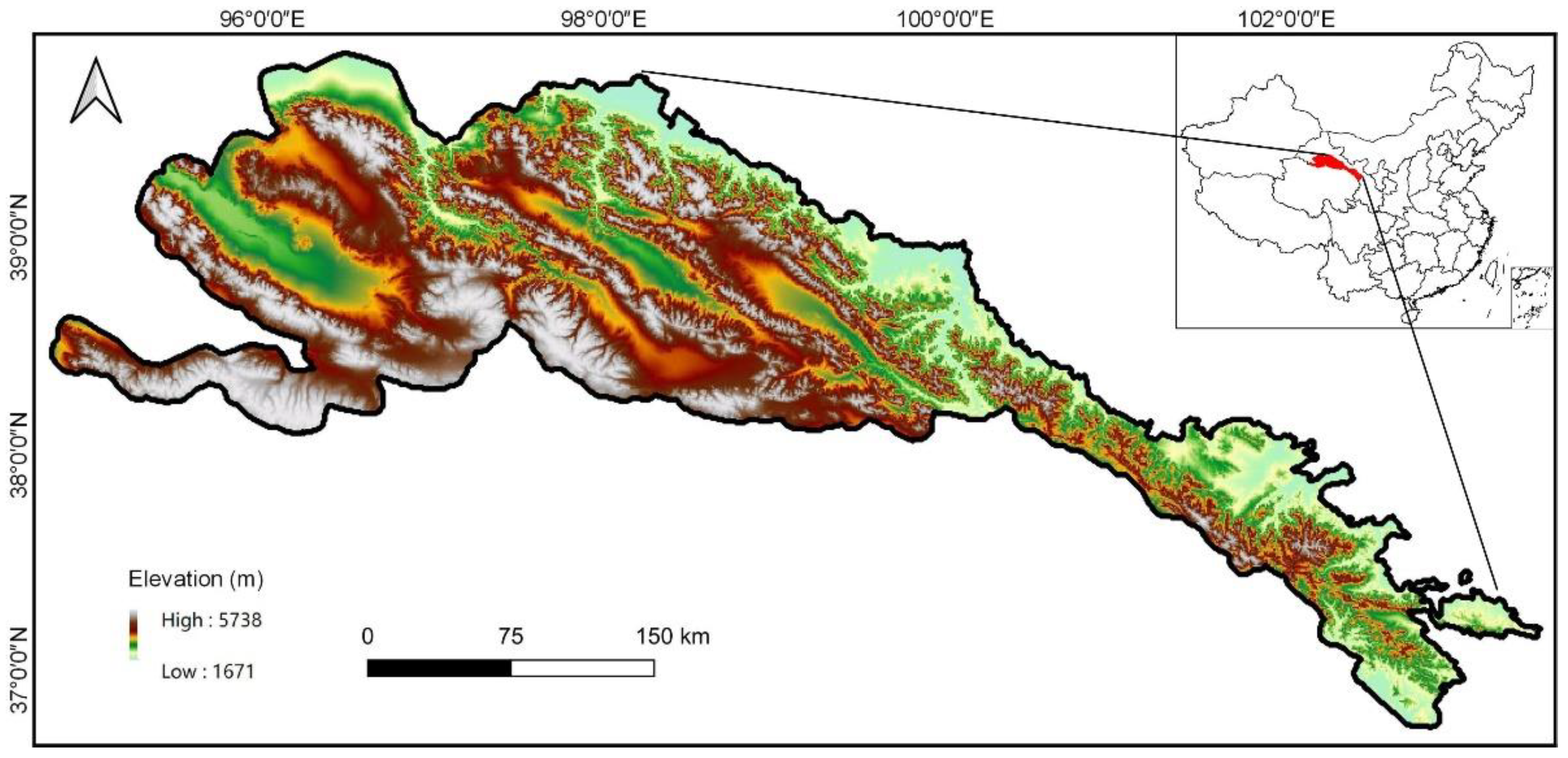
The Qilian Mountains are located in the center of Eurasia and on the northeastern margin of the Qinghai-Tibet Plateau (94°40′–103°34′E, 36°12′–40°22′N) (Figure 2), with a total area of 114,538 km2. The elevation ranges from 1671 m to 5738 m, and the terrain is high in the mountainous area and low in the plain. The Qilian Mountains are typical temperate continental and plateau climates [35]. The temperature and precipitation conditions in the Qilian Mountains vary significantly with the topography. The mean annual temperature is about 0.47 °C, and the mean annual precipitation is 36-576 mm. The main land-cover classes include forest, grassland, and shrubland.
2.2. Data Sources
The detailed data used in this study are summarized in Table 1.
2.2.1. Sentinel Imagery
The Sentinel-1 and Sentinel-2 data in 2021 were used as the main data source for forest classification. The two types of Sentinel data were acquired from the Google Earth Engine (GEE) platform and processed. The Sentinel-1 Synthetic Aperture Radar (SAR) imagery used contains one single co-polarization band of vertical transmit/vertical receive (VV) and one dual-band cross-polarization band of vertical transmit/horizontal receive (VH). Each Sentinel-1 Ground Range Detected (GRD) scene was pre-processed with the Sentinel-1 Toolbox using steps including thermal noise removal, radiometric calibration, and terrain correction. As for the Sentinel-2 multi-spectral imagery (MSI), the Level-2A orthorectified atmospherically corrected Surface Reflectance (SR) was computed with sen2cor. We first filtered the whole-year archive with the percentage of cloudy pixels less than 20%. The quality assessment (QA) band, QA60 bitmask, was then adopted to mask clouds. The 10-m bands, including blue, green, red, and near-infrared (NIR), and the 20-m bands, including red edge and shortwave infrared (SWIR), were used for further analysis. Overall, we leveraged 641 Sentinel-1 images and 902 Sentinel-2 images in this study (Tables S1 and S2).
2.2.2. Google Earth Images
Google Earth images were used as reference data for sample collection. This dataset is a seamless mosaic product of multiple satellite images. It covers historical images at multiple collection dates and zoom levels. Its highest spatial resolution can reach <1 m. We can distinguish samples more accurately with detailed information from a very high spatial resolution Google Earth image.
2.2.3. Elevation Data
The 30-m void-filled Shuttle Radar Topography Mission (SRTM) digital elevation model (DEM) data [36] on GEE was used to aid forest classification, sample interpretation, and landscape pattern analysis. It can reflect topographic features which are crucial to the subsequent analysis. The acquisition time of National Aeronautics and Space Administration (NASA) SRTM DEM data is 2000, and we suppose the terrain has been relatively stable over the years.
2.2.4. Land-Cover Products
Some other publicly available land-cover products that reflect relatively recent forest status were used for intercomparison with our forest mapping result. The products include the Finer Resolution Observation and Monitoring of Global Land Cover 10-m product (FROM-GLC10) in 2017 [37], the European Space Agency (ESA) 10-m WorldCover product in 2020 (ESA10) [38], the Esri 10-m Land Cover map in 2020 (ESRI10) [39], global 30-m land-cover product in 2020 (Globeland30) [40], the European Space Agency Climate Change Initiative (ESACCI) 300-m land-cover product in 2020 [41], and the MODIS 500-m Land Cover Type (MLCT) product in 2016 [42].
2.2.5. Climate and Human Disturbance Data
The climate and human disturbance data were used to analyze potential environmental drivers of the forest landscape pattern. The climate data, WorldClim data [43], consist of ~1-km spatial resolution monthly climate data for global land areas aggregated across a temporal range of 1970–2000. It was created by spatially interpolating weather-station data using the thin-plate splines method. The human disturbance data, Global Human Modification (gHM) of Terrestrial Systems data [44], provide a cumulative measure of human modification of terrestrial land. It was produced based on modeling the physical extent of 13 anthropogenic stressors and their estimated impacts using ~1-km spatially explicit global datasets with the median year of 2016.
2.3. Forest-Cover Mapping
2.3.1. Feature Construction
We constructed features to distinguish forest cover as listed in Table 2. In addition to the original band from Sentinel data, we calculated four widely-used indexes, including normalized difference vegetation index (NDVI) [45], enhanced vegetation index (EVI) [46], modified normalized difference water index (MNDWI) [47], and normalized difference built-up index (NDBI) [48]. The 0, 10, 25, 50, 75, 90 and 100th percentiles of each band and index were calculated to represent simplified time-series information [49]. For Sentinel-1 SAR imagery, the mean values of VV and VH polarizations were also calculated to reflect the height information. For Sentinel-2 MSI, we further used the maximum NDVI values to derive the greenest spectral composite. Other auxiliary features include geographic features (latitude and longitude) and a topographic feature (elevation).
2.3.2. Classification System
A two-level forest classification system was used in this study to reduce the impact of other land-cover types on forest classification. The level-1 classes were divided into forest and non-forest. Following the International Geosphere-Biosphere Project (IGBP) classification system [50], the forest was further divided into four level-2 classes: deciduous broadleaf forest, evergreen needleleaf forest, deciduous needleleaf forest, and mixed forest. Specifically, ‘forest’ referred to land with a tree canopy cover of more than 60 percent, and trees were defined as vegetation taller than 2 m in height.
2.3.3. Sample Collection
The sample points were randomly generated in an equal-area (300-km2) hexagonal grid. The study area was split into 487 hexagons (Figure 3). In each hexagon, 5 sample points were first generated randomly. We then supplemented 10 random sample points into each hexagon that contained forest samples to increase the number of forest samples. Google Earth images, Sentinel images, and SRTM DEM data were used for sample interpretation. Following the scheme in [51], the samples were double-checked to ensure quality. A total of 3765 samples with high reliability were collected within the study area, of which 669 samples were interpreted as forest and 3096 samples as non-forest. The forest sample points were further expanded considering the balance of forest classes. Finally, we collected 207 deciduous broadleaf forest samples, 630 evergreen needleleaf forest samples, 99 deciduous needleleaf forest samples, and 162 mixed forest samples.
2.3.4. Classification and Post-Processing
We trained the classifiers using the automated machine learning (AutoML) strategy. The AutoGluon tool [52] was applied to automate classifier selection, hyperparameter tuning, and classifier ensembling. The base classifiers include k-nearest neighbors, Light Gradient Boosting Machine (LightGBM), random forests, extremely randomized trees, CatBoost, XGBoost, and neural networks. These classifiers were trained utilizing bagging and multi-layer stack ensembling to improve classification accuracy. The number of folds used for bagging was 5. The indicator for classifier training performance was overall accuracy. The parameter ‘presets’ was set to ‘best_quality’ to get the most accurate overall classifier. The other parameters of base classifiers were initialized with default values and optimized. Specifically, in the k-nearest neighbors, the weight was set to distance. For LightGBM, the number of iterations was 10,000, the learning rate was 0.05, and the boosting type was set to the traditional Gradient Boosting Decision Tree. In random forests and extremely randomized trees, the number of trees was 300, and the criterion was set to gini. For CatBoost and XGBoost, the number of iterations was 10,000, and the learning rate was 0.05. In neural networks, the epoch was set to 30, the batch size was 256, and the base and target learning rates were 0.01 and 0.1, respectively. Classification results were then post-processed using spatial mode filtering with a 3 × 3 kernel to reduce the salt and pepper noises.
2.3.5. Accuracy Assessment and Data Intercomparison
The collected samples were randomly split into two parts, where 70% were for training, and the remaining 30% were for testing. Accuracy assessment indicators include overall accuracy, kappa coefficient [53], user’s accuracy, producer’s accuracy, F1 score, and weighted F1 score. According to the testing accuracy and running time, different classifiers were evaluated. Based on the mean decrease in the testing accuracy, the feature’s importance to the classifier was quantified. We removed features with negative importance in the final classifier to reduce redundancy and improve performance. To better reflect the classification quality, we intercompared our mapping result with other land-cover products, including FROM-GLC10, ESA10, ESRI10, Globeland30, ESACCI, and MLCT. To facilitate the comparison, we remapped these products to forest/non-forest maps referring to the class relationships in [24,49].
2.4. Landscape Pattern Analysis
To characterize the forest distribution and fragmentation pattern, we calculated several typical landscape metrics based on our forest-mapping results in Fragstats [54], including the percentage of landscape (Occupancy), patch density (PD), edge density (ED), mean patch size (MPS), mean Euclidean nearest neighbor distance (ENN), clumpiness index (Clumpy), percentage of like adjacencies (PLADJ) and patch-cohesion index (Cohesion). Considering the similarity of landscape metrics, we calculated the Pearson correlation coefficient between every two metrics. We retained those with better performance for highly correlated metrics in the subsequent regression analysis. The left metrics included Occupancy, MPS, and Cohesion (Table 3). Occupancy represents the percentage of the landscape comprised of forest, which measures landscape composition. MPS is the mean forest patch size in the landscape, a simple measure of the extent of forest fragmentation. Cohesion increases when forest patches are more clumped or aggregated in distribution, measuring the physical connectedness of the forest. The analysis was conducted within a 1 km × 1 km grid.
We used random forest regression to investigate the relationships between forest landscape metrics and environmental variables. The random forest method has the flexibility to handle complex, high-dimensional interactions, which allows it to discover relationships that are hidden in traditional parametric analysis and are unlikely to be proposed a priori by a non-omniscient observer [55]. We developed a random forest regression model for each landscape metric with environmental factors (Table 4), including climate, topography, and human disturbance factors, as independent variables. The number of trees was set to 500. The climate factors consist of mean annual temperature (MAT) and mean annual precipitation (MAP) derived from WorldClim data. The topography factors were calculated with SRTM DEM data, represented by slope, cosine of aspect (aspectCos), and relief. The aspectCos variable decreases when the aspect is near the south direction, and the relief variable indicates the degree of terrain relief within the local range. The human disturbance factor, humanModification, represents the proportion of landscape modified by anthropogenic stressors and impacts. The relative importance of each environmental variable was reflected with the Gini importance indicator. Furthermore, the marginal responses of the forest landscape metrics to important environmental variables were illustrated using partial dependence plots. Besides this, the performance () of random forest regression models was evaluated with the out-of-bag data.
3. Results
3.1. Optimal Classifier and Feature for Forest Classification
The comparison result of classifiers (Table 5) showed that the multi-layer stack ensembling strategy did help improve the performance in forest classification. In general, the ensemble learning classifier outperformed base classifiers such as random forest and CatBoost. For instance, the ensemble learning classifier achieved a 5.62% gain in the overall accuracy over the k-nearest neighbors base classifier. Meanwhile, the classifiers at the high stack level generally yielded higher accuracies than those at the low stack level. For example, the overall accuracy was improved from 91.73% to 95.20% when we increased the extremely randomized trees base classifier from the first stack level to the second stack level. However, there was an exception where the overall accuracy of the ensemble learning classifier in the second stack level (94.97%) was slightly lower than that of the XGBoost base classifier in the first stack level (95.08%). Regarding efficiency, the neural network base classifier consumed the longest marginal training time (2585 s) and prediction time (32 s), whereas it yielded a relatively lower accuracy than other base classifiers such as LightGBM and XGBoost. Overall, the multi-layer stack ensembling classifier achieved the best accuracy in terms of overall accuracy (95.44%), kappa coefficient (0.8366), and weighted F1 score (95.35%). Therefore, we chose the ensemble learning classifier as the optimal classifier for subsequent analysis.
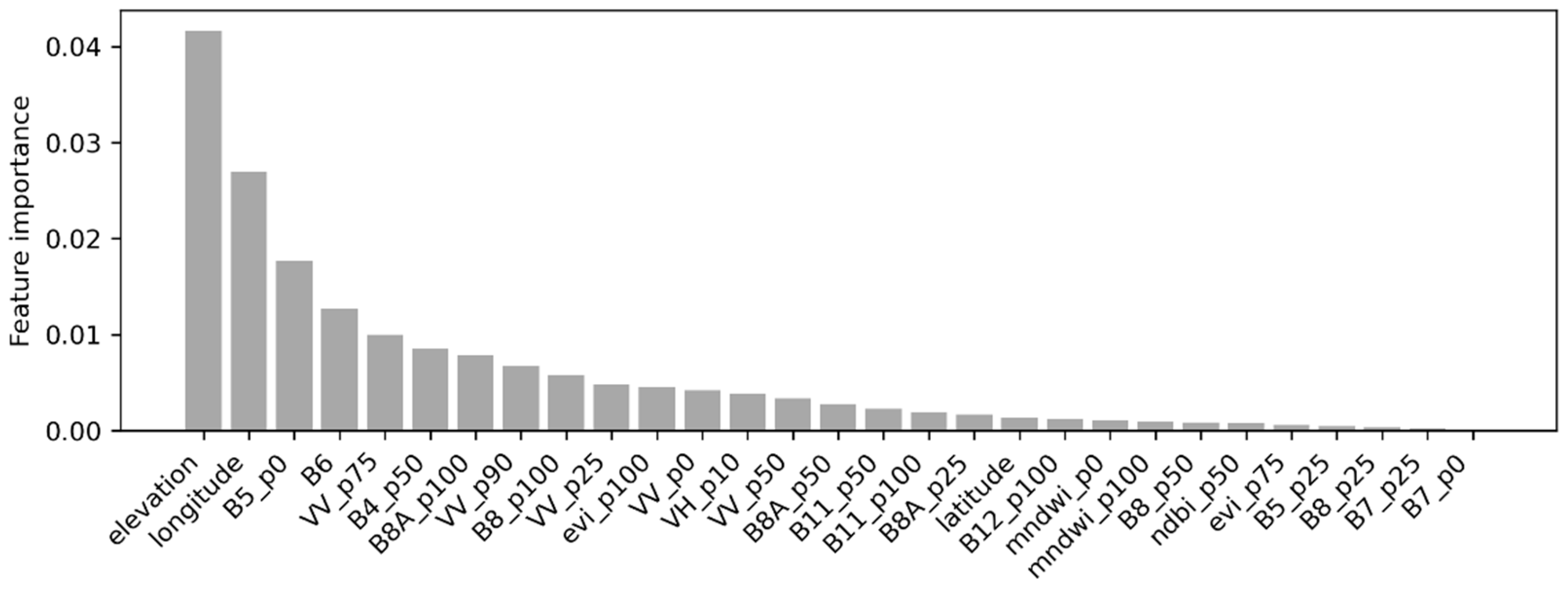
According to the feature importance (Figure 4), a total of 29 multi-dimensional features were applied in the final classifier, illustrating the usefulness of integrating multi-source information. Elevation and longitude were the leading features for forest classification, implying that the vertical and longitudinal zonality of forest distribution was crucial. Among spectral bands, the importance of red edge (B5, B6, B8A), red (B4), and NIR (B8) bands was relatively high, indicating that forests could be differentiated most in these corresponding spectral ranges. Meanwhile, EVI was the most effective spectral index for forest classification compared with other indexes such as NDVI. Besides, VV and VH polarizations also made significant contributions to forest classification. It makes sense that the SAR data help distinguish forests since they are sensitive to the geometric characteristics of the ground objects. Moreover, percentile features occupied 25 out of all the 29 features, confirming that multi-temporal information was essential in forest identification.
3.2. Reliability of Forest Mapping Result
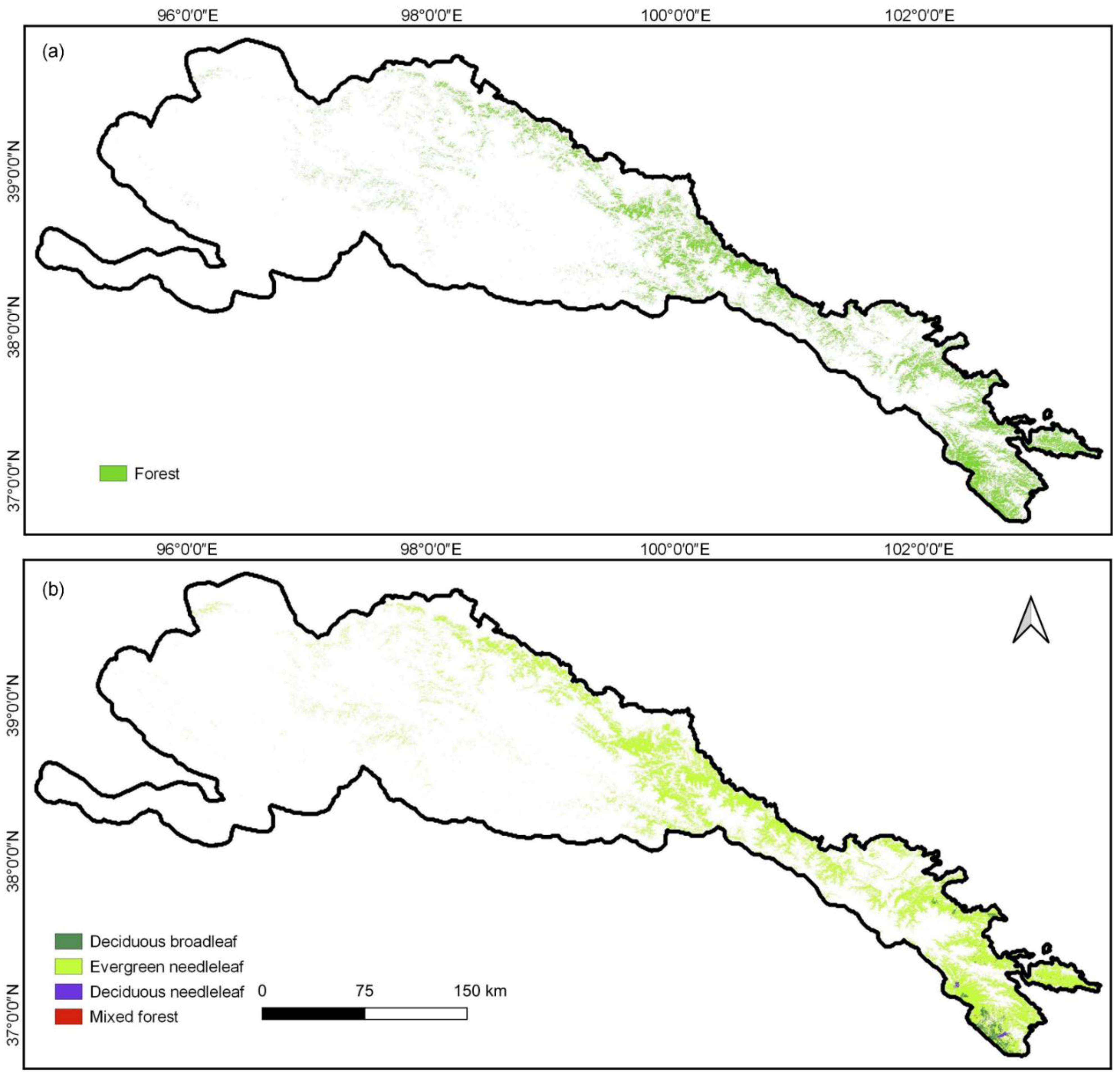
The obtained forest-mapping result across Qilian Mountains (Figure 5) was validated using test samples. The confusion matrices were calculated to evaluate accuracies. As reported in Table 6, the overall accuracy, kappa coefficient, and weighted F1 score of the level-1 forest/non-forest map reached 95.49%, 0.8384, and 95.38%, respectively, which proved the effectiveness of the overall mapping framework. The producer’s accuracy of the forest class was 81.59%, while the user’s accuracy of the forest class was 92.13%, indicating that the area of forests may be slightly underestimated. The accuracy for the non-forest class was relatively high, where both the producer’s accuracy and user’s accuracy were over 96%. In terms of the level-2 forest-cover-mapping result (Table 7), the overall accuracy, kappa coefficient, and weighted F1 score reached 78.05%, 0.6593, and 78.81%, respectively, further confirming the reliability of the proposed forest-mapping framework. Specifically, the F1 scores of deciduous broadleaf, evergreen needleleaf, deciduous needleleaf, and mixed forest class were 71.76%, 85.30%, 65.67%, and 70.27%, respectively. Among them, the identification of evergreen needleleaf forest was better than other forest classes, which may be related to the lower distribution of other forest classes (Figure 5).
Comparison results with other land-cover products further demonstrated the quality of our forest map. Quantitative accuracies with the test samples are listed in Table 8. The overall accuracy of FROM-GLC10, ESA10, ESRI10, Globeland30, ESACCI, and MLCT was 93.37%, 91.86%, 92.58%, 88.32%, 87.88%, and 83.45%, respectively. In contrast, ours was 95.49%, 2.12–12.04% higher than these other products. With the kappa coefficient or weighted F1 score as the indicator, the accuracy gap also existed or even expanded. Comparison results in selected locations are visualized in Figure 6. Among all products, ESA10, ESACCI, and MLCT could hardly identify the forest distribution, while GlobeLand30 and ESRI10 provided relatively poor spatial details of the forest. FROM-GLC10 depicted a forest pattern similar to our mapping result but slightly overestimated the forest areas. In contrast, our mapping result was more reasonable and richer in detail. Although class definitions, mapping methods, and data sources vary among products, our forest mapping results showed the best visual correspondence with Google Earth images.
3.3. Environmental Determents of Forest Landscape Pattern
The forest patch distribution in Qilian Mountains revealed certain selectivity and preference regarding geographic and topographic habitats (Figure 7). It can be seen that the forests were mainly concentrated in the eastern regions. Correspondingly, the forests were rare and scattered in the western regions, covered mainly by short vegetation or permanent snow. The forest landscape pattern was also closely related to the elevation gradient. Occupancy, MPS, and Cohesion of forests reached peak values near 3000 m. As the elevation increased or decreased, the forest landscape metrics gradually decreased. Generally, the forests were most densely distributed in regions with low-to-medium elevations ranging from 2500 m to 3500 m. In addition, the distribution of forests showed a preference for the aspect. As illustrated in Figure 7, when the north aspect with positive aspectCos values was compared, the forest patches depicted a lower occupancy and higher fragmentation degree (low MPS and Cohesion) in the south aspect with negative aspectCos values.
The random forest regression models for the forest landscape pattern performed well generally. The of models for Occupancy, MPS, and Cohesion based on out-of-bag data reached 0.91, 0.80, and 0.85, respectively. In terms of the relative importance of environmental factors (Figure 8), the three models of landscape metrics showed high consistency. The top important variables were MAT and MAP, demonstrating that the climate factor was the critical determent of the forest landscape pattern in the Qilian Mountains. Simultaneously, the importance of MAT was higher than that of MAP, indicating a stronger influence from the temperature conditions. The terrain relief made the third important contribution to the forest landscape pattern, whereas other local scale topographic variables (slope and aspectCos) showed relatively limited influence in the models. Similarly, human disturbance, represented by humanModification, did not reveal a prominent impact.
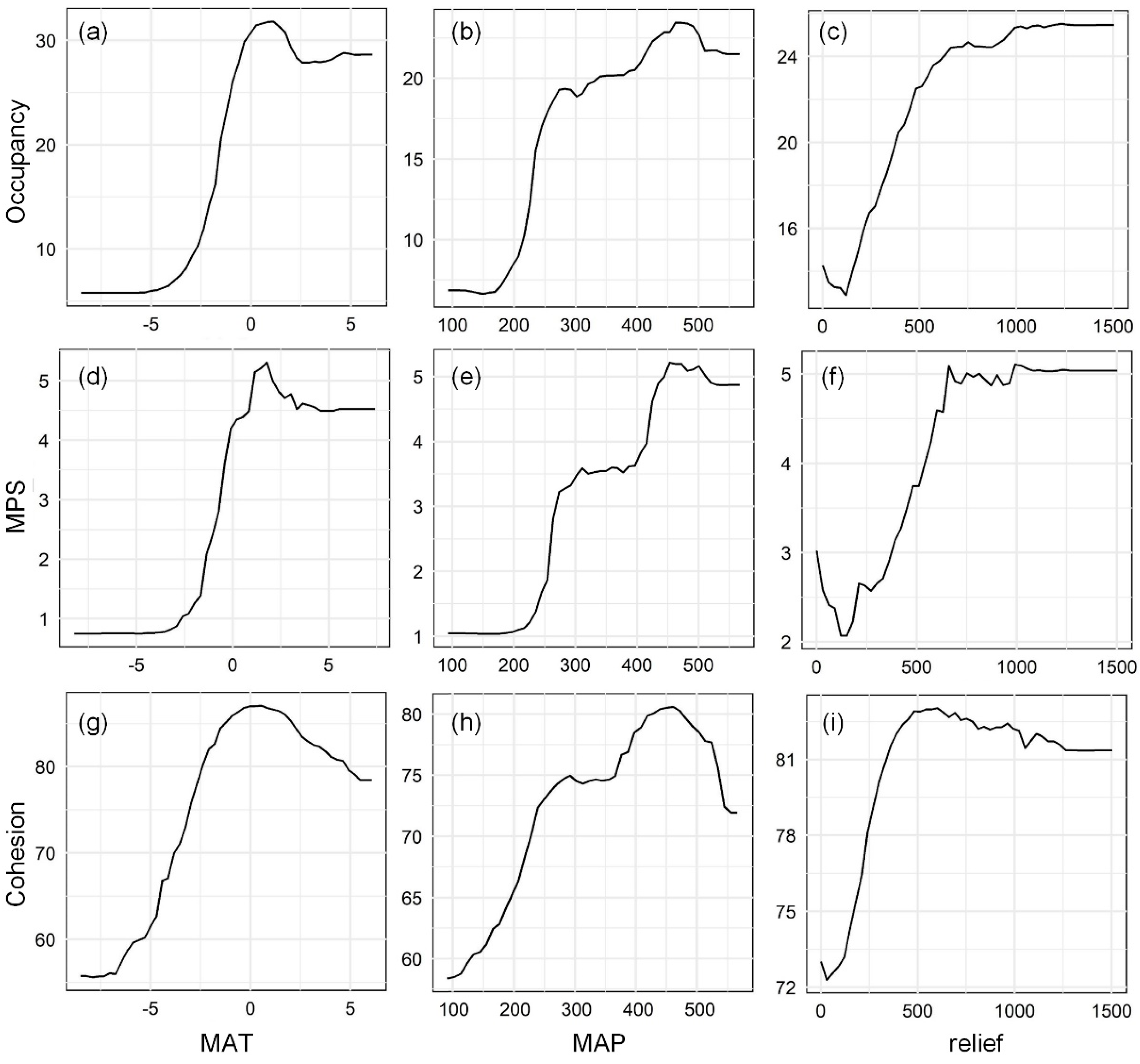
The marginal response curves of forest landscape metrics to the top three environmental variables were drawn in Figure 9. With MAT increasing, the forest landscape metrics showed approximately three-stage responses. The MAT of −5 °C, acted as a threshold, below which Occupancy, MPS, and Cohesion stayed as low as 6%, 0.8 ha, and 61%, respectively, then forest landscape metrics grew almost linearly with increasing MAT until another threshold value of about 1 °C, above which the three metrics declined from 30%, 5.2 ha, and 86%, respectively. The forest landscape metrics showed similar response curves to MAP, with a fluctuant increase as MAP increased from 100 mm to 450 mm and a slight decline as MAP reached over 450 mm. Moreover, the forest landscape metrics showed roughly increasing responses to the terrain relief from 0 m to 500 m. When the terrain relief was above 500 m, Occupancy, MPS, and Cohesion gradually stabilized at about 25%, 5 ha, and 82%.
4. Discussion
In this study, we proposed a forest classification framework based on an automated ensemble learning approach. Compared with the human–computer interaction method, machine learning algorithms showed good performance in terms of efficiency and accuracy in forest classification research [56]. The AutoML strategy can further improve classification efficiency by automating the classifier construction process. Specifically, we applied an automated ensemble machine learning strategy in leveraging a group of machine learning algorithms for forest classification. We also conducted multi-classifier and multi-feature performance comparisons, providing potential guidance for model and feature selection in forest-mapping practices. Experimental results demonstrated that ensemble learning (multi-layer stack ensembling classifier) achieved satisfactory classification accuracy, despite requiring more training time. Meanwhile, it highlights the trade-off between classification accuracy and computational cost in ensemble learning. For particular research and application needs, the balance between the accuracy and cost can be further achieved by adjusting parameters such as the target accuracy level and training time limit. In addition, comparison results among multiple land-cover products showed that our forest map was rich in detail and had higher accuracy. It further reflects the effectiveness and potential of the adopted automated ensemble machine learning framework to improve the forest mapping quality. Although deep learning algorithms with high-level representation capability have outperformed shallow machine learning techniques in some recent forest classification studies [18,22], we leveraged the latter in this study. On the one hand, the interpretability of deep learning algorithms is challenging. On the other hand, deep learning algorithms are more suitable for the information mining of very high-spatial-resolution remote sensing images. In contrast, the automated ensemble machine learning approach proved robust and cost-effective. Furthermore, the interpretability of variable importance can provide insights into the optimal choice of features in forest mapping.
A scheme of forest landscape pattern evaluation based on forest mapping data was also presented in this study. Unlike the data-acquisition method based on field surveys, remote sensing provides an unprecedented perspective on forest cover and patterns, allowing continuous maps to be constructed and spatiotemporal patterns of forest landscape to be analyzed [30]. The high-precision forest map developed based on remote sensing images can be a potential high-quality, low-cost data source for ecological and other related research. Simultaneously, the scheme of forest landscape pattern analysis based on the forest map can provide a reference for related research. Generally, the current use and interpretation of landscape metrics are constrained by the challenges of choosing a parsimonious suite of metrics for a particular application, given the plethora of existing metrics [57,58,59]. In this study, by comparing the similarity and complementarity of multiple landscape metrics, we obtained three metrics (including Occupancy, MPS, and Cohesion) with relatively strong sensitivity and characterization capacity to reflect forest distribution and landscape patterns. This can provide potential guidance for choosing metrics in other related studies. In addition, based on the forest landscape pattern, we further analyzed the driving effects of factors such as climate, topography, and human disturbance, which can help to understand the environment and conditions suitable for continuous forest distribution. The analysis results revealed that the forests in Qilian Mountains tend to be distributed in a relatively warm and humid environment. Our findings emphasized the critical role of the climatic factor in the forest landscape, which may carry implications for the protection and sustainable management of forests in the context of climate change.
However, some limitations and difficulties are still expected to be explored in future research. First, compared to the pixel-based method, the object-based method can aggregate a group of pixels together as an object, facilitating integration to form stronger features and information. In some land-cover classification studies, the object-based method improved accuracy and reduced noise [60]. Forests are also suitable for identification as patches. However, the parameter setting of the object segmentation method is a significant challenge. In this study, we used the pixel-based method to maintain rich details in the forest-mapping results. In future research, object-based forest classification optimization in areas with low local accuracies is worth attempting. Second, the obtained forest-cover map based on single-year remote sensing images is insufficient to provide richer information. On the one hand, future work should focus on classifying forest types or tree species with more classes to obtain more detailed results [61]. On the other hand, dynamic forest data are urgently needed to monitor forest status (such as forest degradation, loss, and restoration) and understand forest responses to natural disturbance and extreme weather events [62]. Third, the uncertainty in the results of forest landscape pattern analysis due to misclassification and mixed pixels should be acknowledged. Although the automated ensemble learning framework provided high-precision forest-mapping results, some classification errors still exist, which may cause certain deviations in the distribution of forest patches. Meanwhile, due to limitations in spatial resolution and spectral heterogeneity, mixed pixels may also interfere with forest landscape analysis [63]. In addition, with Sentinel data of 10-m spatial resolution, it is still difficult to capture small, highly fragmented forest patches. To tackle the issue, the forest-mapping framework should be further improved, probably using finer-spatial-resolution remote sensing images and a subpixel unmixing method in future works.
5. Conclusions
Timely and accurate forest information is critical for many scientific applications, yet forest-cover classification over mountainous areas remains challenging. In this study, leveraging multi-source remote sensing data (Sentinel-1, Sentinel-2) and automated ensemble learning algorithms, we developed a robust and cost-effective framework for forest-cover mapping. Based on this framework, we achieved high-precision and refined identification of forest cover in the Qilian Mountains. The results showed that ensemble learning was relatively robust and performed better than other base classifiers including k-nearest neighbors, LightGBM, random forests, extremely randomized trees, CatBoost, XGBoost, and neural networks. In addition to topographic and geographic information, the percentile spectral reflectance and SAR features were essential in forest cover classification. The overall accuracy of the level-1 and level-2 forest-cover maps produced reached 95.49% and 78.05%, respectively. Compared to other land-cover products, our mapping result was rich in detail and had good quality. These results elucidated the robustness and reliability of the developed framework in forest classification and demonstrated the potential and prospect of applying the framework on larger scales.
In addition, the forest landscape and fragmentation process can impact the ecosystem functions and services. However, few studies have explored the forest landscape pattern or its driving factors in ecologically fragile mountainous areas. In this context, combined with landscape metrics (Occupancy, MPS, and Cohesion) and the random forest regression method, we also designed an evaluation scheme for the forest landscape pattern and its influencing factors. Based on this scheme, we also found that the distribution of forest patches in the Qilian Mountains revealed certain selectivity and preference regarding geographic and topographical habitats. Forests were most densely distributed in the eastern regions with low-to-medium elevations and shady aspects. The regression models with climate, topography, and human disturbance factors explained 85–91% of the forest landscape pattern. Among them, climate was the critical environmental determent in the Qilian Mountains. Specifically, the top three environmental variables included MAT, MAP, and terrain relief. These findings, along with the forest mapping result, can support regional forest protection and ecological assessment, and provide implications for natural resource management and ecological restoration.
Supplementary Materials
The following supporting information can be downloaded at: https://0-www-mdpi-com.brum.beds.ac.uk/article/10.3390/rs14215470/s1, Table S1: List of Sentinel-2 images used in this study, Table S2: List of Sentinel-1 images used in this study.
Author Contributions
Conceptualization, Y.W. and H.L.; methodology, Y.W. and H.L.; software, Y.W. and H.L.; validation, Y.W. and H.L.; formal analysis, Y.W. and H.L.; investigation, Y.W. and H.L.; resources, Y.W. and H.L.; data curation, Y.W. and H.L.; writing—original draft preparation, Y.W. and H.L.; writing—review and editing, Y.W., H.L., L.S. and J.W.; visualization, Y.W. and H.L.; supervision, H.L.; project administration, H.L. and L.S.; funding acquisition, H.L. and L.S. All authors have read and agreed to the published version of the manuscript.
Funding
This research was funded by the National Key Research and Development Program of China (2021YFD1500204) and Open Research Fund Program of Key Laboratory of Digital Mapping and Land Information Application, Minisitry of Natural Resources (ZRZYBWD202210).
Data Availability Statement
Not applicable.
Conflicts of Interest
The authors declare no conflict of interest.
References
- Hansen, M.C.; Potapov, P.V.; Moore, R.; Hancher, M.; Turubanova, S.A.; Tyukavina, A.; Thau, D.; Stehman, S.V.; Goetz, S.J.; Loveland, T.R.; et al. High-Resolution Global Maps of 21st-century Forest Cover Change. Science 2013, 342, 850. [Google Scholar] [CrossRef] [PubMed] [Green Version]
- Harris, N.L.; Gibbs, D.A.; Baccini, A.; Birdsey, R.A.; de Bruin, S.; Farina, M.; Fatoyinbo, L.; Hansen, M.C.; Herold, M.; Houghton, R.A.; et al. Global Maps of Twenty-First Century Forest Carbon Fluxes. Nat. Clim. Chang. 2021, 11, 234–240. [Google Scholar] [CrossRef]
- FAO; UNEP. The State of the World’s Forests 2020. Forests, Biodiversity and People; Reports; FAO: Rome, Italy, 2020; pp. 10–15. [Google Scholar] [CrossRef]
- Bonan, G.B. Forests and Climate Change: Forcings, Feedbacks, and the Climate Benefits of Forests. Science 2008, 320, 1444–1449. [Google Scholar] [CrossRef] [PubMed] [Green Version]
- Chazdon Robin, L. Beyond Deforestation: Restoring Forests and Ecosystem Services on Degraded Lands. Science 2008, 320, 1458–1460. [Google Scholar] [CrossRef] [PubMed] [Green Version]
- Scheffer, M.; Carpenter, S.; Foley, J.A.; Folke, C.; Walker, B. Catastrophic Shifts in Ecosystems. Nature 2001, 413, 591–596. [Google Scholar] [CrossRef]
- Qin, Y.; Xiao, X.; Wigneron, J.-P.; Ciais, P.; Brandt, M.; Fan, L.; Li, X.; Crowell, S.; Wu, X.; Doughty, R.; et al. Carbon Loss from Forest Degradation Exceeds that from Deforestation in the Brazilian Amazon. Nat. Clim. Chang. 2021, 11, 442–448. [Google Scholar] [CrossRef]
- EEA. High Resolution Layer: Forest Type (FTY). 2015. Available online: https://land.copernicus.eu/pan-european/high-resolution-layers/forests/forest-type-1/status-maps/2015?tab=metadata (accessed on 27 August 2022).
- EEA. High Resolution Layer Forest, Dominant Leaf Type. 2018. Available online: https://land.copernicus.eu/pan-european/high-resolution-layers/forests/dominant-leaf-type/status-maps/dominant-leaf-type-2018 (accessed on 27 August 2022).
- Ma, M.; Liu, J.; Liu, M.; Zeng, J.; Li, Y. Tree Species Classification Based on Sentinel-2 Imagery and Random Forest Classifier in the Eastern Regions of the Qilian Mountains. Forests 2021, 12, 1736. [Google Scholar] [CrossRef]
- Hemmerling, J.; Pflugmacher, D.; Hostert, P. Mapping Temperate Forest Tree Species Using Dense Sentinel-2 Time Series. Remote Sens. Environ. 2021, 267, 112743. [Google Scholar] [CrossRef]
- Hamrouni, Y.; Paillassa, E.; Chéret, V.; Monteil, C.; Sheeren, D. Sentinel-2 Poplar Index for Operational Mapping of Poplar Plantations over Large Areas. Remote Sens. 2022, 14, 3975. [Google Scholar] [CrossRef]
- Yu, H.; Ni, W.; Zhang, Z.; Sun, G.; Zhang, Z. Regional Forest Mapping over Mountainous Areas in Northeast China Using Newly Identified Critical Temporal Features of Sentinel-1 Backscattering. Remote Sens. 2020, 12, 1485. [Google Scholar] [CrossRef]
- Dostálová, A.; Lang, M.; Ivanovs, J.; Waser, L.T.; Wagner, W. European Wide Forest Classification Based on Sentinel-1 Data. Remote Sens. 2021, 13, 337. [Google Scholar] [CrossRef]
- De Luca, G.; MN Silva, J.; Di Fazio, S.; Modica, G. Integrated Use of Sentinel-1 and Sentinel-2 Data and Open-Source Machine Learning Algorithms for Land Cover Mapping in a Mediterranean Region. Eur. J. Remote Sens. 2022, 55, 52–70. [Google Scholar] [CrossRef]
- Mngadi, M.; Odindi, J.; Peerbhay, K.; Mutanga, O. Examining the Effectiveness of Sentinel-1 and 2 Imagery for Commercial Forest Species Mapping. Geocarto Int. 2021, 36, 1–12. [Google Scholar] [CrossRef]
- Ghorbanian, A.; Zaghian, S.; Asiyabi, R.M.; Amani, M.; Mohammadzadeh, A.; Jamali, S. Mangrove Ecosystem Mapping Using Sentinel-1 and Sentinel-2 Satellite Images and Random Forest Algorithm in Google Earth Engine. Remote Sens. 2021, 13, 2565. [Google Scholar] [CrossRef]
- Waser, L.T.; Rüetschi, M.; Psomas, A.; Small, D.; Rehush, N. Mapping Dominant Leaf Type based on Combined Sentinel-1/-2 Data—Challenges for Mountainous Countries. ISPRS J. Photogramm. Remote Sens. 2021, 180, 209–226. [Google Scholar] [CrossRef]
- Zhang, W.; Brandt, M.; Wang, Q.; Prishchepov, A.V.; Tucker, C.J.; Li, Y.; Lyu, H.; Fensholt, R. From Woody Cover to Woody Canopies: How Sentinel-1 and Sentinel-2 Data Advance the Mapping of Woody Plants in Savannas. Remote Sens. Environ. 2019, 234, 111465. [Google Scholar] [CrossRef]
- Pulella, A.; Aragão Santos, R.; Sica, F.; Posovszky, P.; Rizzoli, P. Multi-Temporal Sentinel-1 Backscatter and Coherence for Rainforest Mapping. Remote Sens. 2020, 12, 847. [Google Scholar] [CrossRef] [Green Version]
- Chen, L.; Tian, X.; Chai, G.; Zhang, X.; Chen, E. A New CBAM-P-Net Model for Few-Shot Forest Species Classification Using Airborne Hyperspectral Images. Remote Sens. 2021, 13, 1269. [Google Scholar] [CrossRef]
- D’Amico, G.; Francini, S.; Giannetti, F.; Vangi, E.; Travaglini, D.; Chianucci, F.; Mattioli, W.; Grotti, M.; Puletti, N.; Corona, P.; et al. A deep learning approach for automatic mapping of poplar plantations using Sentinel-2 imagery. GIScience Remote Sens. 2021, 58, 1352–1368. [Google Scholar] [CrossRef]
- Liu, H.; Li, J.; He, L.; Wang, Y. Superpixel-Guided Layer-Wise Embedding CNN for Remote Sensing Image Classification. Remote Sens. 2019, 11, 174. [Google Scholar] [CrossRef] [Green Version]
- Liu, H.; Gong, P.; Wang, J.; Wang, X.; Ning, G.; Xu, B. Production of Global Daily Seamless Data Cubes and Quantification of Global Land Cover Change from 1985 to 2020-iMap World 1.0. Remote Sens. Environ. 2021, 258, 112364. [Google Scholar] [CrossRef]
- Grabska, E.; Frantz, D.; Ostapowicz, K. Evaluation of Machine Learning Algorithms for Forest Stand Species Mapping Using Sentinel-2 Imagery and Environmental Data in the Polish Carpathians. Remote Sens. Environ. 2020, 251, 112103. [Google Scholar] [CrossRef]
- Fahrig, L. Habitat Fragmentation: A Long and Tangled Tale. Glob. Ecol. Biogeogr. 2019, 28, 33–41. [Google Scholar] [CrossRef]
- Brinck, K.; Fischer, R.; Groeneveld, J.; Lehmann, S.; Dantas De Paula, M.; Pütz, S.; Sexton, J.O.; Song, D.; Huth, A. High Resolution Analysis of Tropical Forest Fragmentation and Its Impact on the Global Carbon Cycle. Nat. Commun. 2017, 8, 14855. [Google Scholar] [CrossRef] [Green Version]
- Haddad Nick, M.; Brudvig Lars, A.; Clobert, J.; Davies Kendi, F.; Gonzalez, A.; Holt Robert, D.; Lovejoy Thomas, E.; Sexton Joseph, O.; Austin Mike, P.; Collins Cathy, D.; et al. Habitat Fragmentation and Its Lasting Impact on Earth’s Ecosystems. Sci. Adv. 2015, 1, e1500052. [Google Scholar] [CrossRef] [Green Version]
- Potapov, P.; Hansen Matthew, C.; Laestadius, L.; Turubanova, S.; Yaroshenko, A.; Thies, C.; Smith, W.; Zhuravleva, I.; Komarova, A.; Minnemeyer, S.; et al. The Last Frontiers of Wilderness: Tracking Loss of Intact Forest Landscapes from 2000 to 2013. Sci. Adv. 2017, 3, e1600821. [Google Scholar] [CrossRef] [Green Version]
- Taubert, F.; Fischer, R.; Groeneveld, J.; Lehmann, S.; Müller, M.S.; Rödig, E.; Wiegand, T.; Huth, A. Global Patterns of Tropical Forest Fragmentation. Nature 2018, 554, 519–522. [Google Scholar] [CrossRef]
- Fischer, R.; Taubert, F.; Müller Michael, S.; Groeneveld, J.; Lehmann, S.; Wiegand, T.; Huth, A. Accelerated Forest Fragmentation Leads to Critical Increase in Tropical Forest Edge Area. Sci. Adv. 2021, 7, eabg7012. [Google Scholar] [CrossRef]
- Myers, N.; Mittermeier, R.A.; Mittermeier, C.G.; da Fonseca, G.A.B.; Kent, J. Biodiversity Hotspots for Conservation Priorities. Nature 2000, 403, 853–858. [Google Scholar] [CrossRef] [PubMed]
- Yang, W.; Wang, Y.; Wang, S.; Webb, A.A.; Yu, P.; Liu, X.; Zhang, X. Spatial Distribution of Qinghai Spruce Forests and the Thresholds of Influencing Factors in a Small Catchment, Qilian Mountains, Northwest China. Sci. Rep. 2017, 7, 5561. [Google Scholar] [CrossRef] [PubMed] [Green Version]
- Zongxing, L.; Qi, F.; Zongjie, L.; Xufeng, W.; Juan, G.; Baijuan, Z.; Yuchen, L.; Xiaohong, D.; Jian, X.; Wende, G.; et al. Reversing Conflict between Humans and the Environment—The Experience in the Qilian Mountains. Renew. Sustain. Energy Rev. 2021, 148, 111333. [Google Scholar] [CrossRef]
- Geng, L.; Che, T.; Wang, X.; Wang, H. Detecting Spatiotemporal Changes in Vegetation with the BFAST Model in the Qilian Mountain Region during 2000–2017. Remote Sens. 2019, 11, 103. [Google Scholar] [CrossRef] [Green Version]
- Farr, T.G.; Rosen, P.A.; Caro, E.; Crippen, R.; Duren, R.; Hensley, S.; Kobrick, M.; Paller, M.; Rodriguez, E.; Roth, L.; et al. The Shuttle Radar Topography Mission. Rev. Geophys. 2007, 45. [Google Scholar] [CrossRef] [Green Version]
- Gong, P.; Liu, H.; Zhang, M.; Li, C.; Wang, J.; Huang, H.; Clinton, N.; Ji, L.; Li, W.; Bai, Y.; et al. Stable Classification with Limited Sample: Transferring a 30-m resolution Sample Set Collected in 2015 to Mapping 10-m Resolution Global Land Cover in 2017. Sci. Bull. 2019, 64, 370–373. [Google Scholar] [CrossRef] [Green Version]
- Zanaga, D.; Van De Kerchove, R.; De Keersmaecker, W.; Souverijns, N.; Brockmann, C.; Quast, R.; Wevers, J.; Grosu, A.; Paccini, A.; Vergnaud, S.; et al. ESA WorldCover 10 m 2020 v100. 2021. Available online: https://zenodo.org/record/5571936 (accessed on 1 May 2022).
- Karra, K.; Kontgis, C.; Statman-Weil, Z.; Mazzariello, J.C.; Mathis, M.; Brumby, S.P. Global Land Use/Land Cover with Sentinel 2 and Deep Learning. In Proceedings of the 2021 IEEE International Geoscience and Remote Sensing Symposium IGARSS, Brussels, Belgium, 11–16 July 2021; pp. 4704–4707. [Google Scholar]
- Chen, J.; Chen, J.; Liao, A.; Cao, X.; Chen, L.; Chen, X.; He, C.; Han, G.; Peng, S.; Lu, M. Global Land Cover Mapping at 30 m Resolution: A POK-Based Operational Approach. ISPRS J. Photogramm. Remote Sens. 2015, 103, 7–27. [Google Scholar] [CrossRef] [Green Version]
- ESA. Land Cover CCI Product User Guide Version 2. Technical Reports. 2017. Available online: Maps.elie.ucl.ac.be/CCI/viewer/download/ESACCI-LC-Ph2-PUGv2_2.0.pdf (accessed on 1 May 2022).
- Sulla-Menashe, D.; Gray, J.M.; Abercrombie, S.P.; Friedl, M.A. Hierarchical Mapping of Annual Global Land Cover 2001 to Present: The MODIS Collection 6 Land Cover product. Remote Sens. Environ. 2019, 222, 183–194. [Google Scholar] [CrossRef]
- Fick, S.E.; Hijmans, R.J. WorldClim 2: New 1-km Spatial Resolution Climate Surfaces for Global Land Areas. Int. J. Climatol. 2017, 37, 4302–4315. [Google Scholar] [CrossRef]
- Kennedy, C.M.; Oakleaf, J.R.; Theobald, D.M.; Baruch-Mordo, S.; Kiesecker, J. Managing the Middle: A Shift in Conservation Priorities based on the Global Human Modification Gradient. Glob. Chang. Biol. 2019, 25, 811–826. [Google Scholar] [CrossRef]
- Rouse, J.; Haas, R.H.; Schell, J.A.; Deering, D.W. Monitoring Vegetation Systems in the Great Plains with ERTS. NASA Spec. Publ. 1974, 351, 309. [Google Scholar]
- Liu, H.Q.; Huete, A. A Feedback based Modification of the NDVI to Minimize Canopy Background and Atmospheric Noise. IEEE Trans. Geosci. Remote Sens. 1995, 33, 457–465. [Google Scholar] [CrossRef]
- Xu, H. Modification of Normalised Difference Water Index (NDWI) to Enhance Open Water Features in Remotely Sensed Imagery. Int. J. Remote Sens. 2006, 27, 3025–3033. [Google Scholar] [CrossRef]
- Zha, Y.; Gao, J.; Ni, S. Use of Normalized Difference Built-up Index in Automatically Mapping Urban Areas from TM Imagery. Int. J. Remote Sens. 2003, 24, 583–594. [Google Scholar] [CrossRef]
- Liu, H.; Gong, P.; Wang, J.; Clinton, N.; Bai, Y.; Liang, S. Annual Dynamics of Global Land Cover and its Long-Term Changes from 1982 to 2015. Earth Syst. Sci. Data 2020, 12, 1217–1243. [Google Scholar] [CrossRef]
- Loveland, T.R.; Reed, B.C.; Brown, J.F.; Ohlen, D.O.; Zhu, Z.; Yang, L.; Merchant, J.W. Development of a Global Land Cover Characteristics Database and IGBP DISCover from 1 km AVHRR Data. Int. J. Remote Sens. 2000, 21, 1303–1330. [Google Scholar] [CrossRef]
- Zhao, Y.; Gong, P.; Yu, L.; Hu, L.; Li, X.; Li, C.; Zhang, H.; Zheng, Y.; Wang, J.; Zhao, Y.; et al. Towards a Common Validation Sample Set for Global Land-Cover Mapping. Int. J. Remote Sens. 2014, 35, 4795–4814. [Google Scholar] [CrossRef]
- Erickson, N.; Mueller, J.; Shirkov, A.; Zhang, H.; Larroy, P.; Li, M.; Smola, A. AutoGluon-Tabular: Robust and Accurate AutoML for Structured Data. arXiv 2020, arXiv:2003.06505. [Google Scholar] [CrossRef]
- Cohen, J. A Coefficient of Agreement for Nominal Scales. Educ. Psychol. Meas. 1960, 20, 37–46. [Google Scholar] [CrossRef]
- McGarigal, K. FRAGSTATS: Spatial Pattern Analysis Program for Quantifying Landscape Structure; US Department of Agriculture, Forest Service, Pacific Northwest Research Station: Portland, ON, USA, 1995; Volume 351. [Google Scholar]
- Evans, J.S.; Murphy, M.A.; Holden, Z.A.; Cushman, S.A. Modeling Species Distribution and Change Using Random Forest. In Predictive Species and Habitat Modeling in Landscape Ecology: Concepts and Applications; Drew, C.A., Wiersma, Y.F., Huettmann, F., Eds.; Springer: New York, NY, USA, 2011; pp. 139–159. [Google Scholar]
- Verhegghen, A.; Kuzelova, K.; Syrris, V.; Eva, H.; Achard, F. Mapping Canopy Cover in African Dry Forests from the Combined Use of Sentinel-1 and Sentinel-2 Data: Application to Tanzania for the Year 2018. Remote Sens. 2022, 14, 1522. [Google Scholar] [CrossRef]
- McGarigal, K. Landscape Pattern Metrics. In Wiley StatsRef: Statistics Reference Online; Balakrishnan, N., Colton, T., Everitt, B., Piegorsch, W., Ruggeri, F., Teugels, J.L., Eds.; John Wiley & Sons, Ltd.: Hoboken, NJ, USA, 2014. [Google Scholar]
- Wang, X.; Blanchet, F.G.; Koper, N. Measuring Habitat Fragmentation: An Evaluation of Landscape Pattern Metrics. Methods Ecol. Evol. 2014, 5, 634–646. [Google Scholar] [CrossRef]
- Chambers, C.L.; Cushman, S.A.; Medina-Fitoria, A.; Martínez-Fonseca, J.; Chávez-Velásquez, M. Influences of Scale on Bat Habitat Relationships in a Forested Landscape in Nicaragua. Landsc. Ecol. 2016, 31, 1299–1318. [Google Scholar] [CrossRef]
- Martins, V.S.; Kaleita, A.L.; Gelder, B.K.; da Silveira, H.L.F.; Abe, C.A. Exploring Multiscale Object-Based Convolutional Neural Network (Multi-OCNN) for Remote Sensing Image Classification at High Spatial Resolution. ISPRS J. Photogramm. Remote Sens. 2020, 168, 56–73. [Google Scholar] [CrossRef]
- Giannetti, F.; Barbati, A.; Mancini, L.D.; Travaglini, D.; Bastrup-Birk, A.; Canullo, R.; Nocentini, S.; Chirici, G. European Forest Types: Toward an Automated Classification. Ann. For. Sci. 2018, 75, 6. [Google Scholar] [CrossRef] [Green Version]
- Liu, F.; Liu, H.; Xu, C.; Shi, L.; Zhu, X.; Qi, Y.; He, W. Old-Growth Forests Show Low Canopy Resilience to Droughts at the Southern Edge of the Taiga. Glob. Chang. Biol. 2021, 27, 2392–2402. [Google Scholar] [CrossRef] [PubMed]
- Gudex-Cross, D.; Pontius, J.; Adams, A. Enhanced Forest Cover Mapping Using Spectral Unmixing and Object-Based Classification of Multi-Temporal Landsat Imagery. Remote Sens. Environ. 2017, 196, 193–204. [Google Scholar] [CrossRef]
Figure 1.
The framework for forest mapping and landscape pattern analysis.

Figure 2.
The geographical location of the Qilian Mountains.

Figure 3.
The distribution of collected samples.

Figure 4.
The relative importance of features for forest classification. Note: the suffixes in the feature names, including p0, p10, p25, p50, p75, p90, and p100, stand for the percentile values.
Figure 4.
The relative importance of features for forest classification. Note: the suffixes in the feature names, including p0, p10, p25, p50, p75, p90, and p100, stand for the percentile values.

Figure 5.
The forest-mapping result across the Qilian Mountains in 2021. (a) the level-1 forest-cover map; (b) the level-2 forest-cover map.
Figure 5.
The forest-mapping result across the Qilian Mountains in 2021. (a) the level-1 forest-cover map; (b) the level-2 forest-cover map.

Figure 6.
Comparison of our level-1 forest mapping result, FROM-GLC10, ESA10, ESRI10, GlobeLand30, ESACCI, and MLCT in selected locations. (a) centered at 101.0°N, 38.2°E; (b) centered at 100.4°N, 38.5°E.
Figure 6.
Comparison of our level-1 forest mapping result, FROM-GLC10, ESA10, ESRI10, GlobeLand30, ESACCI, and MLCT in selected locations. (a) centered at 101.0°N, 38.2°E; (b) centered at 100.4°N, 38.5°E.

Figure 7.
The forest landscape pattern in the Qilian Mountains. (a) Occupancy; (b) mean patch size (MPS); (c) Cohesion.
Figure 7.
The forest landscape pattern in the Qilian Mountains. (a) Occupancy; (b) mean patch size (MPS); (c) Cohesion.

Figure 8.
The relative importance of environmental variables for forest landscape metrics.

Figure 9.
The marginal responses of forest landscape metrics to important environmental variables. (a) Occupancy to mean annual temperature (MAT); (b) Occupancy to mean annual precipitation (MAP); (c) Occupancy to relief; (d) mean patch size (MPS) to MAT; (e) MPS to MAP; (f) MPS to relief; (g) Cohesion to MAT; (h) Cohesion to MAP; (i) Cohesion to relief.


Table 1.
The detailed information of data used in this study.
| Category | Data Source | Spatial Resolution | Time |
|---|---|---|---|
| SAR | Sentinel-1 GRD | 10 m | 2021 |
| MSI | Sentinel-2 Level-2 SR | 10-20 m | 2021 |
| Google Earth images | Google Earth images | <1 m (highest) | 2020–2021 (most) |
| Topography | SRTM DEM | 30 m | 2000 |
| Land cover | FROM-GLC10 | 10 m | 2017 |
| ESA10 | 10 m | 2020 | |
| ESRI10 | 10 m | 2020 | |
| Globeland30 | 30 m | 2020 | |
| ESACCI | 300 m | 2020 | |
| MLCT | 500 m | 2016 | |
| Climate | WorldClim | ~1 km | 1970–2000 |
| Human disturbance | gHM | ~1 km | 2016 |
Table 2.
The explanatory table of the constructed features for forest classification.
| Data source | Band | Description | Feature |
|---|---|---|---|
| Sentinel-1 SAR | VV | Single co-polarization, vertical transmit/vertical receive | Mean values and percentiles (0, 10, 25, 50, 75, 90, and 100) |
| VH | Dual-band cross-polarization, vertical transmit/horizontal receive | ||
| Sentinel-2 MSI | B2 | Blue | Greenest composite values and percentiles (0, 10, 25, 50, 75, 90, and 100) |
| B3 | Green | ||
| B4 | Red | ||
| B5 | Red Edge 1 | ||
| B6 | Red Edge 2 | ||
| B7 | Red Edge 3 | ||
| B8 | NIR | ||
| B8A | Red Edge 4 | ||
| B11 | SWIR 1 | ||
| B12 | SWIR 2 | ||
| NDVI | (B8 − B4)/(B8 + B4) | ||
| EVI | 2.5 × (B8 − B4)/(B8 + B4 × 6 − B2 × 7.5 + 1) | ||
| MNDWI | (B3 − B11)/(B3 + B11) | ||
| NDBI | (B11 − B8)/(B11 + B8) | ||
| SRTM DEM | Elevation | ||
| Location | Longitude | ||
| Latitude | |||
Table 3.
The landscape metrics for forest pattern analysis.
| Landscape Metric | Description | Note |
|---|---|---|
| Percentage of landscape (Occupancy) | Occupancy = (100) | = number of forest patches = area of forest patch () A = total landscape area () = perimeter of forest patch (km) |
| Mean patch size (MPS) | MPS = (100) () | |
| Patch cohesion index (Cohesion) | Cohesion = (100) |
Table 4.
The environmental variables for forest landscape pattern analysis.
| Factor | Variable | Description | Data Source |
|---|---|---|---|
| Climate | MAT | Mean annual temperature (°C) | WorldClim |
| MAP | Mean annual precipitation () | ||
| Topography | slope | (°) | SRTM DEM |
| aspectCos | aspectCos = cosine(aspect) | ||
| relief | relief = (m), where and are maximum, minimum values of elevation within a 3 × 3 range, respectively. | ||
| Human disturbance | humanModification | The indicator of human modification | gHM |
Table 5.
Comparison of classifiers in terms of level-1 forest classification accuracies and running time *.
Table 5.
Comparison of classifiers in terms of level-1 forest classification accuracies and running time *.
| Classifier | Overall Accuracy | Kappa | Weighted F1 | Training Time (s) | Prediction Time (s) | Stack Level |
|---|---|---|---|---|---|---|
| WeightedEnsemble_L3 | 95.44% | 0.8366 | 95.35% | 3.1285 | 0.0023 | 3 |
| LightGBM_BAG_L2 | 95.35% | 0.8342 | 95.23% | 97.7112 | 1.5135 | 2 |
| ExtraTreesGini_BAG_L2 | 95.20% | 0.8327 | 95.19% | 1.0046 | 0.1096 | 2 |
| XGBoost_BAG_L2 | 95.15% | 0.8321 | 95.07% | 271.8431 | 6.8048 | 2 |
| RandomForestGini_BAG_L2 | 95.11% | 0.8315 | 95.07% | 6.1541 | 0.1130 | 2 |
| NeuralNetFastAI_BAG_L2 | 95.08% | 0.8302 | 95.11% | 2584.8642 | 31.8396 | 2 |
| XGBoost_BAG_L1 | 95.08% | 0.8300 | 95.06% | 568.8886 | 8.6990 | 1 |
| CatBoost_BAG_L2 | 95.03% | 0.8295 | 95.01% | 178.3345 | 0.4817 | 2 |
| WeightedEnsemble_L2 | 94.97% | 0.8288 | 94.66% | 3.8371 | 0.0058 | 2 |
| LightGBM_BAG_L1 | 94.87% | 0.8271 | 94.57% | 205.4603 | 3.7624 | 1 |
| CatBoost_BAG_L1 | 94.66% | 0.8240 | 94.41% | 456.5169 | 0.5143 | 1 |
| NeuralNetFastAI_BAG_L1 | 93.94% | 0.8184 | 93.75% | 2731.8908 | 29.8472 | 1 |
| RandomForestGini_BAG_L1 | 92.46% | 0.7906 | 92.42% | 6.5490 | 0.2591 | 1 |
| ExtraTreesGini_BAG_L1 | 91.73% | 0.7807 | 91.26% | 1.0625 | 0.1114 | 1 |
| KNeighborsDist_BAG_L1 | 89.82% | 0.7445 | 89.36% | 0.0992 | 5.3558 | 1 |
* WeightedEnsemble, LightGBM_BAG, ExtraTreesGini_BAG, XGBoost_BAG, RandomForestGini_BAG, NeuralNetFastAI_BAG, CatBoost_BAG, and KNeighborsDist_BAG represent ensemble learning, LightGBM, extremely randomized trees, XGBoost, random forests, neural networks, CatBoost, and k-nearest neighbors, respectively. The suffixes L3, L2, and L1 refer to stack levels.
Table 6.
The confusion matrix for our level-1 forest-cover map using the test samples.
| Class | Non-Forest | Forest | Producer’s Accuracy | User’s Accuracy | F1 |
|---|---|---|---|---|---|
| Non-forest | 915 | 14 | 98.49% | 96.11% | 97.29% |
| Forest | 37 | 164 | 81.59% | 92.13% | 86.54% |
| Overall accuracy = 95.49% | Kappa = 0.8384 | Weighted F1 = 95.38% | |||
Table 7.
The confusion matrix for our level-2 forest-cover map using the test samples.
| Class | Deciduous Broadleaf | Evergreen Needleleaf | Deciduous Needleleaf | Mixed Forest | Producer’s Accuracy | User’s Accuracy | F1 |
|---|---|---|---|---|---|---|---|
| Deciduous broadleaf | 47 | 6 | 4 | 5 | 75.81% | 68.12% | 71.76% |
| Evergreen needleleaf | 13 | 148 | 11 | 17 | 78.31% | 93.67% | 85.30% |
| Deciduous needleleaf | 3 | 2 | 22 | 2 | 75.86% | 57.89% | 65.67% |
| Mixed forest | 6 | 2 | 1 | 39 | 81.25% | 61.90% | 70.27% |
| Overall accuracy = 78.05% | Kappa = 0.6593 | Weighted F1 = 78.81% | |||||
Table 8.
Comparison of our mapping result, FROM-GLC10, ESA10, ESRI10, GlobeLand30, ESACCI, and MLCT in terms of accuracies.
Table 8.
Comparison of our mapping result, FROM-GLC10, ESA10, ESRI10, GlobeLand30, ESACCI, and MLCT in terms of accuracies.
| Data | Overall Accuracy | Kappa | Weighted F1 |
|---|---|---|---|
| Ours | 95.49% | 0.8384 | 95.38% |
| FROM-GLC10 | 93.37% | 0.7892 | 93.33% |
| ESA10 | 91.86% | 0.7671 | 91.96% |
| ESRI10 | 92.58% | 0.7649 | 92.51% |
| Globeland30 | 88.32% | 0.5990 | 88.30% |
| ESACCI | 87.88% | 0.4519 | 85.52% |
| MLCT | 83.45% | 0.1150 | 77.15% |
Publisher’s Note: MDPI stays neutral with regard to jurisdictional claims in published maps and institutional affiliations. |
© 2022 by the authors. Licensee MDPI, Basel, Switzerland. This article is an open access article distributed under the terms and conditions of the Creative Commons Attribution (CC BY) license (https://creativecommons.org/licenses/by/4.0/).
Share and Cite
MDPI and ACS Style
Wang, Y.; Liu, H.; Sang, L.; Wang, J. Characterizing Forest Cover and Landscape Pattern Using Multi-Source Remote Sensing Data with Ensemble Learning. Remote Sens. 2022, 14, 5470. https://0-doi-org.brum.beds.ac.uk/10.3390/rs14215470
AMA Style
Wang Y, Liu H, Sang L, Wang J. Characterizing Forest Cover and Landscape Pattern Using Multi-Source Remote Sensing Data with Ensemble Learning. Remote Sensing. 2022; 14(21):5470. https://0-doi-org.brum.beds.ac.uk/10.3390/rs14215470
Chicago/Turabian StyleWang, Yu, Han Liu, Lingling Sang, and Jun Wang. 2022. "Characterizing Forest Cover and Landscape Pattern Using Multi-Source Remote Sensing Data with Ensemble Learning" Remote Sensing 14, no. 21: 5470. https://0-doi-org.brum.beds.ac.uk/10.3390/rs14215470
Note that from the first issue of 2016, this journal uses article numbers instead of page numbers. See further details here.