
Energy-Efficient Controller Placement in Software-Defined Satellite-Terrestrial Integrated Network

1
School of Artificial Intelligence, Beijing University of Posts and Telecommunications, Beijing 100876, China
2
Peng Cheng Laboratory, Shenzhen 518000, China
*
Author to whom correspondence should be addressed.
Remote Sens. 2022, 14(21), 5561; https://0-doi-org.brum.beds.ac.uk/10.3390/rs14215561
Submission received: 14 September 2022
/
Revised: 31 October 2022
/
Accepted: 1 November 2022
/
Published: 4 November 2022
(This article belongs to the Special Issue Multiple Access Edge Computing in Non-Terrestial and Terrestrial Internet of Things Networks)
Abstract
:The satellite-terrestrial integrated network (STIN), as an integration of the satellite network and terrestrial, has become a promising architecture to support global coverage and ubiquitous connection. The architecture of software-defined networking (SDN) is utilized to intelligently coordinate the global STIN, in which the placement schemes of SDN controllers, including the locations, number, and roles, would produce various performances. However, the uneven distribution of global users leads to the unbalanced energy consumption of satellite resources, which brings a heavy burden for satellites to maintain the control flows for network management. To provide green communication for international economic trade in the countries along the Belt and Road, in this paper, we focus on the energy-efficient controller placement (EECP) problem in the software-defined STIN. The satellite gateways are located in the countries along the Belt and Road, which accounts for a large number of traffic demands and a dense population. The controllers are deployed on the LEO satellites, where each LEO satellite is a candidate controller. The energy consumption for the control paths and the user data links is modeled and then formulated as the flow processing-oriented optimization problem. A modified simulated annealing placement (MSAP) algorithm is developed to solve the EECP problem, in which we use the greedy way to obtain the initial set of controllers, and then the final optimal controller placement result is obtained by the simulated annealing algorithm. Extensive simulations are conducted on the simulated Iridium satellite network topology and statistics data. Compared with other algorithms, the results show that MSAP reduces network energy consumption by 20% and average latency by 25%.
1. Introduction
With the increasing demand for data traffic, the terrestrial network has been unable to satisfy people’s demand, especially in rural areas [1]. Limited by the coverage of terrestrial networks, it is difficult to provide ubiquitous wireless access with reliability only relying on ground communication systems. The emerging applications, such as virtual reality (VR) streaming, the Internet of Things (IoT), remote sensing, and navigation, requires a high-throughput bandwidth and low latency response, new concepts, and technology for the next-generation system are being developed to accommodate diverse applications in various scenarios [2]. Low earth orbit (LEO) satellite constellation, e.g., Starlink [3] and OneWeb [4], has attracted intensive attention for its wide coverage and low latency. The wide coverage of the satellite constellation makes communication convenient, even in the ocean and mountains. The integration of satellite networks and terrestrial networks brings lots of benefits to future communication systems.
As a promising architecture, the satellite–terrestrial integrated network (STIN) achieves resilient seamless coverage in future networks [5]. The typical architecture of STIN is shown in Figure 1, which includes the space segment, aerial platform, and ground segment. There are Geostationary Earth Orbit (GEO) and LEO satellites in the space segment. Three GEO satellites are connected by inter-satellite links (ISLs), which achieve global coverage in most areas. The GEO satellites often serve as the space backbone network. The deployment of LEO satellites enlarges the coverage area of the satellite backbone network. The aerial platforms are divided into high-altitude platforms (HAPs) and low-altitude platforms (LAPs). Airships and balloons, forming HAPs, have long-distance flight capabilities to provide stable access for users on both ground and sea. Various aircrafts, such as unmanned aerial vehicles (UAVs) and fighter jets, form an LAP. The high mobility and low latency in LAPs can provide wireless communications for emergency scenarios. The ground segment connects to the space segment via satellite gateways, which provides Internet interfaces for mobile devices. User equipment such as personal laptops and phones can access the Internet through wireless access points.
However, the natural heterogeneity of the STIN poses a challenge for global network management [6]. The paradigm of software-defined networking (SDN) separates the data and control planes, making the upgrading and maintenance of the network easier [7]. The SDN-enabled STIN adopts distributed control by multiple controllers, which solves the heterogeneous management caused by various hardware equipment and can meet the failure tolerance and latency requirements [8]. Therefore, the controller placement problem (CPP) becomes a critical problem for improving the flexibility of the STIN. The research on CPP has been already discussed in SDN-enabled terrestrial networks for years, and the number and location of the controllers determine the efficiency of resource scheduling [9]. Despite its non-negligible value in STIN model design, the CPP in the satellite segment, especially in the LEO mega-constellation, has not received as much attention yet.
Moreover, network traffic around the world has witnessed a rising trend. According to the statistics, the energy consumption from communication technology will account for 51% of the total electricity consumption by 2030 [10]. As the satellite load is limited and the onboard resources are scarce, it is expected that satellites can provide as much operation time as possible. The rapid growth of network traffic makes energy consumption faster. Furthermore, the population distribution also results in uneven flows on Earth. Even if the power supply is sufficient, the unplanned use of energy leads to the rapid aging of satellites.
In this paper, we propose an energy-efficient controller placement (EECP) scheme in the software-defined STIN architecture. We focus on the green economies of countries along the Belt and Road, which accounts for a large population and urgent demand for traffic flows [11]. In the software-defined STIN architecture we proposed, the controllers are deployed on the LEO satellites, and satellite gateways are located in the countries along the Belt and Road. We consider the demands of global traffic and then build the energy consumption model. Considering the high complexity of the problem in large-scale STIN, we propose a heuristic algorithm, MSAP, to solve the EECP problem. The MSAP algorithm aims at minimizing energy consumption to find the optimal controller placement strategies. The simulations are performed on the Iridium constellation, and the evaluation results also show the outstanding performance of MSAP compared to other algorithms.
The main contributions of this paper are summarized as follows:
- We consider a software-defined STIN architecture, where controllers are deployed on LEO satellites. Based on the architecture, the EECP problem is defined to establish a relationship between economic concerns and traffic demands. The energy consumption model takes the effect of the real-world traffic demands into account.
- Considering the high complexity of the problem in large-scale networks, we propose a heuristic-based MSAP algorithm to solve the EECP problem. The MSAP algorithm first adopts the greedy way to find the initial set of controllers and then introduces the simulated annealing (SA) algorithm to obtain the optimal placement strategy.
- Extensive simulations are conducted on the simulated STIN with the Iridium constellation and satellite gateways. Simulation results show that the proposed MSAP algorithm outperforms other algorithms in network energy consumption and average latency.
The remainder of this paper is organized as follows. Section 2 reviews the related work of controller placement schemes. Section 3 presents the STIN architecture and formulates the EECP problem. The proposed approaches are detailed in Section 4, elaborating the heuristic-based MSAP algorithm. Extensive results are shown and analyses are performed in Section 5. Finally, conclusions are presented in Section 6.
2. Related Work
The problem of controller placement has been a long-term concern in SDN. In this section, we discuss the existing research on controller placement strategies in terrestrial networks and STINs.
2.1. Controller Placement in Terrestrial Networks
The emergence of SDN controllers extends the flexibility of terrestrial networks, which achieves intelligent management and robustness. The CPP considers three main issues in the SDN-enabled network, including the locations, numbers, and roles, which are formulated as the optimization problem to minimize the latency, to reduce the cost, and so on [12,13]. There is some research on controller placement schemes based on terrestrial SDN networks. Wang et al. [14] noticed that the static assignment between switches and controllers exists in dynamic traffic, which led to high maintenance costs and varying response times in data center networks. They formulated the dynamic controller assignment problem as an optimization problem to minimize the total cost. Bera et al. [15] studied the dynamic controller assignment methods based on the stable-matching game, in which flow-specific requirements and quality of service (QoS) violations are considered to minimize the controller response time. Singh et al. [16] proposed the heuristic-based Varna optimization algorithm for the CPP to manage the software-defined Wide-Area Network (WAN), which is able to minimize the total average latency. Moreover, there are multiple controllers responsible for distributed management, and the controller placement approach with multiple objects (e.g., network latency, reliability, and load-balancing) is addressed to realize multi-dimensional optimization [17]. The optimization algorithms for controller placement, including the linear programming [18], greedy algorithm [19], and SA [20], have also been proposed to solve comprehensive problems in various scenarios.
In addition, the energy consumption of controller placement schemes, including deployment cost and energy consumption, has also been investigated to achieve green economics. Maity et al. [21] put forward the network partitions and preferable locations of the active controllers to solve energy-aware controller placement schemes for IoT flows. Ruiz-Rivera et al. [22] proposed an energy-efficient controller association algorithm, GreCo, to decide controller placement. They reduced the number of active links to save energy; however, rerouting control paths could cause controller overload. Hu et al. [23] investigated a binary integer program to solve CPP considering the number of links on the control paths and controller load. However, they assumed that the control traffic of each switch was the same. Fernandez-Fernandez et al. [24] optimized the energy consumption in SDN using an energy-aware traffic engineering approach. They minimized the number of links that could be used to satisfy a given traffic demand and proposed a heuristic algorithm.
The above researchers discussed the dynamic controller placement schemes deployed under the static scenario. In the real world, the satellites are moving all the time, which poses challenges for optimizing their entire performance under dynamic traffic.
2.2. Controller Placement in the Software-Defined STIN
In the software-defined STIN architectures, the location of controllers determines the system for control configuration and management policies. Many related works study the software-defined STIN architectures, in which the location of controllers decides the control mode of the system. The controllers are often deployed on different locations such as on satellites and ground. In this paper, according to the location of the controllers, the controller placement schemes can be classified into three categories: ground only, satellite only, and cross-segment placement scheme.
Ground networks have strong computing power and storage capacity. The satellite gateways are responsible for exchanging information. Liu et al. [25] firstly investigated the joint placement of ground controllers and satellite gateways for maximum STIN reliability while satisfying the latency constraint. Bi et al. [26] presented a composite STIN architecture that the SDN controller deployed on the terrestrial domain to collect network information. Shen et al. [27] targeted the optimization of the load average difference rate in the STIN to solve the joint placement problem of gateways and controllers. However, the controllers on the ground are static, which causes large energy consumption and time delay, so it is hard to satisfy the dynamic traffic demands.
As satellite networks provide relatively low latency, controllers can be hosted on GEO or LEO satellites. Bao et al. [28] put forward an OpenSAN architecture with SDN controllers on GEO satellites, which have wide coverage and are responsible for translating the rules and monitoring the network status. Zhang et al. [29] implemented a lightweight prototype control framework in a single-layer LEO satellite network, which avoided the bottleneck caused by GEO satellites in [28]. Papa et al. [30] proposed a dynamic controller placement scheme in the LEO satellite network to minimize the average flow setup time considering the dynamic changes in traffic demands. This paper mainly aims to solve the minimization of communication costs of counties along the Belt and Road, which requires green economic development. To maximize the information transmission rate, we only consider the architecture in which controllers are deployed on the LEO satellites.
In the cross-segment distributed control mode, the characteristics of different network segments are fully used to reduce the control overhead. Chen et al. [31] discussed the multi-controller deployment strategy based on a genetic algorithm (GA) to optimize network delay and controller load in a hierarchical STIN network. Han et al. [32] designed a multi-layer control architecture with GEO satellites as the master controller and some LEO satellites as slave controllers. They proposed a dynamic deployment method of LEO controllers with an approximation algorithm (AA), which can meet the network coverage requirements of emergency satellites and optimize the network delay at the same time. Wu et al. [33] proposed a multi-layer control scheme composed of GEO, Medium Earth Orbit (MEO), and LEO satellites, in which multiple optimization objectives such as delay, link flow, reliability, and controller load were considered to determine LEO controller placement, which is solved by a Particle Swarm Optimization (PSO) algorithm. Liao et al. [34] investigated the multi-controller deployment strategy of an SDN-based 6G STIN and proposed a switch migration strategy considering the imbalance load of SDN controllers.
Table 1 shows the comparison of the proposed scheme with state-of-the-art methods in the STIN architecture. In this paper, we notice the effect of global traffic demands on network energy consumption. The control message mainly comes from the user demands, and the link belonging to the control network should always be working to quickly reply to the control message. To the best of our knowledge, this paper is the first to consider the controller placement problem from the perspective of energy-efficiency in the STIN. We focus on the optimization of the energy consumption of the control path and propose the EECP problem for the green economic development of the countries along the Belt and Road. By solving the EECP problem through the MSAP algorithm, the total energy consumption of the control path is reduced and saves energy.
3. System Model and Problem Formulation
In this section, we consider a typical software-defined STIN model as the network architecture and then establish the energy consumption problem.
3.1. Software-Defined STIN Architecture
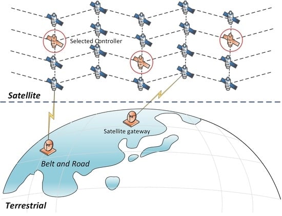
The software-defined STIN architecture is depicted in Figure 2. It consists of three planes: the management plane, data plane, and control plane. The entities in the management plane are deployed on the terrestrial network to realize mobility and handover management functions. The ground contains infrastructure such as base stations, gateways, vehicles, ships, computers, as well as mobile phones. The terrestrial network communicates with the satellite network via satellite gateways in the management plane. The LEO satellites are responsible for carrying the switch function and forwarding data packets in the data plane. It is assumed that each satellite can host the control unit. Several LEO satellites are selected as controllers to achieve the distributed control of the STIN, and they are only responsible for communicating with the other LEO satellites under their coverage instead of all LEO satellites in the space network.
The network topology of the STIN in each time slot is defined as a graph , where V represents the set of the network nodes (LEO satellites and satellite gateways), and E represents the set of links, i.e., ISLs and user data links (UDLs). Let denote the set of satellite nodes, denote the set of satellite gateways, and denote the set of satellite controllers.
For the communication between the satellites selected as SDN controllers and the potential controller set, SDN switches collect the status instruction via the existing ISLs. Almost every satellite has four ISLs [36]: two intra-plane ISLs which link to the adjacent satellites in the same orbit plane and two inter-plane ISLs which link to the satellites in the left- or right-neighbor orbit plane. However, the satellites which rotate in opposite directions in two adjacent orbit planes only have three ISLs: two intra-plane ISLs and one inter-plane ISL. The length of the intra-plane ISLs is constant, which is computed as:
where is the radius of the orbit, and M is the number of satellites in an orbit.
The length of the inter-plane ISLs is constantly varying due to the movements of the satellites, which is computed as:
where refers to the latitude, and N is the number of orbits. The length of inter-plane ISLs decreases as the latitude increases. Once the satellites move into the polar region, the inter-plane ISLs break.
Furthermore, we assume that the speed of transmitting flows is equal to the speed of light. That is to say, the length of ISLs also determines the latency in the STIN. Although controllers are the same as satellite switches physically, they are separated from each other in function. The position of controllers determines the way to process traffic flows, and the corresponding ISLs are regarded as control paths.
3.2. Energy Consumption Model
Due to the dynamic nature of requests from users, we need to establish a traffic model related to the number of people on the Earth. The number of Internet users and the traffic demands can be calculated based on the statistical data [37]. The Earth’s surface is divided into areas for simplification. Figure 3 shows the traffic demands over the world, in which for every Internet users in each area, the traffic demand is 1 Mbps [38]. Moreover, if the number of Internet users is less than in an area, the traffic demands are also set as 1 Mbps.
We assume each satellite is equipped with a switch processing unit. In each time slot, the area is assigned to the nearest satellite for flow processing. The traffic flows of each satellite are the sum of flows in its managed area. The energy consumption of traffic flows in satellites mainly covers three parts: sending, on-board processing, and receiving.
Formally, the energy consumption of sending data by switch is defined as:
where is the sending rate of switch , is the energy consumption of switch at the maximum sending rate, and [39] is the energy consumption weight function.
Similarly, the energy consumption of receiving data by switch is defined as:
where is the receiving rate of switch , and is the energy consumption of switch at the maximum receiving rate.
The energy consumption of on-board processing by switch is defined as:
where is the size of the flow setup request message, is the size of the flow table entry, is the energy consumption of matching, and is the energy consumption of executing.
If switch is sending flows to switch , the corresponding energy consumption is defined as:
In this way, the energy consumption of the flow setup request between switch s and controller c is defined as:
where equals 1, indicating that the ISL belongs to the control path, and it equals 0, indicating the ISL does not belong to it.
Moreover, the energy consumption among controllers for synchronizing controller information is defined as:
where equals 1, indicating that there exists the shortest path ISL connecting controllers, and it equals 0 indicating the ISL does not belong to the shortest path.
We formulate the EECP problem under the latency constraint in the software-defined STIN, which is expressed as the following optimization problem:
where is the energy consumption between satellite gateway g and satellite s; equals 1 if the satellite s is assigned to controller c and equals 0 otherwise; equals 1 if the satellite gateway g is assigned to satellite s and equals 0 otherwise.
Constraint (10) ensures that each satellite s is controlled by exactly one controller c. Constraint (11) guarantees that the switch is connected to a node where a controller resides; equals 1 if the satellite node c is selected as the controller and equals 0 otherwise. Constraint (12) means that the control paths need to meet the latency constraint ; represents the propagation latency of the path from satellite s to controller c. Constraint (13) ensures that controller c controls at most number of switches; ; is the number of satellites; and is the number of controllers.
4. Heuristic Placement Algorithm
The most intuitive way to solve the EECP problem is to enumerate all the possible controller placement schemes and select the best among them as the final result. However, due to its high time complexity, this method is not suitable for such large-scale STINs. In this paper, we focus on a heuristic-based algorithm to solve the EECP problem proposed in Section 3.2. The SA [40] is regarded as a heuristic approach based on Monte Carlo, which searches for the global optimal solution for the decrease in temperature. The proposed modified simulated annealing placement (MSAP) algorithm introduces the greedy method into the SA algorithm to obtain the optimal controller placement with minimum energy consumption.
The greedy initial (GI) algorithm is used to obtain the initial set of controller placements for the MSAP algorithm. The details of the GI algorithm are shown in Algorithm 1. The input consists of the network topology graph and preset controllers k deployed on STIN. We initialize the set of controllers (line 1) and then calculate the minimum energy consumption by Equation (9) between any two nodes (line 2). The energy consumption is stored in the matrix. The initial placement solution is obtained by iterating k times (line 3). In each iteration of the for-loop, we choose a new potential node as a controller from the candidate controllers and add it to the list of controllers (line 5). We need to calculate the energy consumption using Equation (9) under the current controller deployment (line 6) and record the minimum value (line 8). Once all the candidate nodes have been traversed (line 9), we find the placement scheme with the minimum energy consumption (line 10). The set of controllers can be available initially (line 12).
| Algorithm 1 Greedy Initial Algorithm (GI). |
|
The details of the MSAP algorithm are described in Algorithm 2, in which the input is the same as Algorithm 1. We first initialize the parameters, including the initial temperature , the final temperature , and the annealing coefficient (line 1). The output of Algorithm 1 is the initial state of the set of controllers (line 2), and the energy consumption is calculated (line 3). In each while-loop, the temperature decreases until the system reaches a balance point (line 4). We find the placement solution with the minimum energy consumption in all the new neighbor solutions at this stage (line 5). The set of controllers and energy consumption will be updated if the new solution achieves lower energy consumption (line 6 to line 9). In order to avoid falling into the local optimal, the probability of the current worse solution is accepted, where and belong to (line 10 to line 14). When the temperature decreases until the solid reaches its stable state, the while-loop ends (line 16). In this way, we obtain the set of controllers and energy consumption (line 18).
The computational complexity of the MSAP algorithm is discussed as follows. The time complexity of the minimum energy consumption between any two nodes is . Thus, the running time of the initial set of controllers is . So, the computational time complexity of MSAP is , where t is the iteration number.
| Algorithm 2 Modified Simulated Annealing Placement Algorithm (MSAP). |
|
5. Simulation Results
In order to demonstrate the performance of the proposed MSAP algorithm, in this section, we first introduce the simulation setup, then give an analysis of the proposed architecture which deploys controllers on LEO satellites based on the MSAP algorithm. Finally, we compare the MSAP algorithm with other algorithms.
5.1. Simulation Setup
In the simulation, we construct an STIN simulation scenario based on the real-world parameters from the STK (Systems Tool Kit) [41], which models the LEO constellation and satellite gateways. We use the Iridium constellation and place five satellite gateways in the countries of the Belt and Road. The distribution of satellite gateways is listed in Table 2. The Iridium constellation consists of 66 satellites. They are evenly distributed in six orbit planes with a height of 780 km and an orbital inclination of 86.4°. Considering the dynamic changes in the satellite network, we captured the network topology on 1 January 2020 12 PM GMT for simulation, which is shown in Figure 4.
Furthermore, MATLAB is used to implement the MSAP algorithm, and the energy consumption and average latency are used as evaluation indices. The values of key simulation parameters are listed in Table 3 [39,42]. The port rate of the switch R is set to different values according to the traffic demands.
5.2. Analysis of the Architecture
The location of controllers determines the control mode of network, which also effects the efficiency of message processing. The controllers deployed on the ground network are often located at the pre-selected geographical location [43]. We compare the performance of the controller located on the LEO satellites with the satellite gateways on the ground.
Figure 5 shows the effect of controller location on energy consumption and average latency. We compare the architecture deployed controllers on LEO satellite with controllers on satellite gateway. Since there are five satellite gateways deployed on the Belt and Road, the number of controllers is set from one to five for comparison. When the number of controllers is equivalent, the architecture which deploys controllers on LEO satellites consumes less energy and achieves lower latency than the controllers on the satellite gateway. In addition, when there are five controllers on LEO satellites, it saves nearly 30% on energy consumption and latency compared to controllers on the satellite gateway.
The controllers on the satellite gateway are located on the Belt and Road and are close to each other in geography. The satellite gateway is prone to reaching its capacity with the increased number of controllers. The proposed software-defined STIN architecture considers the controllers on LEO satellites. We also adopt the MSAP algorithm to enumerate the optimal location of controllers. In this manner, it reduces energy consumption and average latency with the increased number of controllers.
5.3. Comparison with Different Algorithms
In order to evaluate the performance of the MSAP algorithm, we adopt the Random, K-means [44], Greedy [19], and SAP [45] algorithms as benchmarks:
- Random algorithm means randomly choosing nodes as controllers. To eliminate the effect of randomness, we run the algorithm 10 times and take the average result as the final output.
- K-means [44] belongs to the clustering algorithm. By calculating the energy consumption between nodes and the selected controllers, the nodes are divided into multiple clusters in STIN.
- Greedy algorithm [19] provides locally optimal results that approximate globally optimal solutions. The controllers are selected one by one, and it assures that the energy consumption of STIN achieves the optimal results at this stage.
- SA algorithm [45] approximates the global optimum solution through a random search technique. The nodes are selected as controllers once the energy consumption of STIN reaches a thermal equilibrium point.
We measure the performance of these algorithms from the following aspects.
(1) Energy Consumption: Energy consumption can be calculated by the definition in Equation (9). Figure 6 shows the energy consumption with the different number of controllers in STIN. The number of controllers is assigned from one to seven. It can be noted that energy consumption calculated by the five algorithms decreases first and then increases as there are more controllers in the STIN. This is due to the increased number of controllers, which places an unsupportable burden on the network. Consequently, we need to strike a balance between the control mechanism and economic concerns.
Moreover, the proposed MSAP outperforms other algorithms in energy consumption. MSAP adopts the advantages of Greedy and SA, which finds the initial optimal results by the Greedy algorithm and then achieves the global optimal solutions by the SA algorithm. Especially when the number of controllers is set as 1, MSAP has the same results as the Greedy algorithm. In addition, the initial step of controller placement for SA and K-means impacts the final results. We run the Random, K-means, and SA algorithms multiple times, and their results fluctuate within a range. Due to the stochastic property, the Random algorithm can hardly achieve approximate results and shows the largest fluctuation in energy consumption of all the tested algorithms. Overall, the performance of the MSAP algorithm is better than other algorithms in energy consumption.
To further evaluate the performance of the five algorithms, we compare the energy consumption for controllers. That means we only consider the energy consumption for synchronizing control information. The results of energy consumption are shown in Figure 7. It is worth noting that the more controllers in STIN, the more energy will be consumed for synchronizing information. The energy consumption for controllers is similar in different algorithms. The proposed MSAP algorithm consumes the least energy out of the algorithms tested when the number of controllers is set as seven. That mainly results from the consideration of the global and local optimal strategies for the locations of controllers. Moreover, affected by the number of controllers, the energy consumption calculated by the SAP algorithm and K-means algorithm fluctuates greatly.
(2) Latency with Minimum Energy Consumption: We also consider the network latency of the controller placement solution with the minimum energy consumption. It is defined as the ratio of distance and propagation speed. The distance represents the sum of distance in the shortest path between controllers and other nodes (switches and gateways), and the propagation speed is regarded as the speed of light ( km/s).
Figure 8 shows the average latency with different numbers of controllers in STIN. It can be found that the average latency decreased first, then increased with the number of controllers. The tendency of Figure 8 is similar to Figure 6. When the number of controllers exceeds the optimal range, it brings a further increased burden on the network. Specifically, the average latencies calculated by the Greedy, SA, and MSAP algorithms are identical when there is only one controller. The proposed MSAP algorithm achieves a lower average latency than the other algorithms when multiple controllers are deployed on the STIN. Random and K-means algorithms still do not achieving optimal performance in average latency, and they are unsuitable for solving the proposed EECP problem.
We also focus on the average latency between controllers, which represents the average latency for each controller link in the LEO satellite network. It reflects the distribution of controllers in the LEO satellite network. The average latency of different number of controllers is shown in Figure 9. The latency calculated by MSAP, SAP, and Greedy algorithms decreased by nearly 35 ms, 45 ms, and 30 ms, respectively. However, Random and K-means present the tendency to be stochastic, they are not highly related to the number of controllers, and the distribution of controllers is not ruleable.
(3) Benefit-to-Cost Ratio (BCR): BCR refers to a proportional reduction with respect to one controller. It is defined as , where represents the energy consumption when k controllers are deployed on the LEO satellite network. The higher the value of the BCR, the better the result.
Table 4 shows the BCR of energy consumption. When the number of controllers increases, the BCR obtained by the five algorithms shows a decreasing tendency. It needs at least four controllers to reduce the energy consumption to half in the three algorithms. BCR follows the law of diminishing returns. When the number of controllers reaches the capability in the STIN, it will obtain minor benefits in return. The trade-off between cost and energy consumption should be considered while selecting the number of controllers.
6. Conclusions
The rapid development of the economy derives more and more applications which are transmitted by satellites. However, a large amount of energy is required to maintain the flow of satellite traffic. Aiming to save energy consumption in a software-defined STIN, in this paper, we researched the EECP problem in the countries along the Belt and Road. The energy consumption model was developed to describe the energy consumption of ISL (switch-to-controller) and UDL (gateway-to-satellite). Based on the model, we considered traffic demands in the different geographical locations, which were then formulated as an optimization problem. To solve the EECP problem, we proposed the MSAP algorithm to compute the optimal locations of controllers. The simulation was evaluated by real-world parameters with an LEO constellation and Internet usage traces. The results indicated that the considered SDN-enabled architecture achieved superior performance to the controllers deployed on the satellite gateway. In the performance evaluation, the satellite controller placement provided by the MSAP algorithm outperformed other algorithms in network energy consumption and latency.
Author Contributions
Conceptualization, L.W. and C.C.; methodology, L.W. and C.C.; software, C.C.; validation, L.W. and C.C; formal analysis, L.W. and C.C.; investigation, L.W. and C.C; resources, L.W., C.C. and Y.L.; data curation, C.C.; writing—original draft preparation, C.C.; writing—review and editing, L.W., C.C. and Y.L.; visualization, L.W.; supervision, Y.L. and Y.W.; project administration, Y.L. and Y.W.; funding acquisition, Y.L. All authors have read and agreed to the published version of the manuscript.
Funding
This work was supported by the National Key Research and Development Program of China (No.2019YFB1803103) and in part by the BUPT Excellent Ph.D. Students Foundation (No.CX2021113).
Institutional Review Board Statement
Not applicable.
Informed Consent Statement
Not applicable.
Data Availability Statement
The data presented in this study are available on request from the corresponding author.
Acknowledgments
The authors would like to thank the anonymous reviewers for their valuable comments and helpful suggestions.
Conflicts of Interest
The authors declare no conflict of interest.
Abbreviations
The following abbreviations are used in this manuscript:
| STIN | Satellite Terrestrial Integrated Network |
| SDN | Software-Defined Networking |
| GEO | Geostationary Earth Orbit |
| MEO | Medium Earth Orbit |
| LEO | Low Earth Orbit |
| HAP | High-Altitude Platforms |
| LAP | Low-Altitude Platforms |
| ISL | Inter-Satellite Links |
| UDL | User Data Links |
| VR | Virtual Reality |
| IoT | Internet of Things |
| CPP | Controller Placement Problem |
| EECP | Energy-Efficient Controller Placement |
| SA | Simulated Annealing |
| SAP | Simulated Annealing Placement |
| MSAP | Modified Simulated Annealing Placement |
| GI | Greedy Initial |
| 6G | 6th Generation Mobile Networks |
| STK | Systems Tool Kit |
| QoS | Quality of Service |
| WAN | Wide-Area Network |
| GA | Genetic Algorithm |
| PSO | Particle Swarm Optimization |
| AA | Approximation Algorithm |
References
- Bacco, M.; Davoli, F.; Giambene, G.; Gotta, A.; Luglio, M.; Marchese, M.; Patrone, F.; Roseti, C. Networking Challenges for Non-Terrestrial Networks Exploitation in 5G. In Proceedings of the 2019 IEEE 2nd 5G World Forum (5GWF), Dresden, Germany, 30 September–2 October 2019; pp. 623–628. [Google Scholar]
- Saad, W.; Bennis, M.; Chen, M. A Vision of 6G Wireless Systems: Applications, Trends, Technologies, and Open Research Problems. IEEE Netw. 2020, 34, 134–142. [Google Scholar] [CrossRef] [Green Version]
- Foust, J. SpaceX’s Space-Internet Woes: Despite Technical Glitches, the Company Plans to Launch the First of Nearly 12,000 Satellites in 2019. IEEE Spectr. 2019, 56, 50–51. [Google Scholar] [CrossRef]
- Radtke, J.; Kebschull, C.; Stoll, E. Interactions of the Space Debris Environment with Mega Constellations—Using the Example of the OneWeb Constellation. Acta Astronaut. 2017, 131, 55–68. [Google Scholar] [CrossRef]
- Liu, J.; Shi, Y.; Fadlullah, Z.M.; Kato, N. Space-Air-Ground Integrated Network: A Survey. IEEE Commun. Surv. Tutor. 2018, 20, 2714–2741. [Google Scholar] [CrossRef]
- Yao, H.; Wang, L.; Wang, X.; Lu, Z.; Liu, Y. The Space-Terrestrial Integrated Network: An Overview. IEEE Commun. Mag. 2018, 56, 178–185. [Google Scholar] [CrossRef]
- Kreutz, D.; Ramos, F.M.V.; Veríssimo, P.E.; Rothenberg, C.E.; Azodolmolky, S.; Uhlig, S. Software-Defined Networking: A Comprehensive Survey. Proc. IEEE 2015, 103, 14–76. [Google Scholar] [CrossRef] [Green Version]
- Yuan, S.; Peng, M.; Sun, Y.; Liu, X. Software Defined Intelligent Satellite-Terrestrial Integrated Networks: Insights and Challenges. Digit. Commun. Netw. 2022. [Google Scholar] [CrossRef]
- Heller, B.; Sherwood, R.; McKeown, N. The Controller Placement Problem. SIGCOMM Comput. Commun. Rev. 2012, 42, 473–478. [Google Scholar] [CrossRef] [Green Version]
- Andrae, A.S.G.; Edler, T. On Global Electricity Usage of Communication Technology: Trends to 2030. Challenges 2015, 6, 117–157. [Google Scholar] [CrossRef] [Green Version]
- Liu, H.; Fang, C.; Miao, Y.; Ma, H.; Zhang, Q.; Zhou, Q. Spatio-Temporal Evolution of Population and Urbanization in the Countries along the Belt and Road 1950–2050. J. Geogr. Sci. 2018, 28, 919–936. [Google Scholar] [CrossRef]
- Isong, B.; Molose, R.R.S.; Abu-Mahfouz, A.M.; Dladlu, N. Comprehensive Review of SDN Controller Placement Strategies. IEEE Access 2020, 8, 170070–170092. [Google Scholar] [CrossRef]
- Lu, J.; Zhang, Z.; Hu, T.; Yi, P.; Lan, J. A Survey of Controller Placement Problem in Software-Defined Networking. IEEE Access 2019, 7, 24290–24307. [Google Scholar] [CrossRef]
- Wang, T.; Liu, F.; Xu, H. An Efficient Online Algorithm for Dynamic SDN Controller Assignment in Data Center Networks. IEEEACM Trans. Netw. 2017, 25, 2788–2801. [Google Scholar] [CrossRef]
- Bera, S.; Misra, S.; Saha, N. Traffic-Aware Dynamic Controller Assignment in SDN. IEEE Trans. Commun. 2020, 68, 4375–4382. [Google Scholar] [CrossRef]
- Singh, A.K.; Maurya, S.; Kumar, N.; Srivastava, S. Heuristic Approaches for the Reliable SDN Controller Placement Problem. Trans. Emerg. Telecommun. Technol. 2020, 31, e3761. [Google Scholar] [CrossRef]
- Liao, C.; Chen, J.; Guo, K.; Liu, S.; Chen, J.; Gao, D. MODECP: A Multi-Objective Based Approach for Solving Distributed Controller Placement Problem in Software Defined Network. Sensors 2022, 22, 5475. [Google Scholar] [CrossRef]
- Liu, J.; Liu, J.; Xie, R. Reliability-based controller placement algorithm in software defined networking. Comput. Sci. Inf. Syst. 2016, 13, 547–560. [Google Scholar] [CrossRef]
- Salam, R.; Bhattacharya, A. Efficient Greedy Heuristic Approach for Fault-Tolerant Distributed Controller Placement in Scalable SDN Architecture. Clust. Comput. 2022, 25, 4543–4572. [Google Scholar] [CrossRef]
- Aravind, P.; Varma, G.P.S.; Reddy, P.V.G.D.P. Simulated Annealing Based Optimal Controller Placement in Software Defined Networks with Capacity Constraint and Failure Awareness. J. King Saud. Univ. Comput. Inf. Sci. 2022, 34, 5721–5733. [Google Scholar] [CrossRef]
- Maity, I.; Dhiman, R.; Misra, S. EnPlace: Energy-Aware Network Partitioning for Controller Placement in SDN. IEEE Trans. Green Commun. Netw. 2022. [Google Scholar] [CrossRef]
- Ruiz-Rivera, A.; Chin, K.-W.; Soh, S. GreCo: An Energy Aware Controller Association Algorithm for Software Defined Networks. IEEE Commun. Lett. 2015, 19, 541–544. [Google Scholar] [CrossRef]
- Hu, Y.; Luo, T.; Beaulieu, N.C.; Deng, C. The Energy-Aware Controller Placement Problem in Software Defined Networks. IEEE Commun. Lett. 2017, 21, 741–744. [Google Scholar] [CrossRef]
- Fernandez-Fernandez, A.; Cervello-Pastor, C.; Ochoa-Aday, L. Achieving Energy Efficiency: An Energy-Aware Approach in SDN. In Proceedings of the 2016 IEEE Global Communications Conference (GLOBECOM), Washington, DC, USA, 4–8 December 2016; pp. 1–7. [Google Scholar]
- Liu, J.; Shi, Y.; Zhao, L.; Cao, Y.; Sun, W.; Kato, N. Joint Placement of Controllers and Gateways in SDN-Enabled 5G-Satellite Integrated Network. IEEE J. Sel. Areas Commun. 2018, 36, 221–232. [Google Scholar] [CrossRef]
- Bi, Y.; Han, G.; Xu, S.; Wang, X.; Lin, C.; Yu, Z.; Sun, P. Software Defined Space-Terrestrial Integrated Networks: Architecture, Challenges, and Solutions. IEEE Netw. 2019, 33, 22–28. [Google Scholar] [CrossRef]
- Shen, Y.; Chen, W.; Liu, J. Joint Placement of Gateways and Controllers in SDN-Enabled Space-Ground Integration Network. In Proceedings of the 2022 Asia Conference on Electrical, Power and Computer Engineering (EPCE 2022), Shanghai, China, 22 April 2022; ACM: New York, NY, USA, 2022; pp. 1–6. [Google Scholar]
- Bao, J.; Zhao, B.; Yu, W.; Feng, Z.; Wu, C.; Gong, Z. OpenSAN: A Software-Defined Satellite Network Architecture. In Proceedings of the 2014 ACM conference on SIGCOMM, Chicago, IL, USA, 17 August 2014; ACM: New York, NY, USA, 2014; pp. 347–348. [Google Scholar]
- Zhang, Z.; Zhao, B.; Yu, W.; Wu, C. Poster: An Efficient Control Framework for Supporting the Future SDN/NFV-Enabled Satellite Network. In Proceedings of the 23rd Annual International Conference on Mobile Computing and Networking, Snowbird, UT, USA, 16–20 October 2017; Association for Computing Machinery: New York, NY, USA, 2017; pp. 603–605. [Google Scholar]
- Papa, A.; De Cola, T.; Vizarreta, P.; He, M.; Mas Machuca, C.; Kellerer, W. Dynamic SDN Controller Placement in a LEO Constellation Satellite Network. In Proceedings of the 2018 IEEE Global Communications Conference (GLOBECOM), Abu Dhabi, United Arab Emirates, 9–13 December 2018; pp. 206–212. [Google Scholar]
- Chen, C.; Liao, Z.; Ju, Y.; He, C.; Yu, K.; Wan, S. Hierarchical Domain-Based Multi-Controller Deployment Strategy in SDN-Enabled Space-Air-Ground Integrated Network. IEEE Trans. Aerosp. Electron. Syst. 2022. [Google Scholar] [CrossRef]
- Han, Z.; Xu, C.; Xiong, Z.; Zhao, G.; Yu, S. On-Demand Dynamic Controller Placement in Software Defined Satellite-Terrestrial Networking. IEEE Trans. Netw. Serv. Manag. 2021, 18, 2915–2928. [Google Scholar] [CrossRef]
- Wu, S.; Chen, X.; Yang, L.; Fan, C.; Zhao, Y. Dynamic and Static Controller Placement in Software-Defined Satellite Networking. Acta Astronaut. 2018, 152, 49–58. [Google Scholar] [CrossRef]
- Liao, Z.; Chen, C.; Ju, Y.; He, C.; Jiang, J.; Pei, Q. Multi-Controller Deployment in SDN-Enabled 6G Space–Air–Ground Integrated Network. Remote Sens. 2022, 14, 1076. [Google Scholar] [CrossRef]
- Qu, H.; Xu, X.; Zhao, J.; Yue, P. An SDN-Based Space-Air-Ground Integrated Network Architecture and Controller Deployment Strategy. In Proceedings of the 2020 IEEE 3rd International Conference on Computer and Communication Engineering Technology (CCET), Beijing, China, 14–16 August 2020; pp. 138–142. [Google Scholar]
- Radhakrishnan, R.; Edmonson, W.W.; Afghah, F.; Rodriguez-Osorio, R.M.; Pinto, F.; Burleigh, S.C. Survey of Inter-Satellite Communication for Small Satellite Systems: Physical Layer to Network Layer View. IEEE Commun. Surv. Tutor. 2016, 18, 2442–2473. [Google Scholar] [CrossRef] [Green Version]
- Internet Usage Statistics. [Online]. 2015. Available online: http://www.internetworldstats.com/stats.htm (accessed on 31 July 2022).
- Yang, Y.; Xu, M.; Wang, D.; Wang, Y. Towards Energy-Efficient Routing in Satellite Networks. IEEE J. Sel. Areas Commun. 2016, 34, 3869–3886. [Google Scholar] [CrossRef]
- Lombardo, A.; Panarello, C.; Reforgiato, D.; Schembra, G. Measuring and Modeling Energy Consumption to Design a Green NetFPGA Giga-Router. In Proceedings of the 2012 IEEE Global Communications Conference (GLOBECOM), Anaheim, CA, USA, 3–7 December 2012; pp. 3062–3067. [Google Scholar]
- Saha, B.K.; Misra, S.; Pal, S. SeeR: Simulated Annealing-Based Routing in Opportunistic Mobile Networks. IEEE Trans. Mob. Comput. 2017, 16, 2876–2888. [Google Scholar] [CrossRef]
- AGI. Systems Tool Kit (STK). Available online: https://www.agi.com/products/engineering-tools (accessed on 15 December 2021).
- Yao, G.; Bi, J.; Li, Y.; Guo, L. On the Capacitated Controller Placement Problem in Software Defined Networks. IEEE Commun. Lett. 2014, 18, 1339–1342. [Google Scholar] [CrossRef]
- del Portillo, I.; Cameron, B.; Crawley, E. Ground Segment Architectures for Large LEO Constellations with Feeder Links in EHF-Bands. In Proceedings of the 2018 IEEE Aerospace Conference, Big Sky, MT, USA, 3–10 March 2018; pp. 1–14. [Google Scholar]
- Wang, G.; Zhao, Y.; Huang, J.; Duan, Q.; Li, J. A K-Means-Based Network Partition Algorithm for Controller Placement in Software Defined Network. In Proceedings of the 2016 IEEE International Conference on Communications (ICC), Kuala Lumpur, Malaysia, 23–27 May 2016; IEEE: Piscataway, NJ, USA, 2016; pp. 1–6. [Google Scholar]
- Chang, C.; Liu, Y.; Wang, Y. Failure-Based Multi-Controller Placement in Software Defined Satellite Networking. In Proceedings of the 2021 IEEE International Conference on Communications Workshops (ICC Workshops), Montreal, QC, Canada, 14–23 June 2021; pp. 1–6. [Google Scholar]
Figure 1.
The typical architecture of the STIN.

Figure 2.
The overview of the software-defined STIN architecture.

Figure 3.
The number of Internet users, divided by [38].
Figure 3.
The number of Internet users, divided by [38].

Figure 4.
The snapshot of Iridium network at 1 January 2020 12 PM GMT (the satellite nodes are shown with blue circles, and the satellite gateways are denoted with orange).
Figure 4.
The snapshot of Iridium network at 1 January 2020 12 PM GMT (the satellite nodes are shown with blue circles, and the satellite gateways are denoted with orange).

Figure 5.
Energy consumption and average latency when controllers on different locations.

Figure 6.
Energy consumption with the different number of controllers in STIN.

Figure 7.
Energy consumption for controllers in the LEO satellite network.

Figure 8.
Latency with the different number of controllers in STIN.

Figure 9.
Latency for each control link in the LEO satellite network.


Table 1.
Comparison of the proposed scheme with state-of-the-art methods.
| Ref. | Locations | Algorithms | Metrics | |||
|---|---|---|---|---|---|---|
| Latency | Cost | Reliability | Load | |||
| [35] | Air | K-means | ✓ | |||
| [25] | Ground | SA | ✓ | ✓ | ||
| [30] | Satellites | ILP | ✓ | |||
| [31] | Ground, Satellites | GA | ✓ | ✓ | ||
| [32] | Satellites | AA | ✓ | |||
| [33] | Satellites | PSO | ✓ | ✓ | ✓ | |
| [34] | Satellites | SA | ✓ | |||
| Proposed | Satellites | SA | ✓ | ✓ | ✓ | ✓ |
Table 2.
Distribution of satellite gateways.
| Satellite Gateway | Country, City | Longitude | Latitude |
|---|---|---|---|
| SG1 | China, Beijing | 116.4 | 39.9 |
| SG2 | Indonesia, Jakarta | 106.8 | −6.3 |
| SG3 | Russia, Moskva | 37.7 | 55.8 |
| SG4 | Kazakhstan, Almaty | 76.9 | 43.3 |
| SG5 | Saudi Arabia, Al Madinah | 39.7 | 24.4 |
Table 3.
Simulation parameters.
| Parameter | Value |
|---|---|
| (mJ) | 7.639 |
| (mJ) | 1.944 |
| (Byte) | 160 |
| (nJ/B) | 5.634 |
| (nJ/B) | 8.406 |
| R (Mbps) | |
| (Byte) | 280 |
| (C) | 1 |
| (C) | 0.0001 |
| 0.75 |
Table 4.
Benefit-to-Cost Ratio of Energy Consumption.
| Methods | Number of Controllers | ||||||
|---|---|---|---|---|---|---|---|
| 1 | 2 | 3 | 4 | 5 | 6 | 7 | |
| Random | 1 | 0.62 | 0.49 | 0.42 | 0.32 | 0.22 | 0.15 |
| K-means | 1 | 0.70 | 0.60 | 0.39 | 0.32 | 0.25 | 0.15 |
| GI | 1 | 0.61 | 0.46 | 0.38 | 0.26 | 0.20 | 0.16 |
| SAP | 1 | 0.64 | 0.48 | 0.37 | 0.28 | 0.23 | 0.18 |
| MSAP | 1 | 0.66 | 0.53 | 0.41 | 0.32 | 0.25 | 0.20 |
Publisher’s Note: MDPI stays neutral with regard to jurisdictional claims in published maps and institutional affiliations. |
© 2022 by the authors. Licensee MDPI, Basel, Switzerland. This article is an open access article distributed under the terms and conditions of the Creative Commons Attribution (CC BY) license (https://creativecommons.org/licenses/by/4.0/).
Share and Cite
MDPI and ACS Style
Wei, L.; Chang, C.; Liu, Y.; Wang, Y. Energy-Efficient Controller Placement in Software-Defined Satellite-Terrestrial Integrated Network. Remote Sens. 2022, 14, 5561. https://0-doi-org.brum.beds.ac.uk/10.3390/rs14215561
AMA Style
Wei L, Chang C, Liu Y, Wang Y. Energy-Efficient Controller Placement in Software-Defined Satellite-Terrestrial Integrated Network. Remote Sensing. 2022; 14(21):5561. https://0-doi-org.brum.beds.ac.uk/10.3390/rs14215561
Chicago/Turabian StyleWei, Linhui, Chen Chang, Yu Liu, and Yumei Wang. 2022. "Energy-Efficient Controller Placement in Software-Defined Satellite-Terrestrial Integrated Network" Remote Sensing 14, no. 21: 5561. https://0-doi-org.brum.beds.ac.uk/10.3390/rs14215561
Note that from the first issue of 2016, this journal uses article numbers instead of page numbers. See further details here.