Integrating Gaussian Mixture Dual-Clustering and DBSCAN for Exploring Heterogeneous Characteristics of Urban Spatial Agglomeration Areas

Abstract

Exploring the heterogeneous characteristics of the urban expansion process is essential for understanding the dynamics of the urban spatial structure. Many studies focused on depicting the spatio-temporal characteristics based on urban expansion patches. However, measuring heterogeneous characteristics of urban expansion from agglomeration areas comprising the expanded urban construction land patches have not been adequately explored. This study presents a novel approach and two improved indices for characterizing the heterogeneity of urban spatial agglomeration areas during urban expansion. Firstly, we proposed a Gaussian mixture model considering multiple constrains and density-based spatial clustering of applications with noise (DBSCAN) integration method to identify and extract the urban agglomeration areas automatically. Secondly, the gradient analysis and the compact index using the inverse “S” function are introduced to explore the spatio-temporal characteristics from a macrocosmic perspective. Finally, the compactness index (NCI) and normalized dispersion index (NDIS) are improved based on agglomeration area data. The microcosmic heterogeneous characteristics are measured by these two improved indices and the positional offset characteristics indices (POCIS). The method was implemented in the urban area of Changsha, Hunan Province, China in 2005, 2010, and 2015. The results show that (1) compared to that in the Changsha City Master Plan (2003–2020), the recognition rate was higher in the agglomeration areas than others. (2) The overall expansion trend in Changsha transitioned toward decentralization, making Changsha a polycentric city. (3) The agglomeration of urban expansion in the east-west direction became compact; that in the north-south direction became looser; most clusters expanded to the west and a new sub-center would appear. The proposed method can effectively characterize their heterogeneity, which can provide valuable references for urban planning and policymaking.

1. Introduction

The rapid global urbanization process has led to an increase of urban residents in the world from 10% in 1900 to a projected rate of more than 80% by 2050 [1,2,3,4,5]. Along with the rapid population growth, the global extent of urbanized areas is expected to reach 1.2 million km${}^2$ by 2050, which is nearly three times that in 2000 [6,7]. This rapid urban expansion is inseparable from regional and global socioeconomic developments [8]. Changes in urban land use and land cover (LULC), especially excessive and disorderly expansion, can significantly impact the biodiversity and ecology through urban heat islands, cropland loss, and landscape fragmentation, which can hinder sustainability [9,10,11,12]. The measurement and depiction of urban expansion are essential for understanding the urban spatial structure, improving the efficiency of land use, and achieving sustainable development goals.

The urban spatial structure undergoes profound and complex changes during the urban expansion process, which reflects the endogenous mechanism of urban expansion [13,14]. Quantifying the characteristics of urban spatial structures is essential for comprehensively understanding urban expansion and promoting the rationalized expansion of cities [15]. Numerous studies have been conducted to reveal the urban spatial structure from macrocosmic and microcosmic perspectives [16,17,18,19,20]. Studies from a microcosmic perspective mainly focused on the identification of single and multi-centered areas of the city, and investigated their differentiation to analyze the change characteristics at the micro level. However, these central areas are only a part of the spatial structure that includes central areas, cluster areas, and development zones in various planning documents in China. Such areas have a common feature, namely, high levels of agglomeration. Therefore, it is important to identify agglomeration areas and characterize their heterogeneity to understand urban changes from a microscopic perspective.

The clustering method is a core technique [21] for the identification of agglomerated urban patches. Typical clustering methods can be classified into four main categories: hierarchy-, division-, grid-, and density-based methods [22,23,24,25]. Many clustering algorithms have been proposed for the exploration of urban structures [26,27]. However, these methods primarily focus on the clustering of spatial attributes and do not consider their proximity. To consider attributes and spatial dual clustering, Sun et al. [28] proposed an extension of density-based spatial clustering of applications with noise (DBSCAN) in the treatment of non-spatial attributes, the two variables of which are difficult to adjust. Li et al. [29] proposed a spatial clustering method based on the distance and stain recursive retrieval approach, but the determination method and the constraint criteria on the attribute domains were not explicitly defined. Zhang et al. [30] described a self-organized spatial clustering method under dual constraints of space and attributes, which can satisfactorily define the constraints on the space and attribute domains with fewer variables. However, the results of this method provide fragmented small or island-like clusters, and there are no corresponding guidelines to rectify outlier clusters. In the above clustering methods, the spatial locations of urban expansion patches were used as input conditions for the spatial constraint-first clustering method. These methods do not consider attribute constraints and cannot express the multi-dimensional geographical features of patches [30,31,32]. Moreover, existing methods cannot accurately extract the extent of agglomeration clusters of urban sprawl patches, ignoring the spatial relationship of patches with the urban structure, thereby only providing regional-level urban expansion characteristics.

Urban expansion is a multi-dimensional geographic phenomenon, and the urban expansion structure can be expressed as the relationship between the arrangement and composition of new urban patches and existing urban land patches. Several metrics have been developed to assess the urban expansion process and pattern at multiple scales. The techniques employed in these metrics include spatial analysis, landscape metrics, and entropy. Most of the existing methods for describing urban expansion patterns often use static data to analyze features of monocentric or polycentric development, the network, and other regional levels of a single phase. However, the dynamics and local structural features of urban expansion have always been ignored in these methods. Additionally, dynamic indices have been proposed based on the relationship between new and existing urban patches. For example, the multi-order adjacency index (MAI) proposed by Liu et al. [33] is derived from the landscape expansion index proposed by Liu et al. [34], and can be used to measure the dynamic pattern of urban expansion. This approach compensates for defects wherein the landscape expansion index cannot be used to compare the distance between the expansion patches and original patches. Musa et al. [35] proposed 19 factors of the urban expansion process and Karimi et al. [36] used the information entropy model to rank the weights of these factors. These methods mainly focus on measuring the degree of expansion of new urban patches based on the features of neighboring urban land patches and ignore their relationship with urban expansion forms.

The aim of extracting clusters is to describe the urban spatial structure and form at the micro-level. A common description method involves the use of dynamic landscape indices. For urban clusters, two types of dynamic landscape features (the compactness feature and the cluster center of gravity offset feature) are often used to describe the urban structure from a microscopic perspective. Compactness features typically measure the spatial continuity of urban elements using fractal dimensions [37], separation indices [38], percentages of similar neighbors [39], continuity indices [40], and other shape-based landscape patterns. These indices usually rely on geometric relationships, such as the area, perimeter, and radius, to express the quantitative relationships of cities at the microscopic level; however, the description of the spatial form of urban expansion is still unclear. The normalized compactness [41] and normalized dispersion [42] indices are effective in portraying the spatial compactness of cities. The cluster direction offset and group location offset characteristics were proposed to describe the cluster center of gravity offset. However, these two methods are based on image elements, and cannot be applied to other data.

Overall, the existing researches can effectively investigate the overall characteristics of urban expansion between neighboring urban land patches during urban expansion. However, the features of spatio-temporal heterogeneity and agglomeration during urban expansion and local characteristics for expansion form description have not been adequately explored. Hence, this study proposes a novel method for exploring heterogeneous characteristics of urban spatial agglomerations to compensate for the above-mentioned shortcomings. Firstly, in order to address the problem that it is difficult to automatically extract and identify agglomeration areas for urban land expansion patches, a method using the Gaussian mixture dual-clustering model with integrated multi-constraints and DBSCAN algorithm is proposed. Secondly, two improved indices, the NCI and NDIS, are explored, and a common index, the POCIS, is introduced to characterize urban agglomeration areas from different perspectives. Additionally, gradient analysis and the inverse “S” urban land density curve were introduced to depict the overall characteristics of spatio-temporal heterogeneity, which can compensate for the deficiencies in the microscopic perspective [43].

2. Methodology

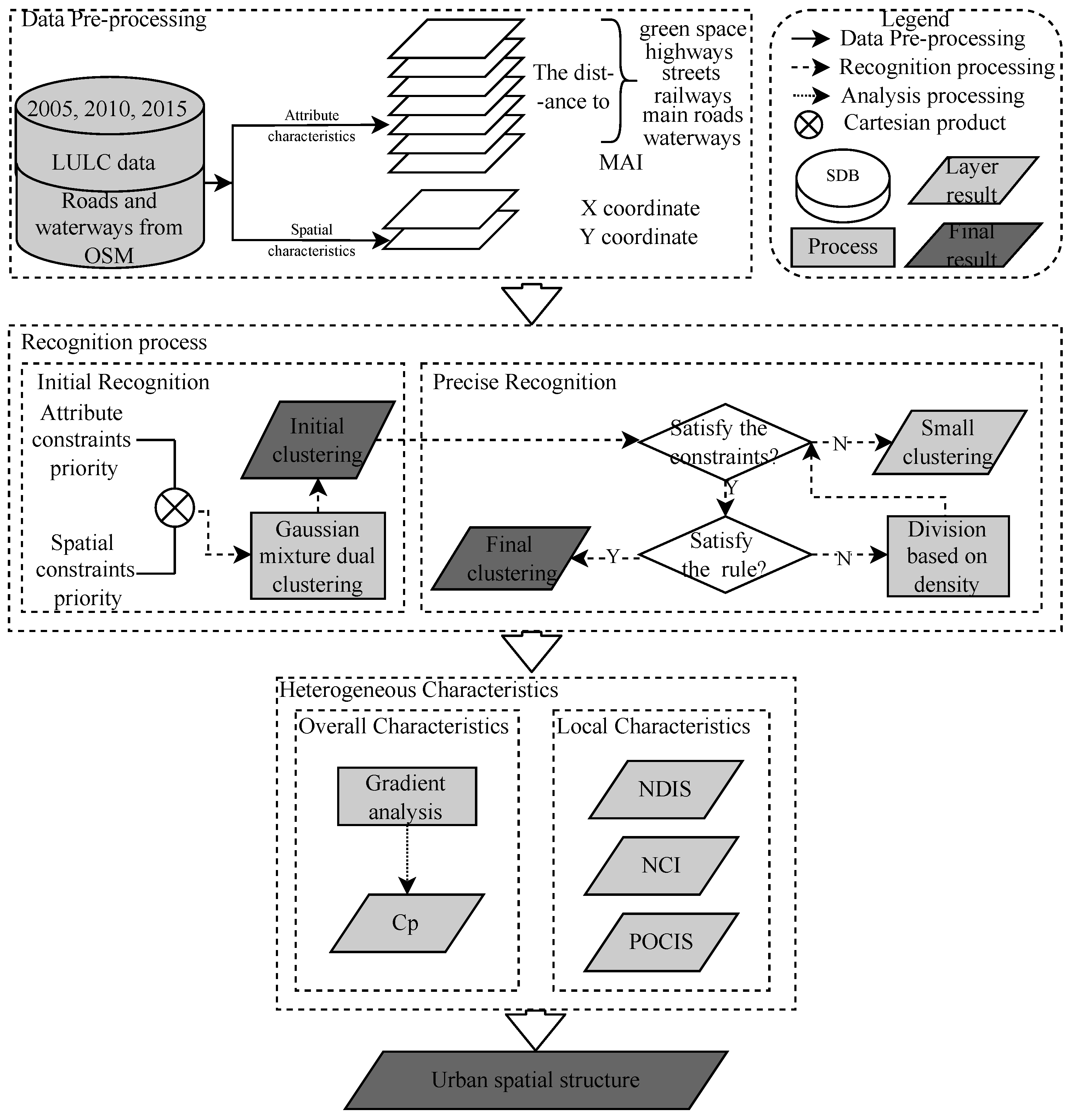
2.1. The Framework for Measuring Agglomeration and Heterogeneous Urban Expansion

As illustrated in Figure 1, the urban agglomeration areas were extracted using the initial and precise recognition from LULC, road, and waterway data after data preprocessing described in Section 3. The initial recognition used the Gaussian mixture dual-clustering model to extract the initial agglomeration information of the city, which is relatively fuzzy and cannot accurately distinguish the boundaries of different clusters. The precise recognition method integrates the multi-constraints and the DBSCAN algorithm to determine the specific cluster boundaries. The key research issues were implemented at two levels using urban agglomeration areas and LULC data. First, we used a gradient analysis method to describe the heterogeneous characteristics of the macrocosmic perspectives. For this purpose, changes in urban compactness were calculated to reflect the changes in heterogeneous characteristics from 2005 to 2015. Second, the heterogeneous characteristics in agglomeration regions were analyzed using the normalized compactness index (NCI), normalized dispersion index (NDIS), and positional offset characteristics indices (POCIS) to reveal the aggregation, dispersion, and offset changes from 2005 to 2015.

2.2. Multi-Order Adjacency Index (MAI)

The design of MAI is based on the degree of adjacency of the spatial relationship between the old and new urban patches [33]. We assume that the buffer distance is M using the multi-order buffer method, which can be adopted to quantify the patch expansion characteristics. Multi-order buffers were established in the new patches until the buffers intersected with the initial patches. The MAI is expressed as follows:

$$MAI=N-\frac{A_i}{A_0}$$

(1)

where N is the number of buffers created for the new patches, $A_0$ is the area of the N-th buffer (outermost buffer), and $A_i$ is the area of the part of the N-th buffer (outermost buffer) that intersects with the old patches.

2.3. Initial Recognition: Gaussian Mixture Dual-Clustering Model

Urban expansion is a complex spatio-temporal process, and the shapes of agglomeration areas vary greatly during this process. The Gaussian mixture model [44] can provide complex density functions by combining multiple Gaussian distributions, increasing the number of Gaussian distributions (mean, covariance matrix, and coefficients of the linear combination), and adjusting the variables of each Gaussian distribution to fit the arbitrary continuous density distributions. Due to the good fitness of GMM for arbitrarily shaped clusters, it is possible to obtain urban agglomeration areas accurately. The model can be represented as follows:

$$p\left(x\right)=\sum _{i=1}^n{\varphi }_{i}p\left(x\right|\mu ,\epsilon )$$

(2)

where the distribution probability is the sum of K Gaussian distributions. Each Gaussian density function becomes a sub-model of the mixture, and each function has its own $\mu$ and $\epsilon$ parameters along with the corresponding weight variables. The weight values must be positive and the sum of all weights must be equal to 1 to ensure that the equation provides a reasonable probability density value.

It is difficult to obtained clusters with both spatial continuity and the spatial distribution pattern of attributes if only spatial feature or similarity in attributes is considered [31]. These spatially continuous clusters with similar attributes can effectively characterize the spatio-temporal homogeneity and heterogeneity in the process of urban expansion. To extract these clusters, the Gaussian mixture dual-clustering combines the results of attribute constraints priority clustering and space constraints priority clustering by a Cartesian product. Since the urban expansion process is particularly complex and the urban patches have different shapes, the use of Gaussian mixture dual model can well extract the cluster classes of various shapes and improve the accuracy of recognition.

The process of Gaussian mixture dual-clustering is described as follows. The set A is $\left\{a_i\right\},i=0,1,\cdots ,l$. each element of A have spatial characteristics (such as latitude and longitude) and attribution characteristics (such as its distance to waterways, wetlands and cropland). Hypothetically, A is aggregated into m classes ($m\le l$) based on the spatial characteristics, denoted as $\left\{S_1,S_2,\cdots ,S_m\right\}$. At the same time, A can be aggregated into n classes ($n\le l$) based on the attributes, denoted as $\left\{P_1,P_2,\cdots ,P_n\right\}$. Then, by employing Cartesian product the dual clustering result of set A is $\left\{[S_1,P_1],[S_2,P_2],\cdots ,[S_j,P_k]\right\}$, which is equal or less than $m\times n$ classes. In order to balance the influences of attribute constraint priority clustering and spatial constraint priority clustering, the category numbers (m and n) of both methods should be the same.

2.4. Precise Recognition

(1)

Constraints Based on the Number or the Area of Patches

After Gaussian mixture dual-clustering, it is inevitable to produce some invalid sparse clusters, which were composed of fragmented polygons due to data processing errors. To explore spatial heterogeneous characteristics of urban expansion, the extracted urban expansion clusters should be as spatially continuous and the attributes of land patch change within each cluster should be homogeneous. Based on these characteristics of clusters and the visual analysis of the initial recognition results, we conclude two types of constraints to remove invalid clusters consisting of fragmented urban expansion patches. Urban expansion patches can be clustered as long as they meet either of these two constraints. The constraints are as follows:

(i)

The number of patches in the cluster should be greater than or equal to n.

(ii)

The total area of the patches in the cluster should be greater than m times the average area of the overall expanded patches.

The number of patches in the cluster should be greater than or equal to n, which is a requirement for the number of clusters. Through statistics and visual analysis of Gaussian mixture dual-clustering results, most of the invalid clusters involve a small number of fragmented urban expansion patches, which may be caused by data process errors. These invalid clusters can cause serious interference to the experimental analysis and need to be removed. However, some valid clusters with a small number of large-scale expansion land patches cannot be extracted while only the number condition of urban expansion patches are used. Therefore, the constraint of land patch areas is explored to allow a small number of large-scale expansion land patches to be aggregated into clusters.

(2)

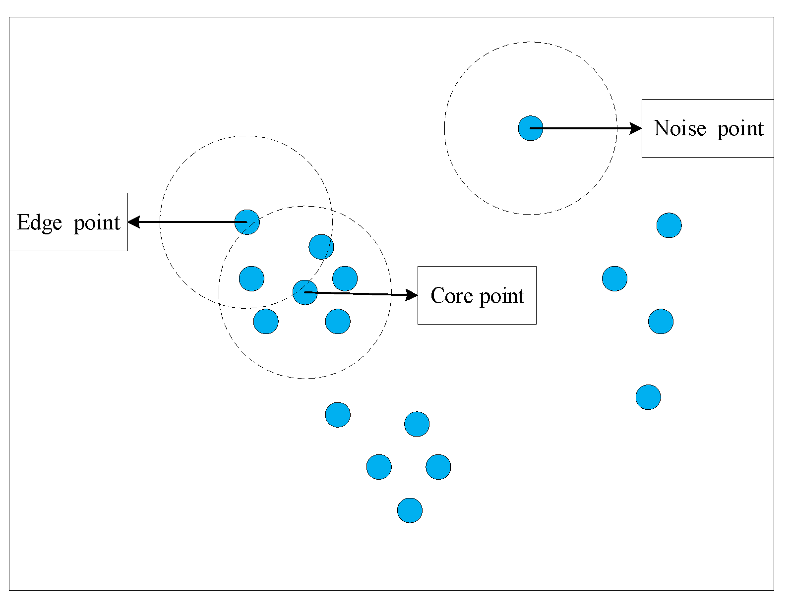
Precise Recognition Based on DBSCAN

After enforcing the constraints based on the number or area of patches, the fragmented, small, and noisy clusters generated by dual clustering were removed. However, some of the remaining clusters were consistent in terms of the attributes but dissimilar in space, and the clusters were highly discrete. In order to reduce the degree of discreteness of clusters, the DBSCAN algorithm [45] was employed. The algorithm was given two variables (neighborhood radius e and minimum neighborhood density threshold $Minpts$) to define three classes of points (Figure 2), which can not only be used to describe the closeness of the sample distribution in the neighborhood of a certain core object, but to also remove some noisy objects.

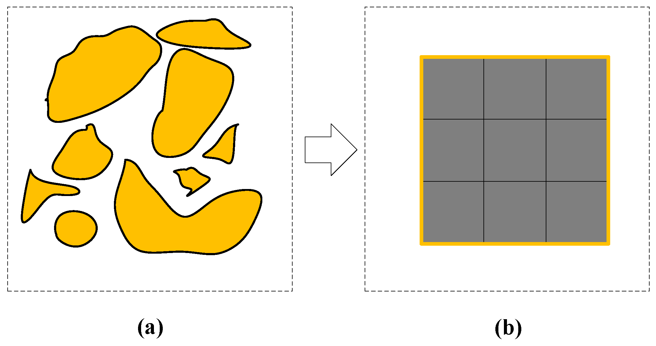
Based on the expansion of the study area, inconsistent regional conditions led to different minimum neighborhood radii. If the number of patches is large, $Minpts$ can choose a smaller value (and vice versa) to consider a large value. The relationship between the minimum number of neighbors and the radius of correlation [46] is expressed as follows:

$$eps=\frac{prod(X_{max}-X_{min})\times Minpts\times \gamma \left(m\right)}{\sqrt{\pi }}$$

(3)

where $X_{max}$ and $X_{min}$ are the maximum and minimum coordinate variables, respectively, along the x-axis. Function $Prod(*)$ is the product of the returned vectors, and $\gamma \left(m\right)$ is the gamma function, whose function body is as follows:

$$\gamma \left(m\right)={\int }_0^{+\infty }{t}^{m-1}{e}^{-t}dt$$

(4)

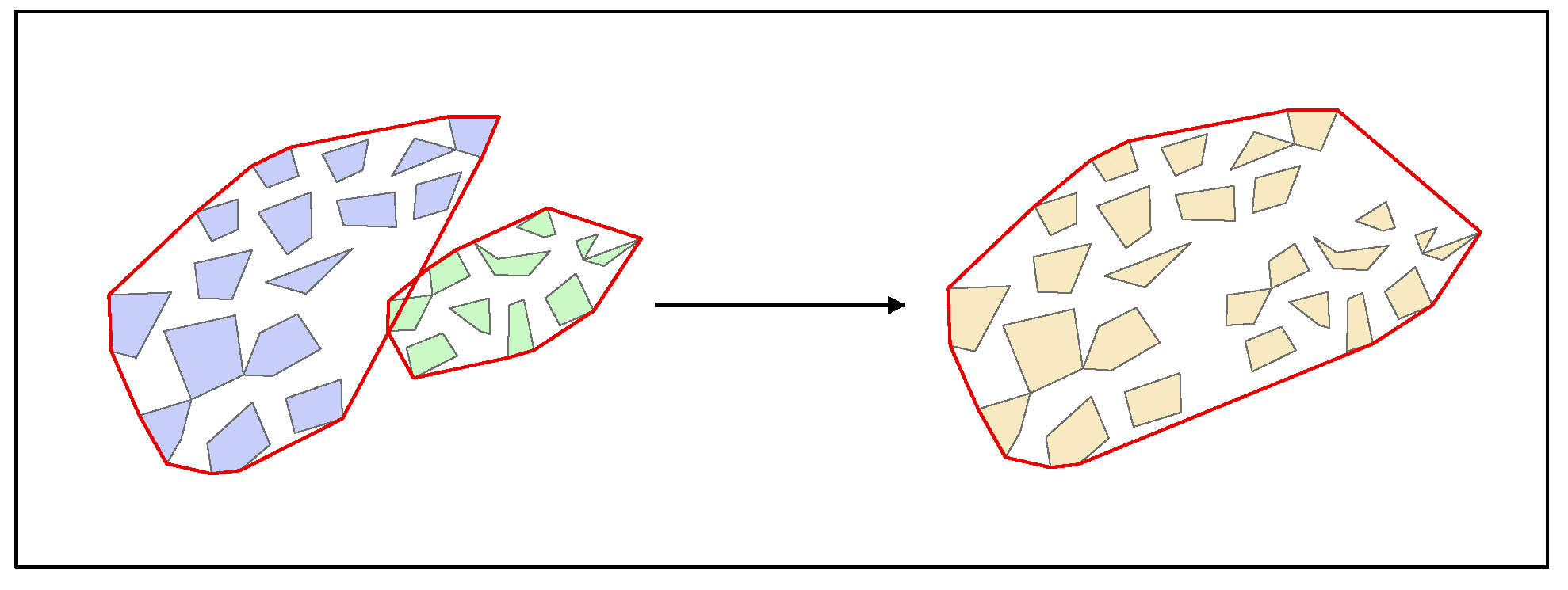
Clustered areas were obtained after conducting DBSCAN clustering. If these clustered areas are not labeled as noise clusters, then satisfy the “Satisfy the rule?” condition in Figure 1. The “Satisfy the rule?” condition is to detect whether the clusters are high-density or not using DBSCAN clustering. Since the number and area of these clusters have changed with respect to their original values, they need to be re-determined with respect to the number or the area constraints of patches. To satisfactorily fit the cluster shape, we used a convex packet to extract the cluster boundary. If a cluster convex packet overlaps with another, these two clusters are then merged into one cluster. The process of merging clusters is shown in Figure 3 and the identification process is shown in Figure 4.

2.5. Heterogeneous Characteristic Analysis

2.5.1. Overall Characteristic Analysis Based on Gradient Analysis and $C_p$ Index

To depict the overall situation, we employed the gradient analysis method in our experiment, which can build a series of equidistant circles through the urban center [47] and can satisfactorily represent the overall changes in the city. Jiao and Dong found that the urban land density showed an inverse “S” pattern on the gradient using the urban land density of each circle through the inverse “S” function to fit the curve [43]. The inverse “S” function compactness index ($C_p$) could be used to depict the macrocosmic compactness of the city, as expressed in the following equations (Equations (5)–(7)).

$$C_p=1-\frac{r_2-r_1}{D}$$

(5)

$$r_1=\frac{D}{2}(\frac{-1.316957}{a}+1)$$

(6)

$$r_2=\frac{D}{2}(\frac{1.316957}{a}+1)$$

(7)

where a, c, and D are the inverse “S” function variables; a is the value determining the slope of the urban value that controls the slope of the density equation curve; c is the land density near the city boundary; and D is the estimated radius of the main urban areas density.

2.5.2. Local Characteristic Indices

(1)

The Normalized Compactness Index (NCI)

The NCI is a mature and valid compactness index based on the gravity model for measuring the compactness of urban sites [41]. The NCI quantifies the urban compactness using the area and distance. In this study, it is applied to the vector patches, which are expressed as follows.

$$CI=\frac{\underset{i=1}{\overset{N-1}{\Sigma }}\underset{j=i+1}{\overset{N}{\Sigma }}\frac{1}{c}\frac{A_i\times A_j}{d_{ij}^2}}{\frac{N(N-1)}{2}}$$

(8)

$$NCI=CI/C{I}_{max}$$

(9)

where $CI$ is the compactness index; i and j are any two patches in a cluster; N is the number of patches; $A_i$ is the area of patch i; $d_{ij}^2$ is the square of the distance between patches i and j; c is a proportionality factor; and $C{I}_{max}$ is the compactness index of the urban sprawl under the standard equal of equal area. The modified equation is changed as follows compared to the original one.

1.

The number of urban patches during the expansion period is less than that of the macrocosmic urban patches; thus, a large enough neighborhood radius is set to include all patches in the cluster within the circle.

2.

According to the characteristics of vector data, five changes were made: (a) each pixel was changed for each expansion patch. (b) The distance was calculated as that between the centers of gravity of each patch. (c) The standard circle was replaced by a standard square. (d) The number of squares was the squared number of patches within the cluster, and the minimum value was four. (e) The side length of the square was expressed as the squared average area of the patches within the cluster.

3.

If the patch area of the cluster was large, resulting in a smaller number of patches (lesser than four), which is inadequate to build a standard square, the patches with larger area can be divided to meet the number of patches required to build a standard square.

The process of generating a square of equal area under the maximum neighborhood range is shown in Figure 5. In general, the calculation results of NCI based on squares are close to those based on circles [41], while it is easier and more convenient to calculate the distance of equal area divided patches from a square than from a circle. Therefore, circles were replaced by squares to calculate the NCI quickly.

(2)

The Normalized Dispersion Index (NDIS)

The NDIS measures the dispersion of a urban land at a local or regional scale by calculating the weighted distance between pixels [42]. In this study, it is used in vector patches. The greater the distance between patches, the greater is the contribution to the DIS value, and the more discrete is the urban landscape. Modified NDIS can be expressed as follows.

$$DIS=\frac{1}{n}\sum _{i=0}^n\frac{1}{n_i}(\sum _{j=1}^{n_i}(\sqrt{2d(i,j)+1}-1)+C)$$

(10)

$$C=\frac{A\times 4.5}{900}$$

(11)

$$NDIS=DIS/DI{S}_{max}$$

(12)

where i and j are any two patches within a cluster; $d(i,j)$ is the Euclidean distance from patches i to j; $n_i$ is the number of patches in a cluster; n is the number of all patches in a cluster; and C is the DIS value of only a single patch in a cluster, which is constant to ensure the validity of the equation. If the resolution of the original image is 30 m, the C value is calculated as shown in Equation (11), A is expressed as the average area of urban sprawl [42]. $DI{S}_{max}$ is the DIS value of a square of the same area of the urban land cluster. The equation is altered similar to that of the NCI.

(3)

The Position Offset Characteristics Indices (POCIS)

Urban clustering is based partly on the clustering area in the previous period of development, and partly on the regeneration of small aggregates for development. From a microcosmic perspective, the urban clustering process is temporally continuous. The clustering process in the previous time period has a certain influence on the clustering process in the subsequent time period, and the magnitude of this influence leads to directional and location offsets of the clustering. Therefore, to study the offset characteristics of urban clusters, this study not only explored the directional characteristics of urban cluster offsets, but also evaluated the location characteristics.

The POCIS, including the cluster center of gravity offset angle characteristic index (CGAI) and the cluster center of gravity offset circle characteristic index (CGCI), are used to describe the directional characteristics of the cluster center of gravity offset. The equations for the calculation are as follows:

$$CGCI=C{g}_{post}-C{g}_{before}$$

(13)

$$CGAI=angl{e}_{post}-angl{e}_{before}$$

(14)

where $C{g}_{post}$ and $C{g}_{before}$ are the post-time and pre-time cluster centers of gravity positions in the circle structure, respectively; $angl{e}_{post}$ and $angl{e}_{before}$ are the angles between the post-time and pre-time cluster centers of gravity, respectively, due north (counterclockwise is positive). If the value of CGCI or CGAI is zero, then the post-time and pre-time clusters do not overlap.

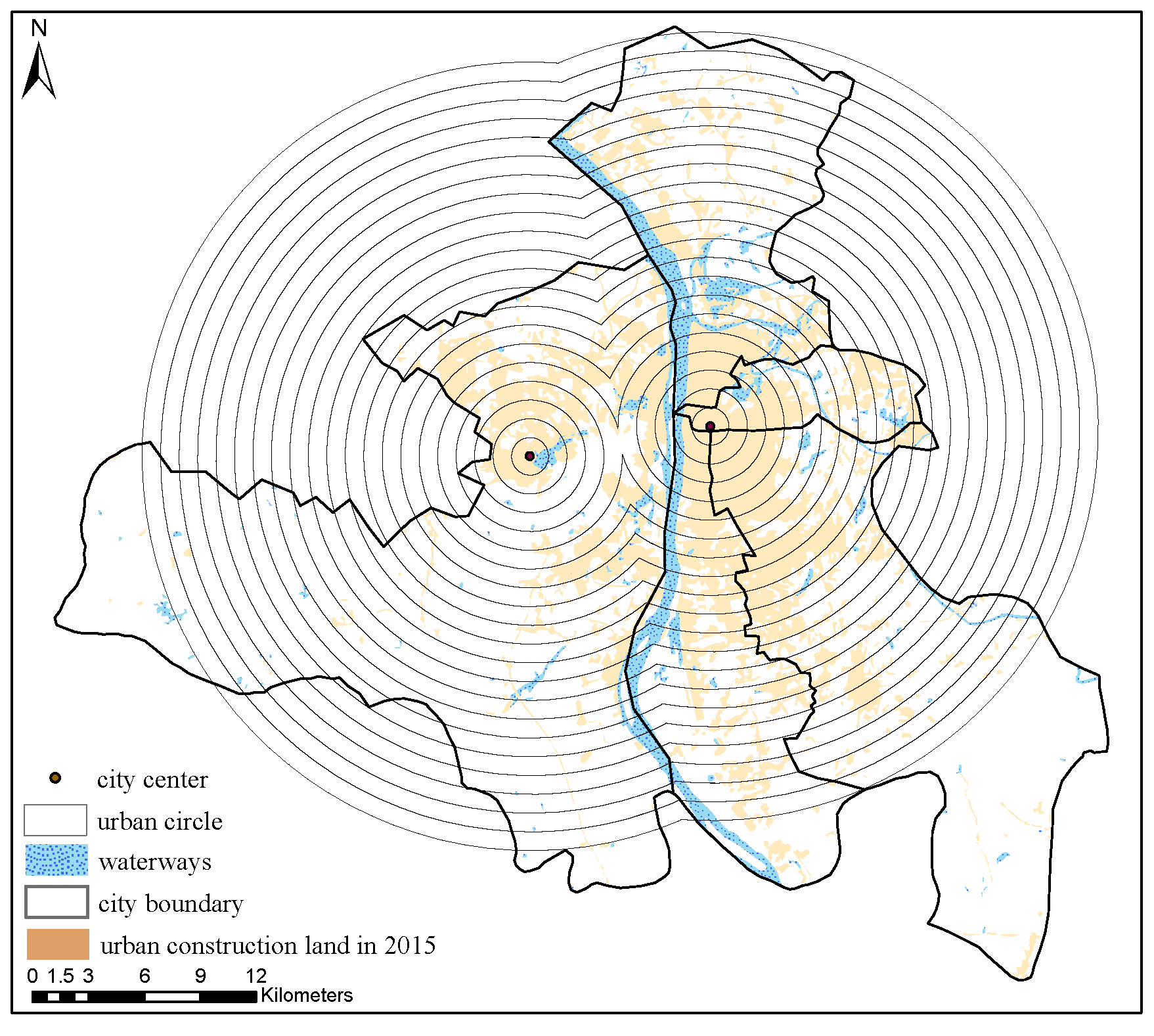
3. Study Area and Datasets

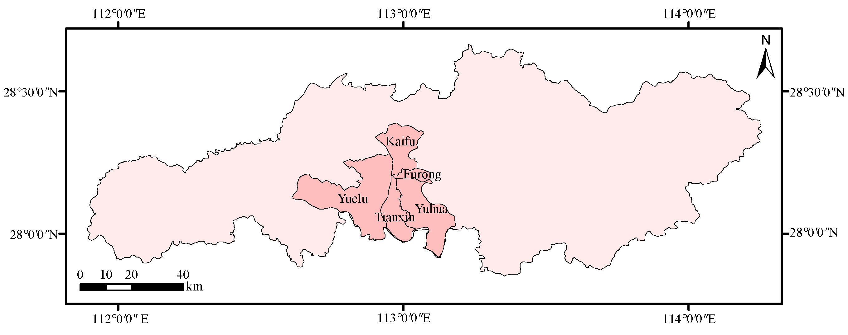
Changsha’s main urban areas, Kaifu, Furong, Tianxin, Yuhua, and Yuelu districts were selected as the study area to verify the validity of the method. The main urban areas, with a total area of 1206 km${}^2$, have the most developed transportation network and highest level of economic development in Changsha. They have high levels of urbanization and a per capita GDP of more than $20,000, and can represent the urban development area of Changsha City. These developed regions have clear urban structures and well-defined functions; therefore, these five districts were selected as the study area (Figure 6).

Two views of Landsat TM/ETM + images (2005/2010) and one Landsat 8 image (2015) are selected to achieve the LULC data of Changsha. The processing steps include image pre-processing, artificial visual interpretation and accuracy evaluation. Firstly, we perform radiometric correction and geometric correction (the number of control points are more than 50) to reduce radiometric and geometric errors in ENVI 5.1. Multi-band images (red band 4, green band 3, blue band 2 in Landsat 4-5 TM; red band 5, green band 4, blue band 3 in Landsat 8) are extracted and fused into false color images, which can be useful to visually analyze different landscape characteristics. To achieve the images of the study area, the false color images are clipped by the administrative boundary of Changsha. Secondly, the interpretation keys for each land category are established from prior knowledge and the survey information. The clipped false color images are artificially interpreted into cropland, green space, waterways, urban land and unused land based on the interpretation keys in ArcGIS 10.2. Thirdly, 1000 sample points for each land class are randomly selected and the historical remote sensed images with more higher resolutions from Google Earth were employed to evaluate the classification results. The overall classification accuracies were 90.1%, 91.5% and 91.7% in 2005, 2010 and 2015, respectively. Finally, the classified images were converted into vector maps and the urban expansion patches were extracted.

Additionally, the road, waterways, and railroad data for the corresponding years were downloaded from the Open Street Map (OSM). Among them, the road data can be further divided into highways, main roads, streets and other data. Next, calculating the Euclidean distance between the patches and OSM and LULC data using the distance tool to obtain the attribution values of distance to green space, highways, streets, railways, main roads and waterways. Further, the calculation of MAI is programed and implemented based on Python 3.7. In the end, the obtained attribute values are normalized to the maximum and minimum values.

4. Results and Analysis

4.1. Global Characteristics of Urban Expansion

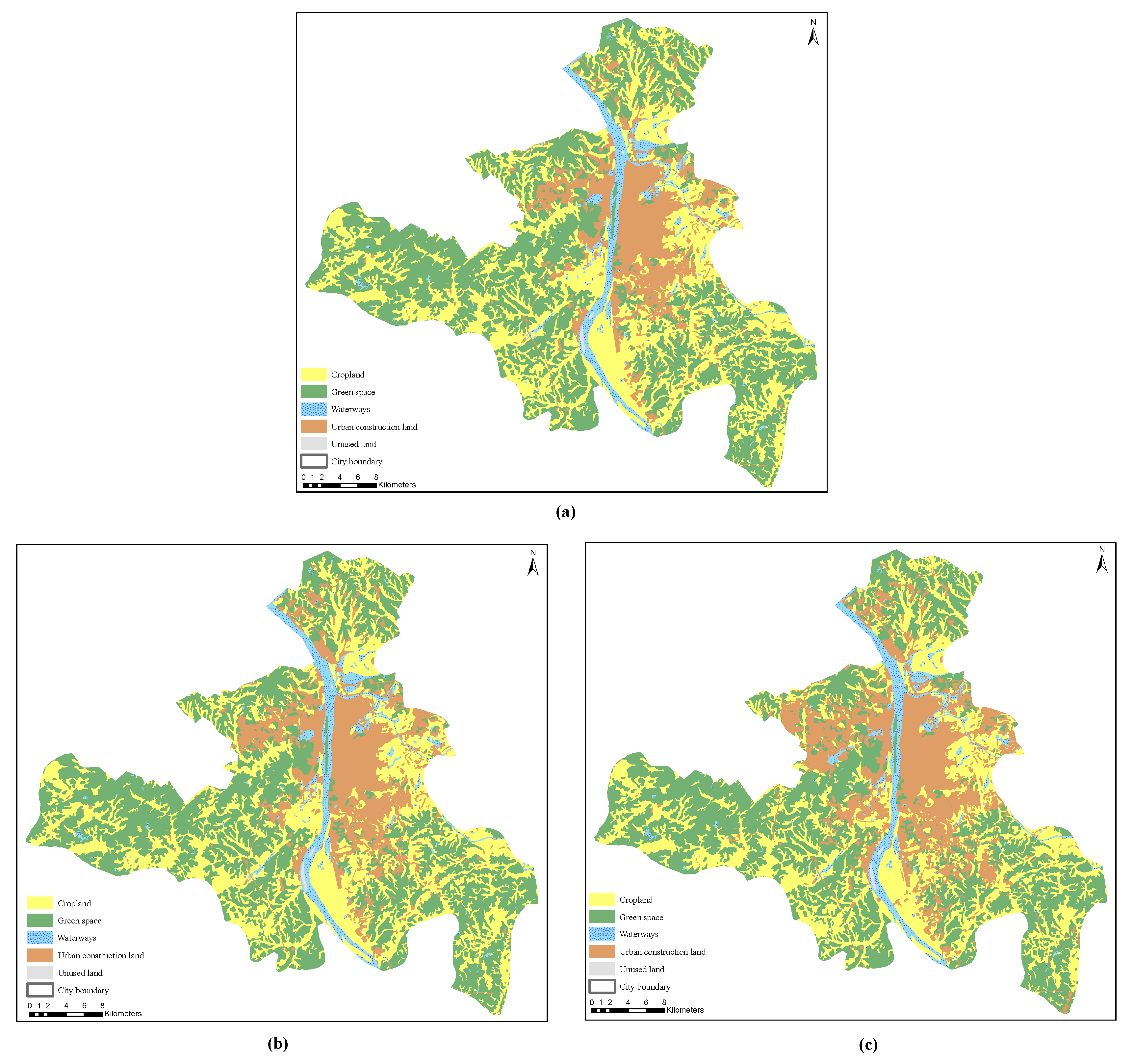
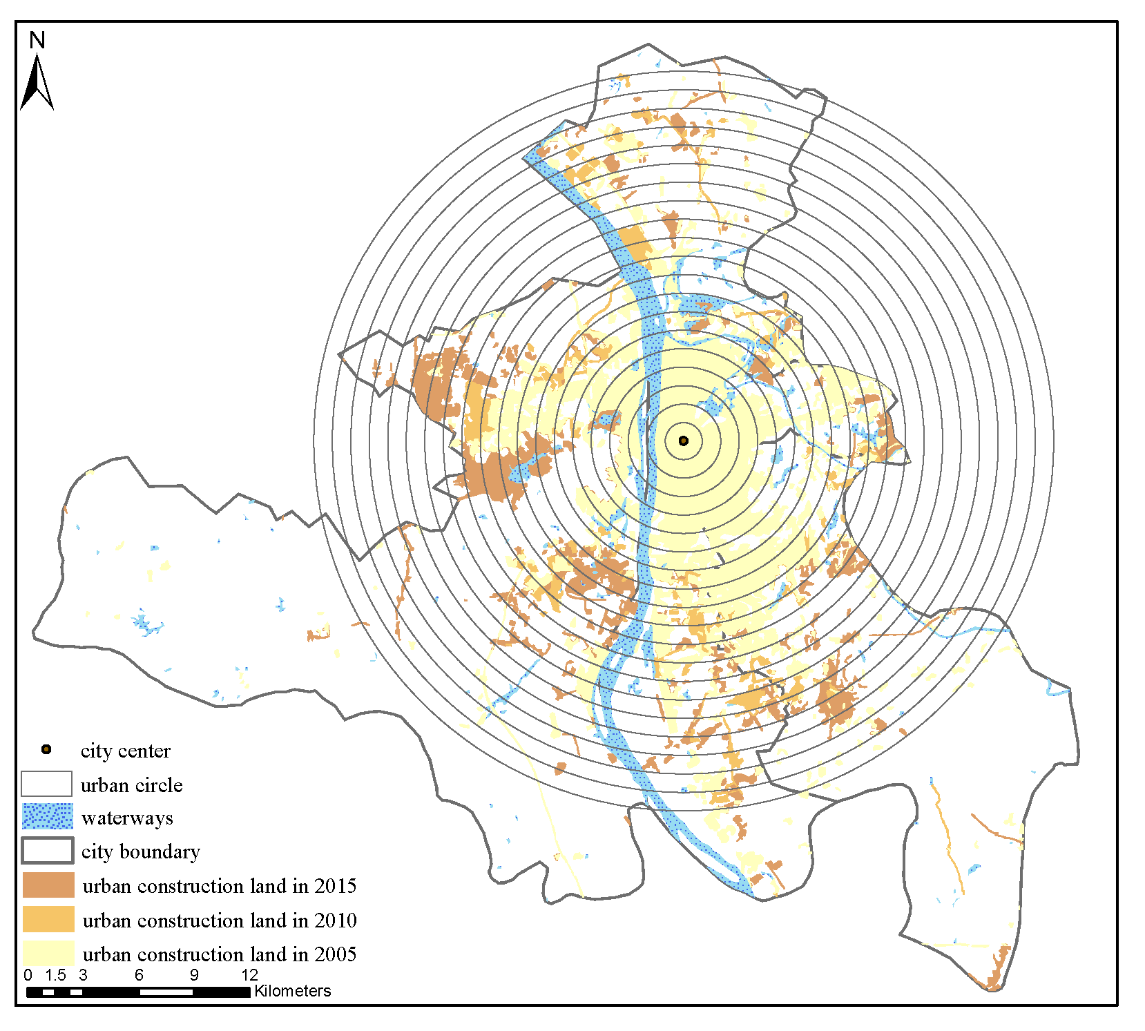
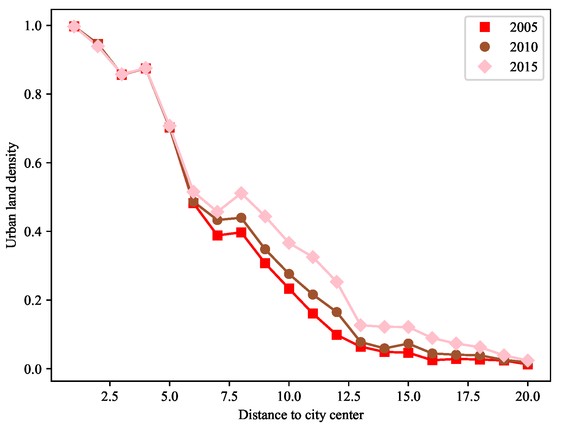
The urban LULC data and circular structures are shown in Figure 7 and Figure 8, respectively. Before 2015, Wuyi Square was the economic center of Changsha City, and using Wuyi Square to represent the center of Changsha City has a certain significance. Changes in the urban land density in 2005, 2010, and 2015 are shown in Figure 9, indicating that the urban land density was high near the center of Wuyi Square, and gradually decreased with increasing distance from the city center. First, the urban land density decreased faster in the front and middle circles. Additionally, the urban land density decreased slowly in the peripheral circles and gradually converged to 0. However, there are two special cases: the fourth and eighth circles. Their urban land densities show a upward trend, which is different from the conventional inverse “S” curve. The reason for this is that there are a large number of water bodies in the third and seventh circles. These water bodies result in the dramatic decline of urban land density in the fourth and eighth circles, which makes the urban land density of the fourth and eighth circles an upward trend.

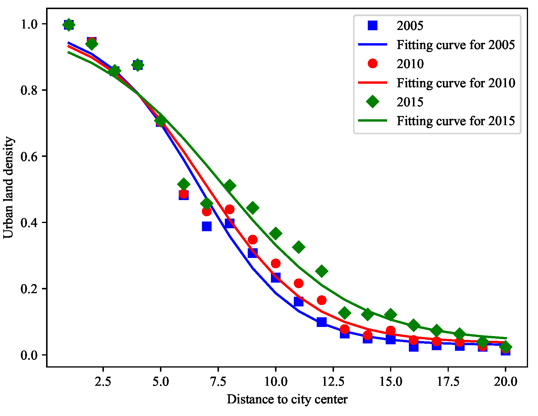
The inverse “S” function was used to fit the urban land density distribution, as shown in Figure 10. The values of inverse “S” are presented in

Table 1. Fitted values of the variables and accuracy of the inverse “S” function in 2005, 2010, and 2015.

Year	a	c	D	${\mathit{R}}^2$
2005	3.24	0.03	13.26	0.94
2010	3.01	0.03	13.87	0.93
2015	2.66	0.04	15.28	0.91

, wherein the function fitting effects $R^2$ were above 0.91 for all three time periods. The fitting parameter D is the result of the estimated radius of the main urban areas, and the values in 2005, 2010, and 2015 are 13.26, 13.87, and 15.28 km, respectively, which indicate that the radius of the main urban areas have expanded with time. The urban land of Changsha was in the diffusion phase during 2005–2015 according to the “diffusion-convergence” urban development phase mentioned in the urban growth phase theory. The estimated increase in the radius of the main urban areas from 2010 to 2015 is 1.41 km; this value is considerably larger than that of the main urban areas, which was 0.61 km from 2005 to 2010. The degree of expansion from 2010 to 2015 was more drastic than that from 2005 to 2010.

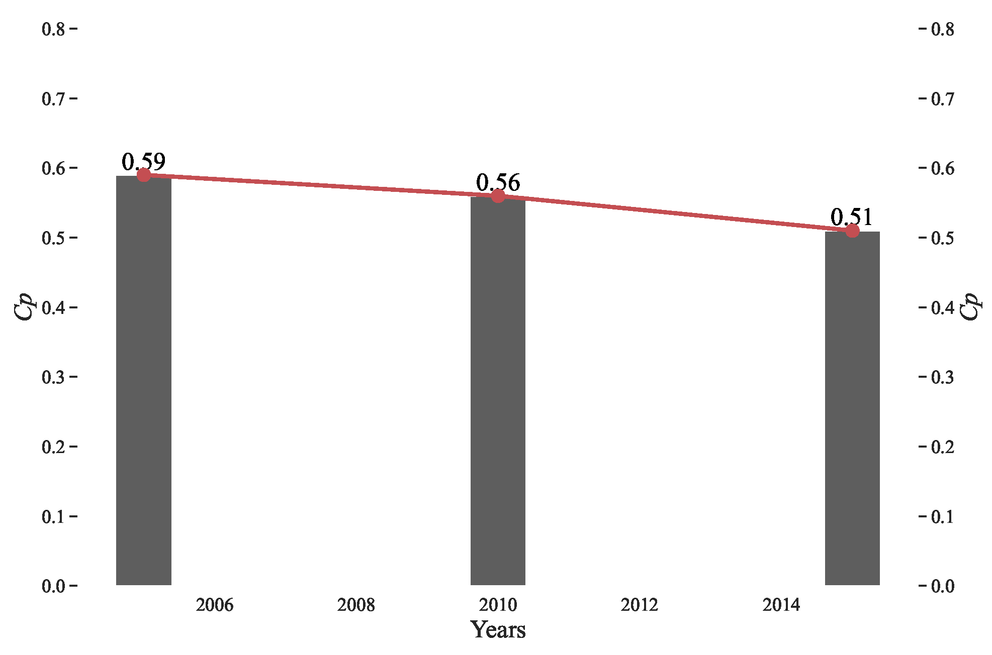
According to the inverse “S” function inversion, the macrocosmic compactness of the city is shown in Figure 11, and the $C_p$ indices for 2005, 2010, and 2015 were 0.59, 0.56, and 0.51, respectively, wherein a larger Cp value indicated a more compact city. Overall, the results show that the urban form became increasingly loose with its expansion, which indicated that the fragmentation of the urban landscape was gradually increasing due to the urban expansion of Changsha from 2005 to 2015.

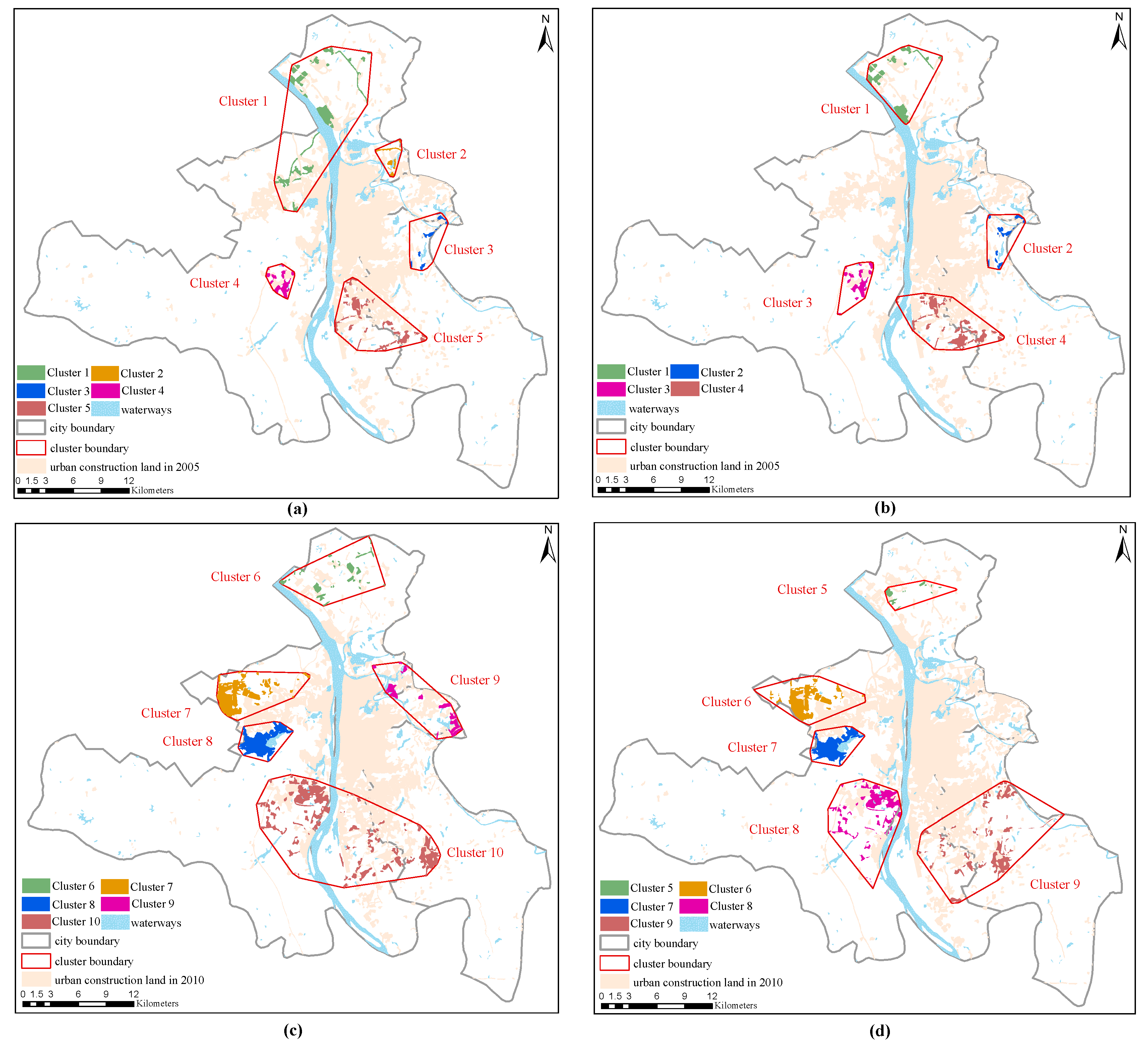
4.2. Urban Agglomeration Characteristics of Expansion Clusters

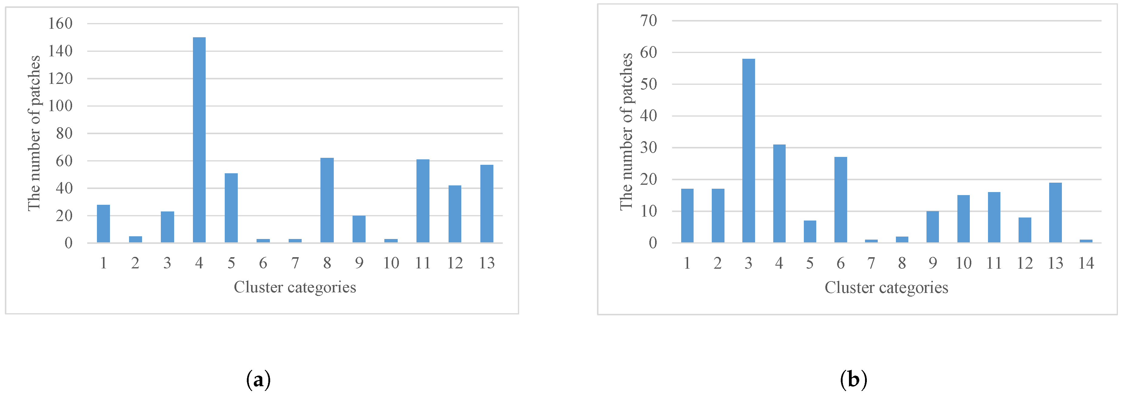
An exhaustive strategy is employed to obtain the optimal urban expansion clusters in the study area. We set three category number thresholds for attribute spatial constraint priority clustering and constraint priority clustering, which are 3, 4, and 5, respectively. Thus, the corresponding dual-clustering result category numbers should be less than or equal to 9, 16, and 25. When the category number threshold is 3, the urban expansion patches in most of the clusters are spatially dispersed. In contrast, when the threshold value is 5, the clustering results are too fine-grained that the adjacent patches are not aggregated into one cluster. As for the result of the category number threshold 4, the clusters are moderate in the spatial continuity and attribute similarity. Therefore, 4 was chosen as the threshold to extract urban agglomeration areas.

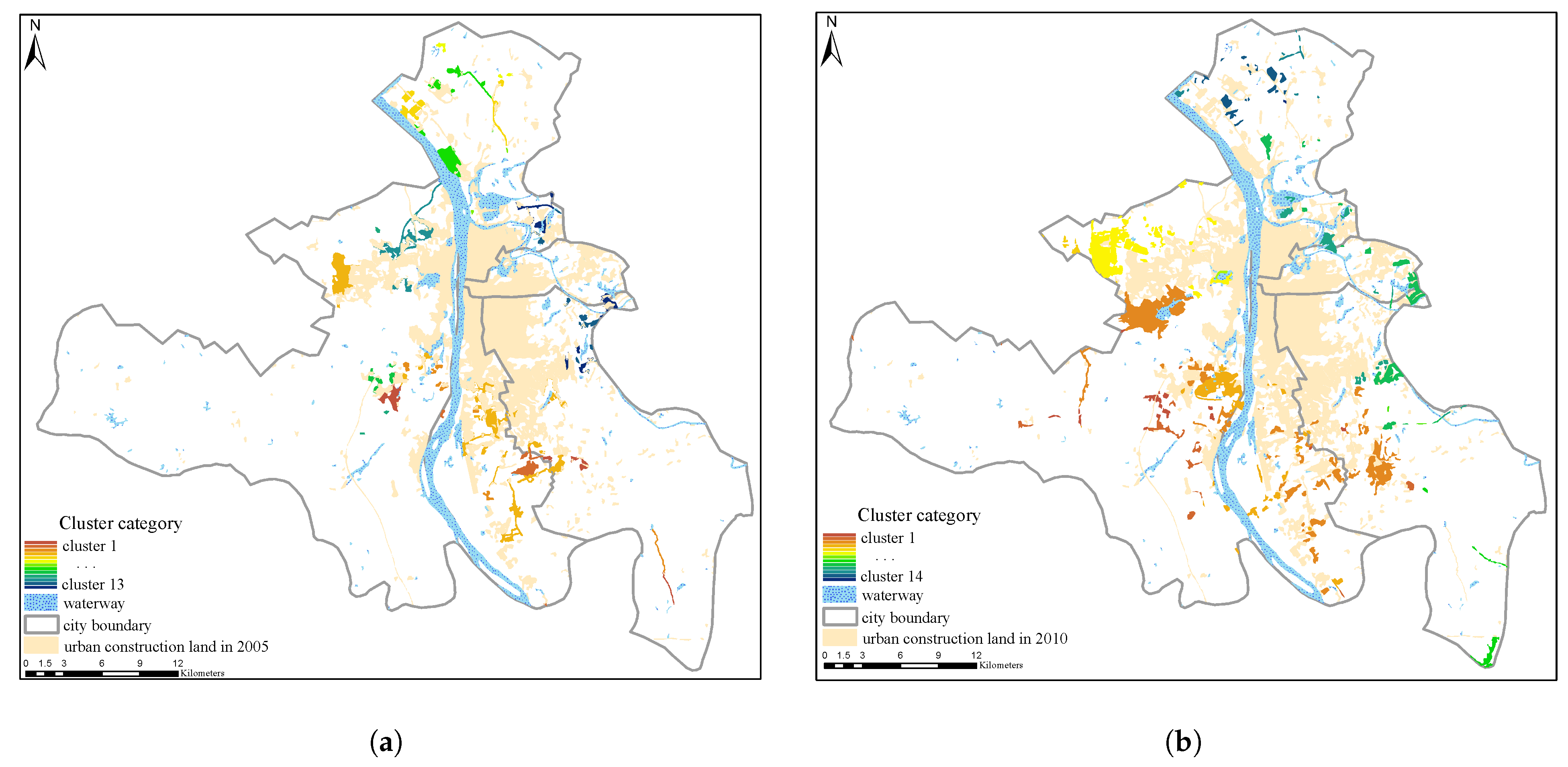
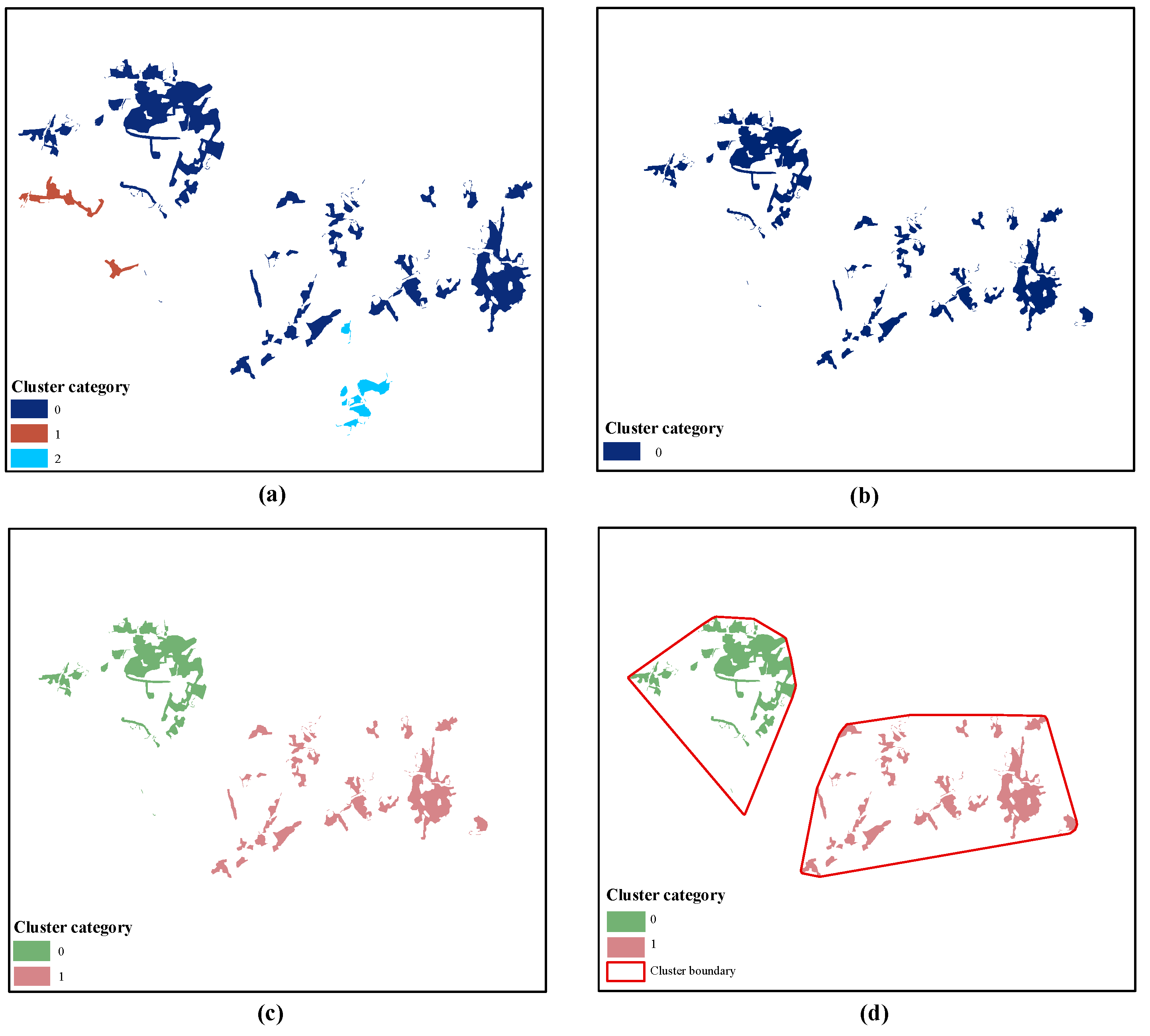
Gaussian mixture dual-clustering model was used to roughly extract urban clusters (Figure 12). As shown in Figure 13, the numbers of patches in Cluster 2, 6, 7 and 10 in 2005–2010 (Figure 13a) and Cluster 5, 7, 8, 12, and 14 in 2010–2015 (Figure 13b) are below 10 and particularly small. By visualizing these clusters (Figure 12), it was found that most of the patches in these clusters are fragmented and loose in the study area, which indicates that these clusters are invalid and need to be removed. By comparing the areas of the expansion patches in the removed clusters, the smallest area of the patches in the large-scale clusters is more than three times the average area of urban sprawl patches. Therefore, 10 was chosen as the constraint threshold for the number of patches and a factor of three times the average patch area was chosen as the constraint threshold for the area of patches.

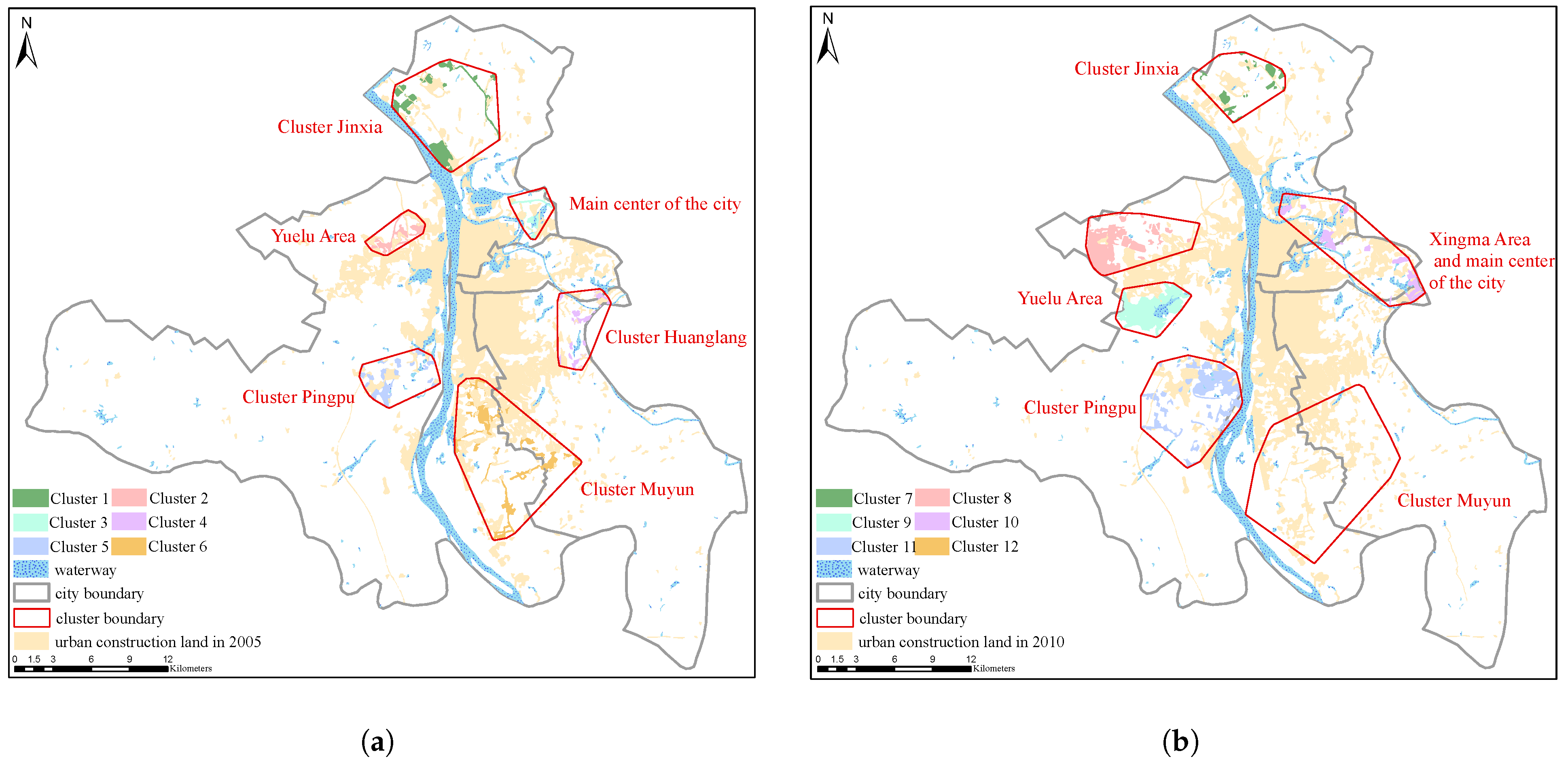
According to experimental results, we found that better results could be obtained if the variable $Minpts$ was within the interval [4, 10]. The results by integrating multi-constraints and the DBSCAN algorithm are shown in Figure 14. Combined with the Changsha City Master Plan (2003–2020) [48] provided by the Changsha Planning & Design Survey Research Institute from 1980 to 2020 (

Table 2. The survey of urban planning and urban planning adjustment in Changsha city from 1990 to 2020.

Planning Time (Year)	Planning of Spatial Structure
1990–2010	One master: Concentrated cluster development area around the old urban land.
	Two wings: Mapoling Quantang (the east wing) and Wangchengpo Tianding Township (the west wing).
	Two clusters: Clusters Laoxia and Pingtang.
1997–2010	Two main bodies: The east and west regions of the Xiangjiang river.
	Three clusters: Clusters Laoxia, Zhanggongling, and Pingtang village.
2003–2020	One main body: The east area of the river.
	Two cities: New city in the west of Xiangjiang river, namely, Xingma new city.
	Four clusters: Clusters Muyun, Laoxia, Gaoxing, and Hanpur.
2003–2020 (revised in 2014)	One axis: The Xiangjiang development axis.
	One main center: The main center of the city is near Wuyi Square.
	Two sub-centers: Yuelu and Xingma sub-centers are located in the Yuelu and Xingma areas.
	Five clusters: Clusters Muyun, Jinxia, Pingpu, Konggang, and Huangli.

), the following results were obtained (based on the final planning period), as shown in Figure 14: Clusters 1 and 7 in (a) and (b), respectively, were located in the Jinxia cluster area; Cluster 2 in (a) and Clusters 8 and 9 in (b) were located in the Yuelu cluster area; Clusters 4 and 11 in (a) and (b), respectively, were located in the Pingpu cluster area; and Clusters 6 and 12 in (a) and (b), respectively, were located in the whole Muyun cluster area and the lower part of the main urban areas. Overall, we identified all cluster areas and other areas in the urban land of Changsha. As the study area was smaller than the central urban land in the Changsha City Master Plan (2003–2020) [48], Cluster 10 showed some errors, but this study still identified the Xingma area.

4.3. Heterogeneous Characteristics of Expansion Clusters

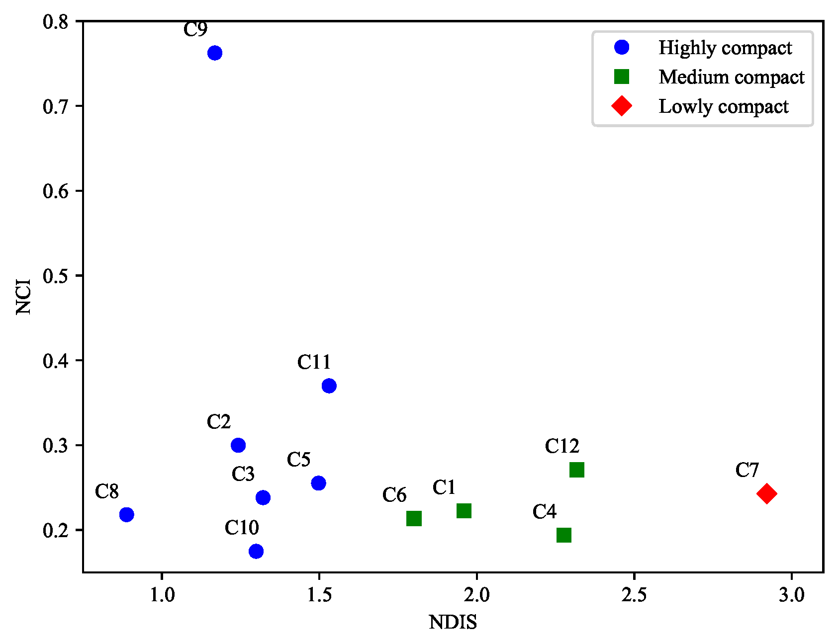
The NCI and NDIS values within the clusters were calculated to determine the compactness of the grouping process. Owing to the large area of patches within Cluster 9, there were only two patches within Cluster 9. Thus, the patches with the largest areas were divided into three parts with equal areas to satisfy the condition of constructing a standard square. A larger NDIS value implies more discreteness, a larger NCI value implies more compactness, and a larger NDIS value implies a smaller NCI value. However, as presented in

Table 3. The results of NDIS and NCI in different clusters.

Years	Cluster ID	NDIS	NCI
2005–2010	1	1.959	0.222
	2	1.242	0.300
	3	1.321	0.238
	4	2.277	0.194
	5	1.497	0.255
	6	1.800	0.214
2010–2015	7	2.921	0.243
	8	0.888	0.218
	9	1.168	0.762
	10	1.299	0.175
	11	1.531	0.370
	12	2.317	0.271

, some differences exist in the rank order of the compact arrangement of some clusters: the highly discrete NDIS has become highly compact at the NCI level. The clusters with small differences are Clusters 1 and 6; the values of Clusters 3 and 5 correspond to the NDIS and NCI values, and the differences are larger for individual clusters, such as Clusters 8 and 10. The differences are mainly reflected in the different logic systems of NDIS and NCI calculations. Although NDIS tends to solve the distance-oriented problem and NCI weighs the influence of urban patch areas on urban compactness, the existence of differences is more conducive to discovering the compactness of urban lands [49].

By combining NDIS and NCI, the identified clusters are classified into three categories using the K-means algorithm: low, medium, and highly compact clusters, as shown in Figure 15. During the first expansion period, the highly compact cluster areas were Clusters 2, 3, and 5, accounting for 50%, and were located in the Yuelu area, main center of the city, and Huangli cluster area, respectively. The Yuelu area is characterized by the presence of scientific research institutes and national high-tech development, where high-tech and modern service industries are concentrated. The main center of the city was in the commercial and business center of Changsha, with compact expansion. The Huangli Cluster area has high-speed railway stations and airports with dense business areas. The medium compact cluster areas were Clusters 1, 4, and 6, accounting for 50%, and were located in the Jinxia, Pingpu, and Muyun cluster areas, respectively. The Jinxia cluster area is located in the transit centers of the urban water transportation, highways, and railroads, with a developed industry. The Pingpu cluster area is characterized by living, residential, and leisure resort areas as it is a university town, whereas the Muyun cluster area was mainly developed for tourism and commerce.

During the second expansion period, some clusters changed significantly, wherein the high, medium, and less compact clusters accounted for 66, 17, and 17%, respectively. First, the highly compact clusters changed more in the Yuelu area; here, the cluster area was located in the eastern part of the Yuelu area from 2005–2010, whereas it was located in the west from 2010–2015 and divided into two clusters. Cluster 9 in the south was the most compact of all clusters, and Cluster 11 in the west was more compact than Cluster 5, which was located in the same cluster area. Owing to less differences in the NDIS index, and by comparison with the NCI index, we found that Cluster 11 was more compact. The last highly compact cluster was located in the main center of the city and Xingma area, which comprised the National Economic Development Zone and Longping High Technology Park with dense high-tech industries. Based on the medium compact clusters, Cluster 12 was located in the same zone as Cluster 6, with a slight deviation in the NCI index. By comparing the NDIS values, we found that Cluster 12 was more discrete. Finally, the industrially developed Cluster 7 was less compact than Cluster 2, with a reduced density of industrial clusters, which is conducive to the construction of a better urban environment.

Through the comparison of compactness and dispersion within the clusters in the two time periods, the visualization results showed that the development of the east-west clusters in the city became more compact, and that of the north-south clusters became looser. The increasingly compact changes in the west fitted into the development strategy of the Changsha City Master Plan (1998–2015) that emphasized the expansion of the west side of the river [50] and compensated for the blank period when the west side of the river was not vigorously developed. The density of the industrial agglomeration in the north decreased, which reduced the emissions of industries and was conducive to the construction of an environmentally friendly city. The south is dominated by tourism development, which can promote urban economic growth, but the urban construction cannot be too loose. A compact city is conducive to sharing resources and infrastructure, reducing the cost of urban operations, and achieving sustainable urban development.

4.4. Analysis of the Offset Characteristics of Urban Clusters

The offset direction and position characteristics are listed in

Table 4. Positional characteristics of clusters in 2005–2010 and 2010–2015 (including circle range, center of gravity position in circle structure (cgpc), and the angle between the centers of gravity of clusters and the direction due north).

Peroid	Cluster ID	Circle Range	Cgpc	Angle (${}^{\circ }$)
2005–2010	1	10–19	14	12.05
	2	6–9	7	54.83
	3	6–9	7	−37.62
	4	6–12	10	137.74
	5	7–20	14	190.99
	6	6–10	8	250.97
2010–2015	7	14–19	17	7.27
	8	7–15	13	74.98
	9	7–13	10	99.43
	10	6–12	8	−66.89
	11	8–16	15	146.46
	12	10–21	11	198.28

and

Table 5. Positional offset characteristics of clusters in 2010–2015.

Cluster ID	CGCI	CGAI (${}^{\circ }$)
7	3	−4.78
8	6	20.15
9	None	None
10	None	None
11	1	−44.53
12	3	−52.69

. By comparing the cluster center of gravity offset, the differences in angles showed that Clusters 8, 11, and 12 shifted to the west from 2010 to 2015. The center of gravity of Cluster 8 was located in the second quadrant of the Cartesian coordinate system of the city center, moving three circles outwards and 20.15${}^{\circ }$ to the $-X$ axis. The center of gravity of Cluster 11 shifted from the fourth to the third quadrant, shifted by 44.53${}^{\circ }$, and moved one circle outward. The center of gravity of Cluster 12 was in the fourth quadrant, deviated from the initial $+X$ axis to the $-Y$ axis, and the deflection angle was 52.69${}^{\circ }$. Clusters 9 and 10 were located in the western marginal area, and the western part of the city affected all five clusters. In the above results, the inverse “S” curve was used to fit the overall land density of the city, and the fitting effect $R^2$ was between 0.91 and 0.93, and did not reach 0.95. Through the above cluster offset and the inverse “S” curve fitting effect, we found that in 2015, urban development might have been affected by other centers. A new urban center might appear in the western region of the city, and the location of the sub-center will be located in the most compact area, namely the 9th location.

5. Discussion

5.1. Comparison of the Effects with Different Attribute Elements

In the above experiment, we used seven-dimensional attribute sets as the input layer of “attribute constraints”, and the weight of each set was equal. In order to verify the importance of the attribute elements for the extraction of urban agglomeration areas, the attribute elements would added into the dual-clustering model one by one. We selected the MAI and the distance to highways as the input layer of “attribute constraints” respectively. MAI was chosen because previous studies have shown significant results when extracting city clusters using MAI [32]. The choice is randomly selected from the six natural and traffic elements because the weight difference of the information entropy model of these six types is not very large [36], and random selection can represent the six types of individua elements.

The results are shown in Figure 16. On the one hand, the experimental results using MAI and the distance to highways are similar to those combining the seven-dimensional attributes. The results of clustering in Figure 16 are roughly located in the clustering and central areas of the Changsha city Master Plan (2003–2020) [48], and none of the clustering areas are located in other areas. Areas 3, 4, 7, and 8 using the MAI and Areas 2, 3, 6, and 7 using the expressway distance elements to form clusters had the same location and similar contours, indicating that the similarities of MAI are similar to those of the distance to highways in these areas, and differences in the distance similarity are not large.

However, the experimental structures obtained using different elements exhibited strong differences, which were embodied in the differences in location and contour lines. The experimental results obtained using the distance element of the expressway (Figure 16b,d) indicated that due to the similarity of the attribute characteristics, some clustering results were unrecognized. Some of the clustering results were also unreasonable, such as those in Cluster 4, wherein both sides of the river were contained in the area. The experimental results obtained using the MAI elements (a and c in Figure 16) indicated that although each location of the cluster was covered, some of the clusters are not refined adequately, such as Clusters 1 and 10, occupying the location of two clusters. Without separation, if this study continues to use algorithm iteration, many fragmented clusters will be generated, destroying the structure of the cluster.

From this experiment, we found that the use of a single attribute will result in incomplete cluster recognition and an insufficient degree of refinement of clusters. A combination of multiple important elements and mutual restrictions can effectively compensate for such defects. However, methods to combine the various elements and quantify the weights are challenges that this research will continue to explore.

5.2. Comparison of the Curve Fitting Effects of Single and Dual Centers

The choice of the city center area is important when using the inverse “S” curve to fit the land distribution in the urban circle. In many studies, the center area is divided into two categories: single-center and multi-center [43], and choosing the appropriate area will have a better fitting effect. The high degree of compactness of urban Cluster 9 in 2015 indicates that it could be the next sub-center of the city. This study compared the dual and single centers of Wuyi Square from to 2010–2015 to determine whether the central structure of the city changed significantly in 2015.

The dual-center circle layer of the city is shown in Figure 17, and the fitting values are presented in

Table 6. Comparison of the curve fitting effect of the single and dual centers of the urban land in 2015.

Type	a	c	D	${\mathit{R}}^2$
Single center	2.66	0.04	15.28	0.91
Dual center	1.83	0.03	10.16	0.92

. The comparative fitting effect increased by 0.01 from a single center to multiple centers, and the increase was not obvious. Conversely, the a value changed obviously and decreased from 2.66 to 1.83, but it represents the slope of the curve of the control urban land density equation, which has no intuitive implication in expressing the process of urban expansion. Additionally, c is the estimated radius of the main urban areas and the change in its value is not obvious. Finally, the D value is the peripheral urban land, and the estimated radius decreased from 15.28 km in a single center to 10.16 km in the dual center. Notably, the increase did not conform to the process of urban expansion stating that the urban fringe area would be farther away from the main urban areas in the process of urban expansion. The D value is expected to increase with time and become increasingly larger, but the result of the dual-center model is smaller than before, which does not match the logic.

6. Conclusions

This study proposed a comprehensive methodological framework to explore the heterogeneous characteristics of urban agglomeration areas during urban expansion from a macrocosmic and microcosmic perspective. The spatial and attribute characteristics were combined to automatically identify and extract agglomeration areas for urban land expansion patches by integrating Gaussian mixture model considering multiple constraints and DBSCAN. Furthermore, the inverse “S” function, POCIS and two improved indices (NCI and NDIS), were introduced to characterize the heterogeneity in urban expansion.

According to the results, we found that: (1) each cluster area and other areas had been identified in the urban land; their recognition rates were high and the final clusters did not contain sparse and broken, small clusters. (2) The analysis of the urban structure indicated that the radius of the main urban areas increased consistently between 2005 and 2015. The city was in the “diffusion” phase and its macrocosmic compactness had continuously declined. The development of the city deviated from the Changsha City Master Plan (2003–2020) [48], which aimed to guide the construction of a compact expansion model. (3) In terms of the microcosmic perspectives, we found that the clusters in the east-west direction of urban expansion were highly compact in the two time periods, and those in the north-south direction were relatively discrete. With the passage of time, the east-west clusters became more compact, and the north-south clusters became increasingly dispersed. Using the cluster migration feature, we found that most urban clusters shifted to the west of the city, which was greatly affected by the west, and the future urban center was likely to appear in Cluster 9.

By comparing the effects of different attribute elements on the experimental results, we found that multi-dimensional attributes produced better model results relative to the single-dimensional attributes. This indicated that the selected attribute data satisfactorily characterized the features influencing the urban patch growth. By comparing the two revised versions of the Changsha City Master Plan (2003–2020) [48], we found that the initial version of the planned city adopted a dual-center structure expansion. During the urban expansion process from 2005 to 2010, Cluster 2, identified by the algorithm, was located in this location and belonged to the highly compact cluster area. However, in the subsequent clustering process, Cluster 2 did not continue to develop, and the southwest part formed a highly compact cluster, which would gradually develop into a sub-center of the city; however, in 2015, it had not yet developed into a sub-center. This change was also in accordance with the revised plan for 2014, which proved that the use of the Gaussian mixture model and the integrated multiple constraints and DBSCAN algorithm in this study were highly effective in the extraction of urban clusters.

This study has the following limitations: (1) the selected urban lands are smaller than the planned areas in the overall plan, leading to the insufficient accuracy of Cluster 10 in 2010–2015. (2) The use of the Gaussian mixture model algorithm and the integrated multi-constraints and DBSCAN algorithm was only applied to one research area, and its application in multiple research areas was not discussed. In future studies, more attributes should be combined, and this method should be applied to other research areas to determine the common features of the iterative recognition algorithm among cities. Additionally, generalizing the algorithm for extracting urban structural features and identifying the process of urban expansion would be worthwhile in the future.