Article

Estimating Layered Cloud Cover from Geostationary Satellite Radiometric Measurements: A Novel Method and Its Application

1
College of Meteorology and Oceanography, National University of Defense Technology, Changsha 410073, China
2
Key Laboratory for Atmosphere and Global Environment Observation, Chinese Academy of Sciences, Beijing 100029, China
*
Author to whom correspondence should be addressed.
These authors contributed equally to this work.
Remote Sens. 2022, 14(22), 5693; https://0-doi-org.brum.beds.ac.uk/10.3390/rs14225693
Submission received: 22 September 2022 / Revised: 5 November 2022 / Accepted: 7 November 2022 / Published: 11 November 2022
(This article belongs to the Special Issue Satellite-Based Cloud Climatologies)

Abstract

:
Layered cloud cover (LCC), that is, cloud cover at different levels, is crucial for estimating cloud radiative effects and modeling climate change. However, accurate LCC characterization using passive satellite measurements is challenging because of the difficulties in resolving cloud vertical structures. In this study, we developed a novel method to estimate LCC from geostationary satellite radiometric measurements. The proposed method resolves cloud vertical structures by retrieving cloud-top and cloud-base heights for both single- and multi-layer clouds; thus, better estimating LCC. Our results agreed well with active satellite measurements, showing identification accuracies of 86%, 90%, and 91% for high, medium, and low clouds, respectively. Additionally, our LCC estimates derived from satellite measurements were used to evaluate those from atmospheric reanalysis. The annual averaged total, high, medium, and low cloud covers given by our methods were 0.681, 0.393, 0.356, and 0.455, respectively, while those from ERA-5 were 0.623, 0.415, 0.274, and 0.392, respectively. These results indicate that the total cloud cover determined by ERA-5 was lower than that derived from satellite measurements, potentially as a result of medium and low-level clouds.

1. Introduction

Clouds are crucial to the radiation balance of the Earth–atmosphere system, but their radiative effects strongly depend on cloud cover, cloud height, cloud phase, and vertical cloud overlap [1,2,3]. Cloud cover represents the amount and horizontal distribution of clouds, and determines the area affected by clouds [4,5], while cloud height reflects the vertical distribution of clouds, affecting their capability to modulate incoming shortwave and outgoing longwave radiations [6]. As shown in Figure 1, low clouds generally cause an atmospheric cooling effect due to strong outgoing longwave infrared radiation and strong reflectance of incoming solar radiation, while high clouds emit less longwave infrared radiation and reflect less incoming solar radiation, leading to atmospheric warming [3,7]. Therefore, cloud cover at different levels, that is, layered cloud cover (LCC), is important to evaluate cloud radiative effects [5,6].
Many studies have investigated climate change with LCC simulations from general circulation models (GCMs) [8,9,10]. Randall et al. [11] demonstrated that the atmospheric cooling effect caused by a 4% increase in global marine low cloud cover would result in a 2–3 K decline in global temperature. Climate models have been reported to capture seasonal variations of the surface total radiative flux in Arctic regions only when cloud cover was accurately simulated [12]. Global cloud measurements and simulations to demonstrate that clouds exhibit positive feedback [6]; however, considerable LCC simulation deviations exist between different climate models, resulting in large prediction uncertainties regarding future climate change [5,13]. To narrow these inter-model differences, previous studies have used ground-based instruments, such as visible all-sky cameras and ceilometers, to evaluate LCC simulations using GCMs; however, while ground-based instruments provide accurate LCC measurements, their observational coverage is limited and they cannot be employed for global evaluation. Thus, there is a need for continuous LCC measurements from satellite remote sensing to understand the spatiotemporal distribution of clouds and evaluate LCC simulations from GCMs.
Geostationary (GEO) satellites are powerful tools for continuous cloud observation because of their wide observational coverage and high spatiotemporal resolutions [14]. The accurate estimate of LCC requires reliable information concerning cloud vertical structures, such as cloud top height (CTH), cloud base height (CBH), and cloud thickness. Since visible and infrared wavelengths can hardly penetrate clouds, especially thick ones, satellite radiometer measurements are primarily determined by spectral signals from the cloud tops of the uppermost cloud layer and contain limited information regarding cloud vertical structures [15]. Consequently, while CTH has been provided as a fundamental cloud property product for many years [16,17], retrieving CBH is still a challenge [18,19]. Moreover, most satellite cloud property products (e.g., CTH) are generated based on single-layer cloud assumptions, leading to large retrieval errors in multi-layer cloud systems [20,21]. These problems in the CTH and CBH retrievals clearly limit the estimation of LCC. Currently, most satellite cloud cover products are generated based on cloud detection, which reflects only the total cloud cover (TCC) observed from space [22]. By introducing CTH retrievals, conventional TCC data has been improved into LCC data based on measurements from the Geostationary Operational Environmental Satellites (GOES-R) [16]; however, cloud vertical structures have not been fully characterized because of the lack of critical CBH information and CTH biases in multi-layer cloud cases, leading to large LCC estimate uncertainties.
Previous studies have used satellite-retrieved total cloud cover to evaluate those from atmospheric reanalysis, but cloud vertical structures have been rarely considered [23]. An evaluation using LCC estimates from satellite measurements can help to better understand the performance of atmospheric reanalysis. Recently, we developed a CBH estimation and multi-layer CTH extrapolation algorithm [24,25,26]. These algorithms further improved the capability of passive radiometers in resolving cloud vertical structures by providing critical CBH information and reducing CTH retrieval errors in multilayer cloud cases. It implies that cloud vertical structures could be better characterized using GEO satellite measurements. However, whether these advances in cloud height retrieval algorithms could be used to improve the estimate of LCC has not been studied.
In this study, we provide a novel method for inferring LCC from GEO satellite radiometric measurements and evaluate the LCC given by ERA-5. The paper is organized as follows. The LCC estimation method is described in Section 2 and is validated using active satellite measurements in Section 3. Section 4 evaluates the LCC derived from ERA-5 based on long-term GEO satellite measurements. A brief summary of the paper is presented in Section 5.

2. Data Sets and Method

2.1. Data Sets

Himawari-8, one of the most advanced GEO satellites, is considered a representative GEO satellite in this study [14,27,28]. The LCC includes high, medium, and low cloud cover, which are distinguished by cloud heights. Following the definition of the European Center for Medium-Range Weather Forecasts (ECMWF), high, medium, and low cloud cover were defined as the proportion of a grid box covered by clouds occurring in the high, medium, and low levels of the troposphere, respectively [29]; therefore, knowledge of cloud boundaries, such as CTH and CBH, is critical for estimating LCC.
Similar to most satellite cloud products, the Advanced Himawari Imager (AHI) onboard Himawari-8 provides CTH retrievals generated based on single-layer cloud assumptions but does not include CBH as one of its cloud property products; hence, CTH retrievals typically perform well for single-layer clouds but may be heavily biased in the case of multi-layer clouds [30]. To estimate the LCC, we retrieved CBH data and improved the multi-layer cloud height AHI measurements. Figure 2 shows the workflow of this novel LCC estimation algorithm, which includes three main steps: (1) CTH and CBH retrieval for single- and multi-layer clouds, respectively; (2) high, medium, and low cloud classifications for each cloudy pixel with available CTP (cloud top pressure) and CBP (cloud base pressure) retrievals; and (3) high, medium, and low cloud cover calculations, respectively. The green boxes in Figure 2 denote the input satellite measurements (i.e., the AHI L1b and L2 CLP products), the blue boxes represent the intermediate variables (i.e., multi-layer cloud detection, CTH, and CBH retrievals), and the yellow boxes represent the desired LCC results, including high, medium, and low cloud cover.
The AHI level-1b (L1b) and level-2 CLP (L2 CLP) products during 2015 and 2017 were used for the analysis of LCC climatology. Additionally, the ECMWF Reanalysis version 5 (ERA-5) data were used to convert the CTH and CBH retrievals to cloud top pressure (CTP) and cloud base pressure (CBP), and the LCC from ERA-5 was compared with our results. The combined measurements of the Cloud Profiling Radar (CPR) on-board CloudSat and the Cloud–Aerosol Lidar with Orthogonal Polarization (CALIOP) onboard the Cloud–Aerosol Lidar and Infrared Pathfinder Satellite Observation (CALIPSO) satellite provide well-recognized vertical cloud structure measurements [31,32,33]. Hence, 2B-CLDCLASS-LIDAR, a CPR-CALIOP combined product, was used for the algorithm validation.

2.2. Layered Cloud Cover Estimation Method

2.2.1. Retrieval of CTH and CBH

Accurate and complete vertical cloud structure characterization using only radiometric measurements is a challenging task, primarily because of the strong absorption of spectral signals by clouds. Unlike existing methods, this algorithm combined conventional radiative transfer model-based (physics-based), machine-learning-based (ML-based), and statistical extrapolation-based (SE-based) methods to overcome these limitations. As shown in Figure 3, cloud vertical structures could not be sufficiently characterized by conventional single-layer-based CTH retrievals, but could be better inferred by considering CTH and CBH retrievals for both single- and multi-layer clouds.
First, the ML-based multi-layer cloud detection algorithm proposed by [25] was used to distinguish multi-layer clouds from single-layer clouds because the retrieval methodology for multi-layer clouds differs from that of single-layer clouds. Owing to the advantage of the cloud sensitivity channels (e.g., 2.25 μm) equipped with the AHI and the powerful performance of machine learning techniques on nonlinear classification tasks, this multi-layer cloud detection algorithm outperformed conventional physical methods (e.g., MODIS products). Moreover, the algorithm is adept at labeling multi-layer clouds with large retrieval errors, which is critical for the improvement of multi-layer CTH and CBH retrievals.
Subsequently, single-layer CTH retrievals were directly extracted from AHI L2 CLP, which was produced via physics-based methods by assuming that all the clouds are single-layered and homogeneous [30]. Direct CBH retrieval is theoretically difficult for passive radiometers, such as AHI, because radiometric measurements contain limited information about the cloud base. Many existing methods infer CBH by subtracting the cloud geometric thickness (CGT) from mature satellite-retrieved CTH data, where the CGT is estimated using cloud microphysical and optical properties. Here, the ML-based CBH estimation algorithm proposed by [24] was chosen as it could accurately estimate CBH by considering conventional cloud microphysical and optical properties, as well as environmental factors. However, the main inputs and cloud optical and microphysical properties were retrieved from radiometric measurements in the visible and near-infrared spectral channels [24]. Thus, CBH retrieval can only be conducted for daytime measurements, which is a common limitation of CBH retrieval from passive radiometers.
For multi-layer cloud systems, we considered the SE-based algorithm proposed by [26]. Multi-layer clouds are common in the atmosphere and account for over 25% of global clouds. Since radiometric measurements do not accurately represent the spectral signals of any individual cloud layer in multi-layer cloud cases, it is difficult to retrieve cloud properties from these complex cloud systems using conventional physics-based methods [15,34]. Consequently, multi-layer cloud height information has not been considered in existing satellite cloud cover products. The extrapolation algorithm takes advantage of cloud continuity and assumes that local cloud boundaries are similar. Hence, multi-layer cloud heights can be inferred from the neighboring single-layer cloud heights. All multi-layer clouds are treated as cases where ice clouds overlap water clouds, which are the most common type of multi-layer clouds. Three physical constraints (cloud phase, neighboring, and cloud optical thickness) were developed to minimize the uncertainties in the extrapolation process. Once multi-layer clouds are detected, the upper-layer ice CTH/CBH are inferred using the known single-layer CTH/CBH of neighboring ice clouds, and the lower-layer water CTH/CBH are inferred using the known single-layer CTH/CBH of neighboring water clouds. Moreover, the algorithm is performed without radiative transfer simulations; thus, its computational efficiency is much higher than that of the conventional physics-based retrieval methods [34]. The input variables for multi-layer cloud detection, CBH estimation, and multi-layer cloud extrapolation are summarized in Table 1.

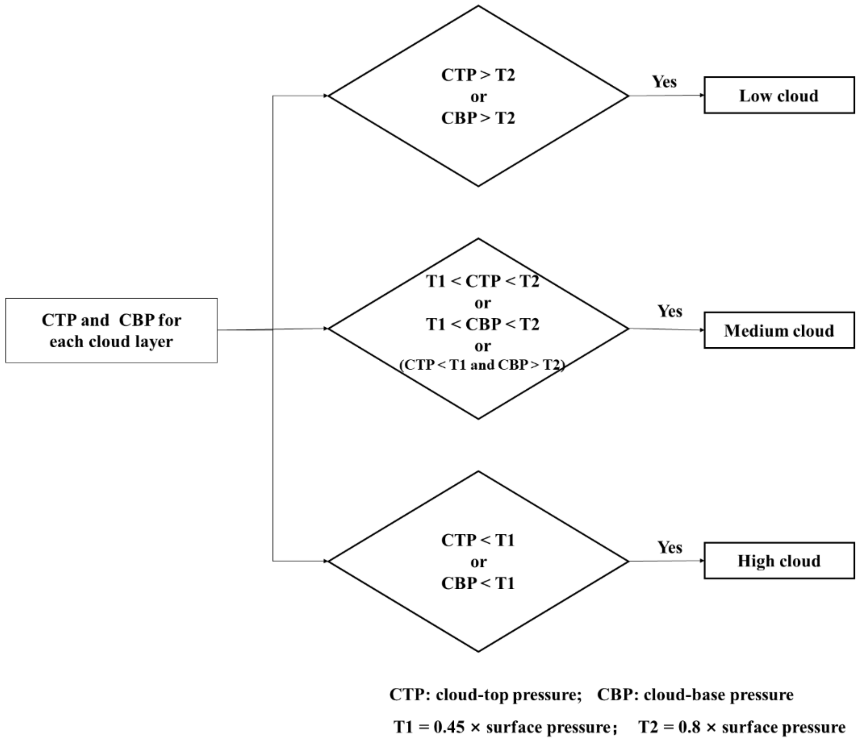
2.2.2. Classification of High, Medium, and Low Clouds

With the vertical distribution of clouds represented by CTH and CBH retrievals, high, medium, and low-level cloud occurrences were determined. First, CTH and CBH retrievals were converted to CTP and CBP using ERA-5 data. Then, we determined the presence of high, medium, and low clouds for each cloudy pixel based on CTP and CBP. The decision flowchart is illustrated in Figure 4. The layer thresholds for differentiating high, medium, and low clouds were 0.45 times and 0.8 times the surface pressure [29]. For example, if a single-layer cloud pixel had a CTP of 430 hPa, a CBP of 830 hPa, and a surface pressure of 1000 hPa, clouds were recognized at all three levels (low level: 1000–800 hPa; medium level: 800–450 hPa; high level: >450 hPa). If a multi-layer cloud pixel had an upper-layer CTP/CBP of 330 hPa/440 hPa and a lower-layer CTP/CBP of 900 hPa/950 hPa, only high and low clouds were identified. Pixel-level (0.05° × 0.05°) cloud-type identification was conducted for all cloudy pixels with available CTPs and CBPs.

2.2.3. Calculation of LCC

Finally, pixel-level cloud type identifications were used to calculate the proportion of a 5 × 5-pixel box covered by high, medium, and low-level clouds, respectively. In this way, we obtained cloud cover estimates at high, medium, and low levels, ranging from 0 to 1. Notably, this study focused on daytime LCC estimations because of its dependency on visible and near-infrared spectral measurements. Our LCC spatial resolution (0.25° × 0.25°) was consistent with that of ERA-5, while our results were derived from atmospheric measurements and could be provided in near real-time with a high temporal resolution of 10 minutes.

3. Validation Using Active CPR-CALIOP Data

Before the evaluation of LCC derived from reanalysis data, we need to validate the algorithm’s performance. Here, we compared the LCC estimates derived from AHI measurements with those from the 2B-CLDCLASS-LIDAR product. While 2B-CLDCLAS-LIDAR provides well-recognized measurements of cloud vertical structures, it covers only nadir pixels along the satellite tracks and cannot be used to calculate the LCC. Therefore, evaluation was performed for pixel-level cloud classification, that is, high, medium, and low clouds. This evaluation was equal to that of LCC because LCC was directly calculated with pixel-level cloud classification.
An example of LCC estimates from AHI measurements at UTC 07:00 on October 5, 2017, is presented in the above figures. Figure 5 shows the multi-layer cloud detection results. Clouds covered over 60% of the selected region (80°E–142°E, 5°S–60°S), and approximately 20% of them were identified as multi-layered. Figure 6a,b shows the upper-layer CTH and CBH retrievals, respectively. For pixels identified as multi-layer clouds, our method would further generate estimates of lower-layer CTH and CBH in Figure 6c,d. Thus, a three-dimensional cloud field was established to better understand the spatial distribution of clouds. Figure 7a–c shows the high, medium, and low cloud cover estimates, which may benefit the estimation of cloud radiative forcing by separately considering the radiative effects of clouds at different levels. Figure 7d,e shows a cross-section comparison between the active CPR-CALIOP measurements and AHI results, corresponding to the satellite tracks marked by black lines in Figure 7a–c. Although passive radiometers, such as AHI, have natural limitations in retrieving cloud vertical structures, our algorithm produced reasonable estimates of three-dimensional cloud fields. The vertical distributions of clouds determined by our CTH and CBH retrievals were close to those of the active CPR-CALIOP measurements. As a result, the cloud type classifications from CPR-CALIOP and AHI were mostly consistent, with some disagreements for high clouds.
Another example of LCC estimates was derived from AHI full-disk measurements at UTC 03:00 on 23 September 2021. As shown in Figure 8, the spatial distribution of clouds are clearly described, as 3D cloud structures were obtained by retrieving CTH and CBH for both upper- and lower-layer clouds. the results indicate that high clouds occur more frequently in tropics, whereas medium and low clouds appear to be more common in mid-high latitudes.
Additionally, we conducted a statistical evaluation based on a collocated AHI-CPR-CALIOP dataset, which had approximately 5,300,000 samples derived from strict spatiotemporal matches between the AHI and CPR-CALIOP measurements during 2015 and 2017. To better understand the influences of newly introduced cloud heights information in LCC estimates, we considered two schemes in which the LCCs were estimated with different inputs. Scheme 1 (S-1) used only the CTH retrievals based on the single-layer cloud assumption (i.e., the AHI L2 CLP product), while Scheme 2 (S-2) used the CTH and CBH retrievals of both single- and multi-layer clouds (i.e., our results). Figure 9a shows the percentages of cloud classification results obtained by S-1 and S-2, which agree with the CPR-CALIOP measurements. Since S-1 only considered CTHs, the cloud base boundaries were unknown, leading to an obvious underestimation of medium- and low-level clouds, which had identification accuracies of 64% and 60%, respectively. Moreover, 21% of the high clouds were incorrectly identified, likely due to two major reasons. First, multi-layer CTH retrievals may have been significantly underestimated. Second, the limited sensitivity of AHI to thin high clouds caused some to be overlooked [30]. By introducing the CBH, S-2 significantly improved the identification accuracy of medium and low clouds to 90% and 91%, respectively. Moreover, improved multi-layer cloud height retrievals from the extrapolation algorithm improved the identification accuracy of high clouds from 79% to 86%.
The annual average fractions of high, medium, and low clouds derived from S-1, S-2, and CPR-CALIOP data are shown in Figure 9b. As expected, S-1 considerably underestimated each cloud type. In particular, S-1 only correctly identified approximately 50% of the low clouds determined by CPR-CALIOP. Since low clouds have been regarded as a major modulator of cloud radiative forcing, this underestimation may substantially affect climate change simulations. However, our algorithm yielded results that were much closer to those obtained from CPR-CALIOP. The cloud fraction differences between S-2 and CPR-CALIOP were −0.03, 0.01, and −0.01 for high, medium, and low clouds, respectively.
Overall, by introducing CBH retrievals and improving multi-layer cloud height retrievals, our methods achieved high-accuracy high, medium, and low cloud classifications comparable to active CPR-CALIOP measurements. However, uncertainties from multilayer cloud and cloud base height estimates also introduce inevitable uncertainties to LCC retrieval. For multi-layer clouds, the extrapolation method assumes all multi-layer clouds to be ice-over-water clouds. Thus, the estimated CTH and CBH may be less accurate in cases where more complicated multi-layer cloud systems (e.g., three-layer cloud) exist, leading to more uncertainties in the LCC retrieval. For cloud base height, due to the sensitivity limitation of AHI, clouds with small COT may have larger CBH retrieval errors. Consequently, the LCC estimates may also be affected in cases of optically thin clouds, for example, thin cirrus. Nevertheless, the application of the proposed algorithm in GEO satellite systems enables high spatiotemporal resolutions, continuous, and large-scale LCC estimates, which would be valuable for better understanding the spatiotemporal distribution of clouds and could be used to evaluate LCC from atmospheric reanalysis as well as GCMs.

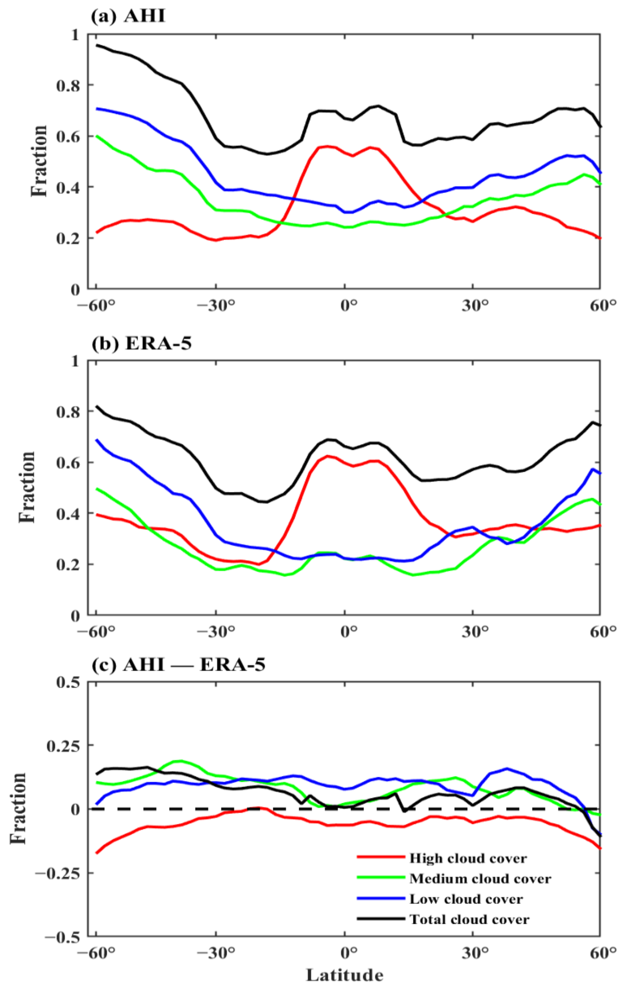
4. Comparison of LCC between AHI and ERA-5

Combining various sensor observations and simulations from different numerical models, atmospheric reanalysis is a powerful means of representing atmospheric temperature and moisture, clouds, precipitation and rain, radiation, etc. Owing to the difficulty of assimilating cloud observations in reanalysis, most cloud properties, including cloud cover, are produced via cloud parameterization schemes. Therefore, knowledge of the differences between atmospheric reanalysis and actual observations is indispensable to weather and climate studies using reanalysis data. As one of the most advanced reanalysis datasets, ERA-5 has been extensively evaluated using in situ and satellite observations. However, previous comparisons between satellite observations and reanalysis data have predominantly been performed for TCC, ignoring cloud vertical structures [23].
In this study, we compared the LCC estimates derived from AHI observations and those from the ERA-5 reanalysis data. This comparison is particularly meaningful for revealing the performance of ERA-5 in representing the cloud cover at different levels. The AHI and ERA-5 data for all of 2017 were used for comparison, and the study area ranged from 80°E to 160°W and from 60°S to 60°N. Since the AHI LCC estimates were generated based on daytime observations, we only utilized daytime ERA-5 data for comparison. Additionally, the temporal resolution of the ERA-5 reanalysis data was one hour, whereas that of the AHI was 10 min. For a fair comparison, the AHI results were averaged hourly.
Figure 10 shows the annual mean reanalysis- and observation-derived LCC and their differences, respectively. The LCC spatial distributions given by AHI and ERA-5 were in good agreement. Notably, the tropics are covered with high clouds most of the time, as the annual average high cloud cover exceeds 0.8. High cloud cover is smaller in the mid-latitudes and appears to be larger in the Northern Hemisphere than that in the Southern Hemisphere. Geographical variation in medium cloud cover was less significant, approximately 0.3 in most areas, except for the relatively large medium cloud cover (over 0.5) over the southern oceans of Australia. Additionally, low cloud cover is relatively small in the tropics and large in the mid-latitudes. Table 2 lists the annual average TCC and LCC derived from AHI measurements and ERA-5 reanalysis, respectively. The average TCC was 0.623 for ERA-5 and 0.681 for AHI, indicating that the ERA-5 reanalysis data underestimated TCC by 0.058. This finding is similar to that of [23], who suggested that the cloud cover indicated by ERA-5 was approximately 0.06 smaller than that of the Moderate Resolution Imaging Spectroradiometer (MODIS), which is a benchmark of spaceborne passive radiometer. For LCC, the high, medium, and low cloud cover from ERA-5 were 0.415, 0.274, and 0.392, respectively. In contrast, AHI values were 0.393, 0.356, and 0.455, respectively. Therefore, our results further suggest that the underestimation of total cloud cover in the ERA-5 reanalysis may be predominantly attributed to the underestimation of medium and low cloud cover. These findings are also similar to those of [5], who suggested that most climate models overpredict high cloud cover and underestimate medium and low cloud cover when compared with measurements at the United States Southern Great Plains site. However, our evaluation using GEO satellite measurements indicated that the underestimation of medium and low cloud covers by reanalysis may be a common phenomenon, which should be given sincere consideration in future improvement of cloud parameterization schemes.
Figure 11 shows the zonal average of the annual mean LCC and TCC given by AHI and ERA-5. TCC and LCC each varied greatly depending on the latitude as many factors may affect the occurrence and development of clouds, such as atmospheric circulation, surface temperature, and aerosols. The TCC exhibits a peak in the tropics between 15°S and 15°N and becomes relatively small between 15° and 30° in both hemispheres. The largest TCC was found near 60°S, where clouds were nearly always present. When the vertical distribution of clouds was considered, some notable findings concerning the spatial distribution of clouds were obtained. For example, the zonal variation of high cloud cover was similar to that of TCC; in particular, high cloud cover dominated the distribution of TCC in the tropics. In contrast, medium and low cloud cover reached their minimum in the tropics and increased with the latitude in both hemispheres. Referring to the AHI results, Figure 8c indicates that the ERA-5 reanalysis may overpredict high cloud cover, but underestimate medium and low cloud cover. Moreover, the differences between AHI and ERA-5 were significant for mid-latitude regions in the Southern Hemisphere (30°S–60°S).
A distinct advantage of GEO satellites is that they can monitor temporal variations of atmospheric components like clouds. Figure 12 shows the monthly average TCC and LCC from AHI and ERA-5 and their differences. Compared with Figure 11, the temporal variations in both TCC and LCC were not as significant as their spatial variations. The TCC peaks in September were at approximately 0.70 for AHI and 0.64 for ERA-5. High cloud cover from AHI reached its minimum in March and gradually increased to its peak in August. Similar to high cloud cover, the medium cloud cover given by AHI was greatest in June-July-August (JJA), whereas low cloud cover tended to be smaller in JJA and peaked in December. For LCC from the ERA-5 reanalysis, high cloud cover was slightly larger from April to September than in other months, and medium and low cloud covers were distributed relatively uniformly in different months. Therefore, our results based on AHI measurements appear to be more capable of capturing the seasonal variation of the LCC than the ERA-5 reanalysis data.

5. Conclusions

LCC is an important variable for estimating cloud radiative effects and predicting climate change; however, current satellite cloud cover products only partially represent vertical cloud distribution owing to the difficulties in retrieving the CTH and CBH. The results of this study build on our previous studies on CTH and CBH retrievals and propose a novel algorithm for estimating daytime LCC using only GEO satellite radiometric measurements. This algorithm characterizes cloud vertical structures based on CTH and CBH retrievals for both single- and multi-layer clouds. Thus, the presence of high, medium, and low clouds could be accurately determined for each cloudy pixel, and subsequently, the cloud covers at these three levels were obtained.
The results were evaluated using active spaceborne radar and lidar measurements, such as CPR and CALIOP. Compared with existing methods that consider only single-layer-based CTH retrievals, additional information on the cloud base and multi-layer cloud structures leads to significant improvements. The identification accuracy for high, medium, and low clouds improved from 79%, 64%, and 60% to 86%, 90%, and 91%, respectively. Our method is particularly effective in determining medium and low clouds; however, owing to the limitations of passive radiometers, such as AHI, in detecting optically thin cirrus, high cloud misclassification was more significant than that for medium and low clouds. Nevertheless, the proposed algorithm achieved high, medium, and low cloud classification accuracy comparable to that of active satellite measurements and has advantages for continuous and large-scale observations.
In addition to the improved method for estimating LCCs, we also built long-term LCC data based on AHI observations in 2017 to evaluate the ERA-5 reanalysis data. While the spatial distribution of the LCC from both datasets was typically correlated, considerable differences were revealed. The annual average high, medium, and low cloud covers given by AHI were 0.393, 0.356, and 0.455, respectively, whereas those from ERA-5 were 0.415, 0.274, and 0.392, respectively. Previous studies have reported that the TCC from the ERA-5 reanalysis data is 6% smaller than that from satellite observations. This study further demonstrated that the underestimation of TCC by ERA-5 was primarily caused by the underestimation of clouds at medium and low levels. Additionally, the spatiotemporal variations in LCC were analyzed. The differences in LCC between AHI and ERA-5 were most significant in mid-latitude regions in the Southern Hemisphere. Moreover, the LCC estimates from the AHI observations showed more obvious seasonal variations than those from the ERA-5 reanalysis.
Overall, the proposed algorithm overcomes some of the drawbacks of passive satellite remote sensing, such as the CBH retrieval and multi-layer cloud problems. Our method and results provide a new perspective for understanding the spatiotemporal distribution of clouds using passive satellite observations. For future studies, we plan to establish global LCC data over a longer time period (e.g., 5 or 10 years) by applying the proposed algorithm to historical satellite data. Planning long-term LCC data would be useful for cloud-related studies, such as cloud climatology and climate change simulations.

Author Contributions

Conceptualization, Z.T. and S.M.; methodology, Z.T.; software, Y.L.; validation, Z.T., W.A. and W.Y.; investigation, S.M.; resources, W.Y.; data curation, W.Y.; writing—original draft preparation, Z.T. and X.W.; writing—review and editing, S.M.; visualization, W.A.; supervision, W.Y.; project administration, W.Y.; funding acquisition, X.W. All authors have read and agreed to the published version of the manuscript.

Funding

This research is supported by the Strategic Priority Research Program of the Chinese Academy of Sciences (grant no. XDA15021000) and the national nature science fund at grants of 41705007.

Data Availability Statement

The AHI data are available at https://www.eorc.jaxa.jp/ptree, accessed on 31 July 2022. The ERA5 data are available on the Copernicus Climate Change Service Climate Data Store (https://cds.climate.copernicus.eu, accessed on 31 July 2022). The CPR and CALIOP data are available at https://www.cloudsat.cira.colostate.edu/data-products/2b-cldclass-lidar, accessed on 31 July 2022.

Conflicts of Interest

The authors declare no conflict of interest. The funders had no role in the design of the study; in the collection, analyses, or interpretation of data; in the writing of the manuscript, or in the decision to publish the results.

References

  1. Aebi, C.; Gröbner, J.; Kämpfer, N.; Vuilleumier, L. Cloud radiative effect, cloud fraction and cloud type at two stations in Switzerland using hemispherical sky cameras. Atmos. Meas. Tech. 2017, 10, 4587–4600. [Google Scholar] [CrossRef] [Green Version]
  2. Baker, M.B. Cloud Microphysics and Climate. Science 1997, 276, 1072–1078. [Google Scholar] [CrossRef]
  3. Norris, J.R.; Allen, R.J.; Evan, A.T.; Zelinka, M.D.; O’Dell, C.W.; Klein, S.A. Evidence for climate change in the satellite cloud record. Nature 2016, 536, 72–75. [Google Scholar] [CrossRef] [PubMed] [Green Version]
  4. Boers, R.; De Haij, M.J.; Wauben, W.M.F.; Baltink, H.K.; Van Ulft, L.H.; Savenije, M.; Long, C.N. Optimized fractional cloudiness determination from five ground-based remote sensing techniques. J. Geophys. Res. Earth Surf. 2010, 115, D24116. [Google Scholar] [CrossRef] [Green Version]
  5. Qian, Y.; Long, C.N.; Wang, H.; Comstock, J.M.; McFarlane, S.A.; Xie, S. Evaluation of cloud fraction and its radiative effect simulated by IPCC AR4 global models against ARM surface measurements. Atmos. Chem. Phys. 2012, 12, 1785–1810. [Google Scholar] [CrossRef] [Green Version]
  6. Zelinka, M.; Randall, D.A.; Webb, M.J.; Klein, S.A. Clearing clouds of uncertainty. Nat. Clim. Chang. 2017, 7, 674–678. [Google Scholar] [CrossRef]
  7. Li, J.; Yi, Y.; Minnis, P.; Huang, J.; Yan, H.; Ma, Y.; Wang, W.; Ayers, J.K. Radiative effect differences between multi-layered and single-layer clouds derived from CERES, CALIPSO, and CloudSat data. J. Quant. Spectrosc. Radiat. Transf. 2011, 112, 361–375. [Google Scholar] [CrossRef]
  8. Collins, W.D. Parameterization of Generalized Cloud Overlap for Radiative Calculations in General Circulation Models. J. Atmos. Sci. 2001, 58, 3224–3242. [Google Scholar] [CrossRef]
  9. Meehl, G.A.; Covey, C.; Delworth, T.; Latif, M.; McAvaney, B.; Mitchell, J.F.B.; Stouffer, R.J.; Taylor, K.E. The WCRP CMIP3 Multimodel Dataset: A New Era in Climate Change Research. Bull. Am. Meteorol. Soc. 2007, 88, 1383–1394. [Google Scholar] [CrossRef] [Green Version]
  10. McFarlane, S.A.; Mather, J.; Ackerman, T.P. Analysis of tropical radiative heating profiles: A comparison of models and observations. J. Geophys. Res. Earth Surf. 2007, 112, D14218. [Google Scholar] [CrossRef]
  11. Randall, D.; Coakley, J., Jr.; Fairall, C.; Kropfli, R.; Lenschow, D. Outlook for research on subtropical marine stratiform clouds, B. Am. Meteor. Soc. 1984, 65, 1290–1301. [Google Scholar] [CrossRef]
  12. Walsh, J.E.; Chapman, W.L.; Portis, D.H. Arctic Cloud Fraction and Radiative Fluxes in Atmospheric Reanalysis. J. Clim. 2009, 22, 2316–2334. [Google Scholar] [CrossRef]
  13. Potter, G.L. Testing the impact of clouds on the radiation budgets of 19 atmospheric general circulation models. J. Geophys. Res. Earth Surf. 2004, 109, D02106. [Google Scholar] [CrossRef] [Green Version]
  14. Bessho, K.; Date, K.; Hayashi, M.; Ikeda, A.; Imai, T.; Inoue, H.; Kumagai, Y.; Miyakawa, T.; Murata, H.; Ohno, T.; et al. An Introduction to himawari-8/9—Japan’s new-generation geostationary meteorological satellites. J. Meteorol. Soc. Jpn. Ser. II 2016, 94, 151–183. [Google Scholar] [CrossRef] [Green Version]
  15. Chang, F.-L.; Li, Z. A Near-Global Climatology of Single-Layer and Overlapped Clouds and Their Optical Properties Retrieved from Terra/MODIS Data Using a New Algorithm. J. Clim. 2005, 18, 4752–4771. [Google Scholar] [CrossRef]
  16. Heidinger, A. ABI cloud height. In NOAA/NESDIS/STAR, GOES-R Algorithm Theoretical Basis Document (ATBD); NOAA NESDIS Center for Satellite Applications and Research: College Park, MD, USA, 2012; pp. 1–77. [Google Scholar]
  17. Menzel, W.P.; Frey, R.A.; Zhang, H.; Wylie, D.P.; Moeller, C.C.; Holz, R.E.; Maddux, B.; Baum, B.A.; Strabala, K.I.; Gumley, L.E. MODIS Global Cloud-Top Pressure and Amount Estimation: Algorithm Description and Results. J. Appl. Meteorol. Clim. 2008, 47, 1175–1198. [Google Scholar] [CrossRef] [Green Version]
  18. Miller, S.D.; Forsythe, J.M.; Partain, P.T.; Haynes, J.M.; Bankert, R.L.; Sengupta, M.; Mitrescu, C.; Hawkins, J.D.; Haar, T.H.V. Estimating Three-Dimensional Cloud Structure via Statistically Blended Satellite Observations. J. Appl. Meteorol. Clim. 2014, 53, 437–455. [Google Scholar] [CrossRef] [Green Version]
  19. Seaman, C.J.; Noh, Y.-J.; Miller, S.D.; Heidinger, A.K.; Lindsey, D.T. Cloud-Base Height Estimation from VIIRS. Part I: Operational Algorithm Validation against CloudSat. J. Atmospheric Ocean. Technol. 2017, 34, 567–583. [Google Scholar] [CrossRef] [Green Version]
  20. Marchant, B.; Platnick, S.; Meyer, K.; Wind, G. Evaluation of the MODIS Collection 6 multilayer cloud detection algorithm through comparisons with CloudSat Cloud Profiling Radar and CALIPSO CALIOP products. Atmos. Meas. Tech. 2020, 13, 3263–3275. [Google Scholar] [CrossRef]
  21. Naud, C.; Baum, B.; Pavolonis, M.; Heidinger, A.; Frey, R.; Zhang, H. Comparison of MISR and MODIS cloud-top heights in the presence of cloud overlap. Remote Sens. Environ. 2007, 107, 200–210. [Google Scholar] [CrossRef]
  22. Wang, Y.; Zhao, C. Can MODIS cloud fraction fully represent the diurnal and seasonal variations at DOE ARM SGP and Manus sites? J. Geophys. Res. Atmos. 2017, 122, 329–343. [Google Scholar] [CrossRef]
  23. Yao, B.; Teng, S.; Lai, R.; Xu, X.; Yin, Y.; Shi, C.; Liu, C. Can atmospheric reanalyses (CRA and ERA5) represent cloud spatiotemporal characteristics? Atmos. Res. 2020, 244, 105091. [Google Scholar] [CrossRef]
  24. Tan, Z.; Huo, J.; Ma, S.; Han, D.; Wang, X.; Hu, S.; Yan, W. Estimating cloud base height from Himawari-8 based on a random forest algorithm. Int. J. Remote Sens. 2020, 42, 2485–2501. [Google Scholar] [CrossRef]
  25. Tan, Z.; Liu, C.; Ma, S.; Wang, X.; Shang, J.; Wang, J.; Ai, W.; Yan, W. Detecting Multilayer Clouds From the Geostationary Advanced Himawari Imager Using Machine Learning Techniques. IEEE Trans. Geosci. Remote Sens. 2021, 60, 4103112. [Google Scholar] [CrossRef]
  26. Tan, Z.; Ma, S.; Liu, C.; Teng, S.; Xu, N.; Hu, X.; Zhang, P.; Yan, W. Assessing Overlapping Cloud Top Heights: An Extrapolation Method and Its Performance. IEEE Trans. Geosci. Remote Sens. 2022, 60, 4107811. [Google Scholar] [CrossRef]
  27. Letu, H.; Yang, K.; Nakajima, T.Y.; Ishimoto, H.; Nagao, T.M.; Riedi, J.; Baran, A.J.; Ma, R.; Wang, T.; Shang, H.; et al. High-resolution retrieval of cloud microphysical properties and surface solar radiation using Himawari-8/AHI next-generation geostationary satellite. Remote Sens. Environ. 2019, 239, 111583. [Google Scholar] [CrossRef]
  28. Letu, H.; Nakajima, T.Y.; Wang, T.; Shang, H.; Ma, R.; Yang, K.; Baran, A.J.; Riedi, J.; Ishimoto, H.; Yoshida, M.; et al. A New Benchmark for Surface Radiation Products over the East Asia–Pacific Region Retrieved from the Himawari-8/AHI Next-Generation Geostationary Satellite. Bull. Am. Meteorol. Soc. 2022, 103, E873–E888. [Google Scholar] [CrossRef]
  29. Hersbach, H.; Dee, D. ERA5 reanalysis is in production. ECMWF Nesletter 2016, 147, 7. [Google Scholar]
  30. Iwabuchi, H.; Putri, N.S.; Saito, M.; Tokoro, Y.; Sekiguchi, M.; Yang, P.; Baum, B.A. Cloud Property Retrieval from Multiband Infrared Measurements by Himawari-8. J. Meteorol. Soc. Jpn. Ser. II 2018, 96B, 27–42. [Google Scholar] [CrossRef] [Green Version]
  31. Stephens, G.L.; Vane, D.G.; Boain, R.J.; Mace, G.G.; Sassen, K.; Wang, Z.; Illingworth, A.J.; O’Connor, E.J.; Rossow, W.B.; Durden, S.L.; et al. The CloudSat Mission and the A-Train: A new dimension of space-based measurements of clouds and precipitation. Bull. Am. Meteorol. Soc. 2002, 83, 1771–1790. [Google Scholar] [CrossRef] [Green Version]
  32. Wang, Z.; Vane, D.; Stephens, G.; Reinke, D. CloudSat Project: Level 2 Combined Radar and Lidar Cloud Scenario Classification Product Process Description and Interface Control Document; California Institute of Technology: Pasadena, CA, USA, 2013; 61p. [Google Scholar]
  33. Winker, D.M.; Vaughan, M.A.; Omar, A.; Hu, Y.; Powell, K.A.; Liu, Z.; Hunt, W.H.; Young, S. Overview of the CALIPSO Mission and CALIOP Data Processing Algorithms. J. Atmos. Ocean. Technol. 2009, 26, 2310–2323. [Google Scholar] [CrossRef]
  34. Teng, S.; Liu, C.; Zhang, Z.; Wang, Y.; Sohn, B.; Yung, Y.L. Retrieval of Ice-Over-Water Cloud Microphysical and Optical Properties Using Passive Radiometers. Geophys. Res. Lett. 2020, 47, e2020GL088941. [Google Scholar] [CrossRef]
Figure 1. Schematic diagram of the radiative effect of clouds at different levels.
Remotesensing 14 05693 g001
Figure 2. Algorithm workflow for estimating layered cloud cover based on Advanced Himawari Imager (AHI) Level-1 radiance (L1b) and Level-2 cloud property (L2 CLP) products.
Remotesensing 14 05693 g002
Figure 3. Cloud vertical structures characterized by (a) single-layer-based cloud-top height (CTH) retrievals and (b) CTH and cloud-base height (CBH) retrievals for both single- and multi-layer clouds.
Remotesensing 14 05693 g003
Figure 4. Decision flowchart for high, medium, and low cloud classification based on CTP and CBP.
Remotesensing 14 05693 g004
Figure 5. Multi-layer cloud detection from 5 October 2017 at UTC 07:00. The blue, green, and red pixels represent clear sky, single-layer clouds, and multi-layer clouds, respectively.
Remotesensing 14 05693 g005
Figure 6. (a,b) denote the cloud-top height (CTH) and cloud-base height (CBH) retrievals for upper-layer clouds, and (c,d) are for lower-layer clouds at UTC 07:00 on 5 October 2017. Upper-layer clouds include single-layer clouds and the uppermost-layer of multi-layer clouds, while lower-layer clouds only represent the lower layer in multi-layer cloud cases.
Remotesensing 14 05693 g006
Figure 7. Example of a layered cloud cover estimate on October 5, 2017 at UTC 07:00, with (ae). The black lines in (ac) represent the tracks of CPR-CALIOP, corresponding to the results in (d,e).
Remotesensing 14 05693 g007
Figure 8. An example of LCC estimate based on AHI full-disk measurements on 23 September 2021. (a) multi-layer cloud detection, (b,c) represent the CTH and CBH retrievals of upper-layer clouds, respectively, and (e,f) are the CTH and CBH retrievals of lower-layer clouds, (d) is the total cloud cover, and (gi) represent the high, medium, and low cloud cover, respectively.
Remotesensing 14 05693 g008
Figure 9. (a) Percentages of cloud classification results obtained by Schemes 1 (S-1) and 2 (S-2) that agree or disagree with the CPR-CALIOP measurements. (b) Annually mean fractions of high, medium, and low clouds from S-1, S-2, and the CPR-CALIOP measurements in 2017.
Remotesensing 14 05693 g009
Figure 10. Annual average daytime high, medium and low cloud covers from (ac): the ERA-5 reanalysis data and (df): Advanced Himawari Imager (AHI) measurements. The differences between observation and reanalysis for LCC is shown in (gi).
Remotesensing 14 05693 g010
Figure 11. Zonal average total cloud cover (TCC) and layered cloud cover (LCC) from (a) the Advanced Himawari Imager (AHI) measurements, (b) ERA-5 reanalysis, and (c) their differences.
Remotesensing 14 05693 g011
Figure 12. Monthly average total cloud cover (TCC) and layered cloud cover (LCC) from (a) the Advanced Himawari Imager (AHI) measurements, (b) ERA-5 reanalysis and (c) their differences.
Remotesensing 14 05693 g012
Table 1. Input variables for three algorithms used in this study.
AlgorithmInput Variables
Multi-layer cloud detectionR(0.64 μm), R(1.6 μm), R(2.3 μm), BT(3.9 μm), BT(7.3 μm), BT(8.6 μm), BT(11.2 μm), BT(12.4 μm), RD(2.3–1.6 μm), BTD(3.9–11.2 μm), BTD(8.6–11.2 μm), BTD(11.2–12.4 μm), latitude, longitude, solar zenith angle, solar azimuth angle
CBH retrievalcloud-top height, cloud-top temperature, cloud optical thickness, cloud effective radius, latitude, longitude
Multi-layer cloud height extrapolationMulti-layer cloud flag, single-layer-based CTH retrievals, single-layer-based CBH retrievals, cloud phase, cloud optical thickness
R: reflectance; BT: brightness temperature; BTD: brightness temperature difference.
Table 2. Annual average daytime total cloud cover (TCC) and layered cloud cover (LCC) for ERA-5 reanalysis and Advanced Himawari Imager (AHI) measurements in 2017.
ERA-5AHIDifference
Total cloud cover0.6230.681−0.058
High cloud cover0.4150.3930.022
Medium cloud cover0.2740.356−0.082
Low cloud cover0.3920.455−0.063
Publisher’s Note: MDPI stays neutral with regard to jurisdictional claims in published maps and institutional affiliations.

