Effect of Snow Cover on Detecting Spring Phenology from Satellite-Derived Vegetation Indices in Alpine Grasslands

Abstract

The accurate estimation of phenological metrics from satellite data, especially the start of season (SOS), is of great significance to enhance our understanding of trends in vegetation phenology under climate change at regional or global scales. However, for regions with winter snow cover, such as the alpine grasslands on the Tibetan Plateau, the presence of snow inevitably contaminates satellite signals and introduces bias into the detection of the SOS. Despite recent progress in eliminating the effect of snow cover on SOS detection, the mechanism of how snow cover affects the satellite-derived vegetation index (VI) and the detected SOS remains unclear. This study investigated the effect of snow cover on both VI and SOS detection by combining simulation experiments and real satellite data. Five different VIs were used and compared in this study, including four structure-based (i.e., NDVI, EVI2, NDPI, NDGI) VIs and one physiological-based (i.e., NIRv) VI. Both simulation experiments and satellite data analysis revealed that the presence of snow can significantly reduce the VI values and increase the local gradient of the growth curve, allowing the SOS to be detected. The bias in the detected SOS caused by snow cover depends on the end of the snow season (ESS), snow duration parameters, and the snow-free SOS. An earlier ESS results in an earlier estimate of the SOS, a later ESS results in a later estimate of the SOS, and an ESS close to the snow-free SOS results in small bias in the detected SOS. The sensitivity of the five VIs to snow cover in SOS detection is NDPI/NDGI < NIRv < EVI2 < NDVI, which has been verified in both simulation experiments and satellite data analysis. These findings will significantly advance our research on the feedback mechanisms between vegetation, snow, and climate change for alpine ecosystems.

1. Introduction

Land surface phenology is the assessment of seasonal vegetation growth at a large scale using satellite remote sensing and has been widely used to quantify the response of terrestrial ecosystems to climate change [1,2,3]. Alpine ecosystems, characterized by high elevations, low temperatures, snows, and short growing seasons, are very sensitive to climate change and are regarded as “climate change hot spots”. The accurate estimation of phenological metrics from satellite data, especially the start of season (SOS), is critical for understanding the dynamics of alpine vegetation and climate change. As the third pole of the earth and the largest alpine pasture in Asia, the Tibetan Plateau is a research focus in land surface phenology [4]. However, the prevalent and seasonal snow cover, one of the major features of alpine ecosystems, increases the complexity of monitoring vegetation phenology from satellites [5]. Especially in the Tibetan Plateau, existing studies have yielded inconsistent results on the SOS changes, and snow cover has been attributed as a major cause [6,7].

Phenological transitions are generally detected from the seasonal dynamics of the satellite-derived vegetation index (VI). The VI measures the greenness of vegetation through algebraic combinations of the multiband reflectance of satellite data and is closely related to the biophysical and structural properties of the canopy [8]. From the VI’s trajectory, the SOS is detected as the point in time when the VI reaches a threshold, the growth gradient reaches its maximum, or the VI exceeds the moving average VI curve, corresponding to the threshold method, the derivative method, and the moving average methods, respectively [9]. While each method has its own advantages and shortcomings, there is no consensus on which method performs best [10,11]. The dynamic threshold method, achieving a balance between simplicity, universality, and robustness to noise, is one of the most commonly used methods, especially in the latest MODIS phenology product MCD12Q2 C006 [12]. Among the various VIs, the normalized difference vegetation index (NDVI) [13] is the earliest and most commonly used VI in SOS detection due to its simplicity and long records of historical data [14,15,16], but it suffers from saturation in densely vegetated areas and interference from soil backgrounds. To reduce the sensitivity of VI to the soil background and atmosphere, the two-band enhanced vegetation index (EVI2) [17] was proposed and has been widely used in SOS detection, such as in the VIIRS phenology product VNP12Q2 [18].

Although various satellite-derived VIs have been successfully applied in phenology detection [19,20,21], they face major limitations in alpine grasslands due to snow’s interference with satellite signals [22,23]. The presence of snow can significantly affect the VI’s value and change the VI’s trajectory, while snowmelt can cause a rapid increase in the VI’s trajectory [24,25]. If the effect of snow cover is not considered, the detected SOS may be a snowmelt date instead of the SOS [26,27], which will further cause bias in our understanding of vegetation phenology trends and climate change [28]. For example, preseason snow was found to cause the SOS detected by NDVI to advance compared to snow-free cases [20,21].

Previous studies have attempted to eliminate the effect of snow cover on SOS detection from satellite data. Some studies introduced auxiliary information on snow, precipitation, and temperature to replace the SOS of snow-covered pixels with those of snow-free background pixels [18,29]. However, auxiliary data are not always available in large alpine areas, and additional data can also add bias and uncertainty [30]. Alternative approaches have attempted to propose new snow-free VIs, such as the normalized difference phenology index (NDPI) [31] and the normalized difference greenness index (NDGI) [21], which were recently developed to eliminate the effects of snow and soil. Both VIs were found to have better correlation with the in situ measurements and outperform the traditional VIs under snow conditions, such as NDVI and EVI [20,21]. In some studies, the SOS dates detected by NDPI or NDGI were used as the SOS detected under snow-free conditions to evaluate the advancement or delay of the SOS under snow conditions [20,32]. In addition, the near-infrared reflectance of vegetation (NIRv) [33] and solar-induced chlorophyll fluorescence (SIF), as direct indicators of vegetation photosynthesis, are promising indicators for phenological monitoring [33,34]. Both SIF and NIRv are physiological-based VIs and overcome the saturation problem of NDVI. Existing studies verified the good consistency of the SOS detected by NIRv and SIF with the SOS measured by flux towers [20,35].

Despite recent progress in eliminating the effect of snow cover on SOS detection, the mechanism of how snow cover affects VI values and subsequent SOS detection remains unclear. Existing studies have attempted to find evidence from satellite data or in situ measurements [36,37,38,39], yet it is challenging to compare snow-free and snow-covered areas directly. Vegetation growth on snow-free pixels cannot simply represent the growth on the snow-covered pixels due to the confounding effects of snow cover on SOS detection and on SOS itself. Furthermore, although several new snow-free VIs and SIF-related VIs have been proposed [31,35,40], there are no definitive answers as to how they are affected by snow cover and which VI performs best for alpine ecosystems. Direct evidence on how snow cover affects SOS detected from satellite-derived VIs is urgently needed to enhance our understanding of vegetation phenology changes on the Tibetan Plateau.

To address the above issues, this study combined simulation experiments and satellite data to investigate the effect of snow cover on VI values and subsequent SOS detection, aiming to clarify the mechanism of how snow cover affects SOS detection from satellite-derived VIs. Four snow parameters were adopted to describe the coverage and phonological characteristics of snow, including snow cover fractions (SCFs), snow cover duration (i.e., consecutive days with snow and the ratio of days with snow to total days, hereafter referred to as SCDc and SCDr), and the end of the snow season (ESS). Five different VIs were used and compared in this study, including four structure-based (i.e., NDVI, EVI2, NDPI, NDGI) VIs and one physiological-based (i.e., NIRv) VI. Simulation experiments were carefully designed to model the time series of different VIs under different snow scenarios to investigate the difference in SOS between snow and snow-free conditions. Then, the variations in the SOS under different snow conditions were analyzed using satellite data. The main objectives of this study are: (1) to elucidate the effect of snow cover on the five VIs and subsequent SOS detection through simulation experiments; (2) to analyze the spatial and temporal patterns of snow cover and investigate the effect of snow cover on the detected SOS using real satellite data from 2020; and (3) to compare the performance of the five VIs in detecting the SOS under snow-covered conditions.

2. Study Area and Data

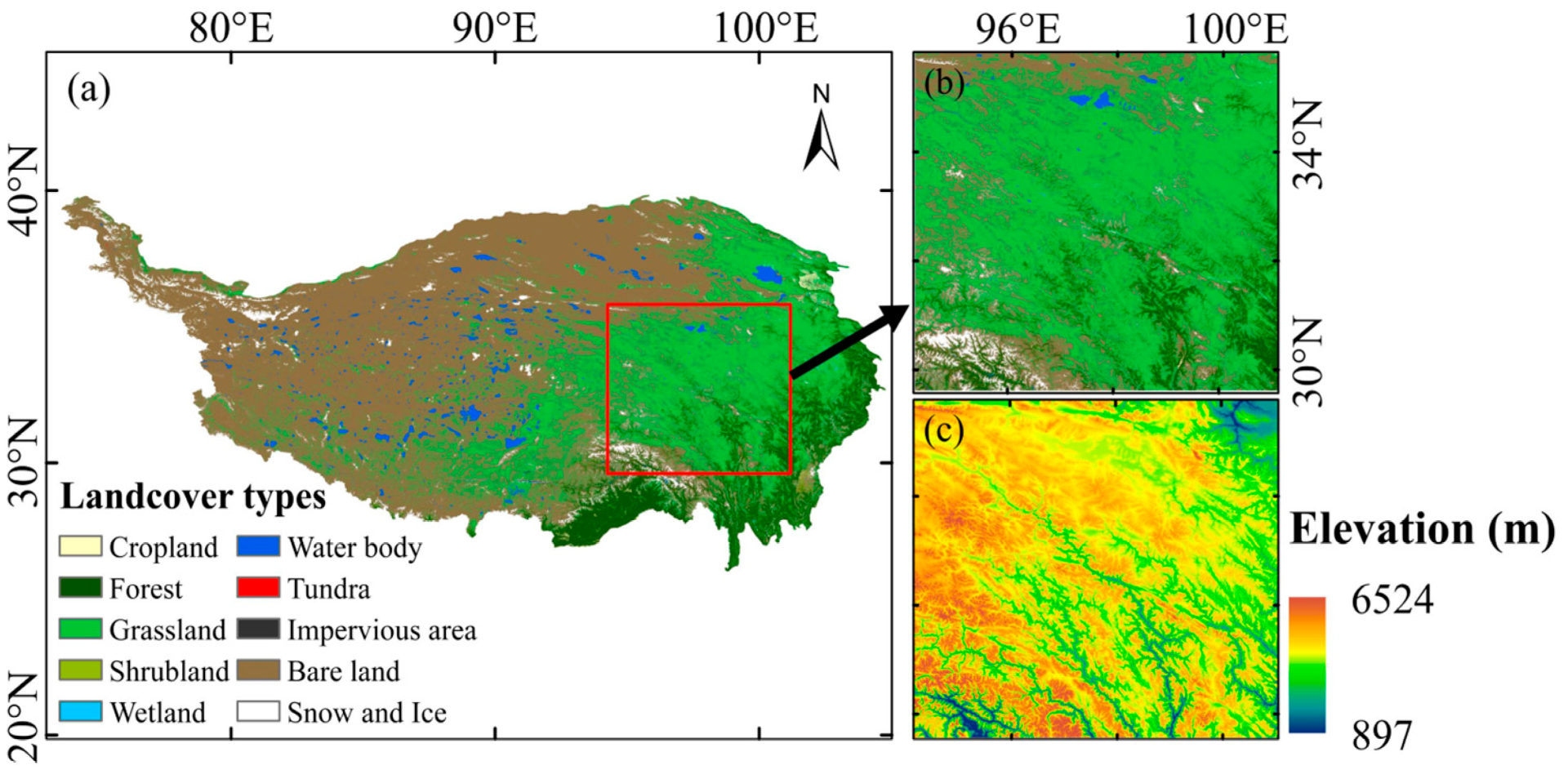
2.1. Study Area

The study area is on the east of the Tibetan Plateau (29°35′30″N–35°48′06″N, 94°08′08″E–101°03′36″E, Figure 1), covering a large area of alpine grasslands at an average elevation of 4000 m. Our study focuses on alpine grasslands, which are dominated by alpine meadows and alpine steppe [41]. The study area is typical of alpine meadows, which normally grow from May to September. The mean temperature ranges from near 0 °C to above 20 °C, and precipitation ranges from 100 mm to over 1000 mm along a south–north gradient [4]. Seasonal snow covers the study area from October to May, which may contaminate the satellite signals and introduce bias in SOS detection.

2.2. Datasets

2.2.1. Satellite Reflectance Data

The MODIS MCD43A4 Nadir Bidirectional Reflectance Distribution Function (BRDF) Adjusted Reflectance (NBAR) product with a 500 m resolution was used in this study to remove the viewing angle effects from directional reflectivity [42]. A total of 366 images from 1 January 2020 to 31 December 2020 were freely downloaded from the NASA Land Processes Distributed Active Archive Center (LP DAAC, http://lpdaac.usgs.gov (accessed on 10 July 2021)), which were processed to UTM/WGS-84 projection and 500 m resolution. Based on repeated manual tests, missing values of 50 consecutive days would introduce significant errors in reconstructing the VI trajectory. To eliminate errors caused by missing values in the daily NBAR products, pixels with more than 50 consecutive days of missing data were flagged as poor-quality pixels and excluded from subsequent analysis, which accounted for only 3.34% of the study area. Reflectance in the red, green, near-infrared (NIR), and shortwave infrared (SWIR) bands was used to calculate the different VIs and to further determine the SOS dates.

2.2.2. Snow Cover Data

The MODIS snow cover data MOD10A2, with a 500 m spatial resolution and 8-day intervals, was used to derive snow phenology parameters in our study. This snow cover product has higher spatial and temporal resolutions [43]. Previous studies have verified that MOD10A2 is effective in reducing the effect of cloud contamination in most cases and has higher classification accuracy than another MODIS snow product (MOD10A1) [37,44]. A total of 46 images from 1 January 2020 to 31 December 2020 were freely downloaded from the National Snow and Ice Data Center (NSIDC, http://nsidc.org (accessed on 17 December 2021)). All images were processed to UTM/WGS-84 projection and 500 m resolution. Pixels coded as ‘200′ were extracted as snow pixels according to the product’s user guide [43].

2.2.3. Land Cover Type and DEM

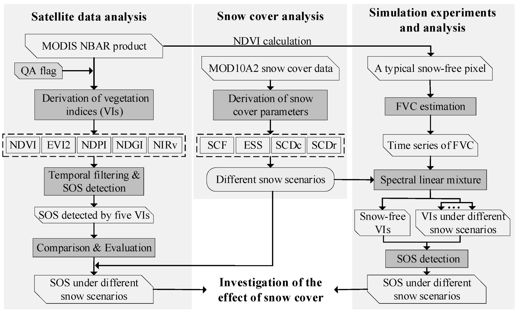
A subset of the global land cover product from Tsinghua University at 10 m resolution in 2017 (available at http://data.ess.tsinghua.edu.cn (accessed on 15 July 2021)) was used to define our study area for its high spatial resolution and high overall accuracy [45], as shown in Figure 1. The SRTM digital elevation model (DEM) data at 90 m resolution were used to characterize the variations in snow phenology and vegetation phenology. The DEM data were freely downloaded from the Geospatial Data Cloud (http://www.gscloud.cn (accessed on 15 July 2021)) and processed to UTM/WGS-84 projection and 500 m resolution, as shown in Figure 1c.

3. Methods

3.1. Derivation of Vegetation Indices

Five VIs were selected and derived from MODIS daily NBAR data for phenology detection, including NDVI, EVI2, NDPI, NDGI, and NIRv. Their definitions and corresponding references are given in

Table 1. Derivation of vegetation indices used in the study.

Index Acronym	Formula	Reference
NDVI	$\mathrm{NDVI}=\frac{R_{\mathrm{NIR}}-R_{\mathrm{Red}}}{R_{\mathrm{NIR}}+R_{\mathrm{Red}}}$	[13]
EVI2	$\mathrm{EVI}2=2.5\frac{R_{\mathrm{NIR}}-R_{\mathrm{Red}}}{R_{\mathrm{NIR}}+2.4R_{\mathrm{Red}}+1}$	[17]
NDPI	$\mathrm{NDP}{I}_{\mathrm{MODIS}}=\frac{R_{\mathrm{NIR}}-[0.74\times R_{\mathrm{Red}}+0.26\times R_{\mathrm{SWIR}}]}{R_{\mathrm{NIR}}+[0.74\times R_{\mathrm{Red}}+0.26\times R_{\mathrm{SWIR}}]}$	[31]
NDGI	$\mathrm{NDG}{I}_{\mathrm{MODIS}}=\frac{0.65\times R_{\mathrm{Green}}+0.35\times R_{\mathrm{NIR}}-R_{\mathrm{Red}}}{0.65\times R_{\mathrm{Green}}+0.35\times R_{\mathrm{NIR}}+R_{\mathrm{Red}}}$	[21]
NIRv	$\mathrm{NIRv}=\mathrm{NDVI}\times R_{\mathrm{NIR}}$	[33]

Note: R_Green, R_Red, R_NIR, and R_SWIR are the surface reflectance values in the green, red, NIR, and SWIR bands, respectively.

.

Among the five VIs, NDVI is the most commonly used VI for monitoring land surface phenology. EVI2 was developed from the enhanced vegetation index (EVI) [46] to adapt to satellite sensors without a blue band [17], while both EVI and EVI2 were designed to overcome the saturation problem and sensitivity to the soil background with NDVI. The NDPI and NDGI and NIRv were recently developed and are rather new. Both NDPI and NDGI were proposed to maximize the contrast between vegetation and soil/snow [21]. The NDPI assumes that the reflectance of soil and snow increases or decreases monotonically from red to SWIR wavelengths. In contrast, the reflectance of vegetation is high in the NIR band and low in both the red and SWIR bands [40]. The NDPI is thus designed by replacing the red band in NDVI with a weighted sum of the red and SWIR bands. As a result, the NDPI is close to zero for soil and snow but high for vegetation [31,40]. NDGI is a semi-analytical snow-free VI based on a linear mixture model. It connects a straight line between the reflectance of the green and NIR bands, and the difference between this line and the reflectance of the red band is defined as the NDGI [21]. NDGI is positive for vegetation but is close to zero for snow, soil, and dry grass. NIRv has been proposed as a proxy for SIF, a very effective indicator of vegetation photosynthesis [47], and has been successfully used in phenology detection [33]. The comparison of these five typical VIs would provide a useful reference for the performance of both structural-based and physiological-based VIs, as well as the traditional VIs and snow-free VIs.

3.2. Spring Phenology Detection and Evaluation

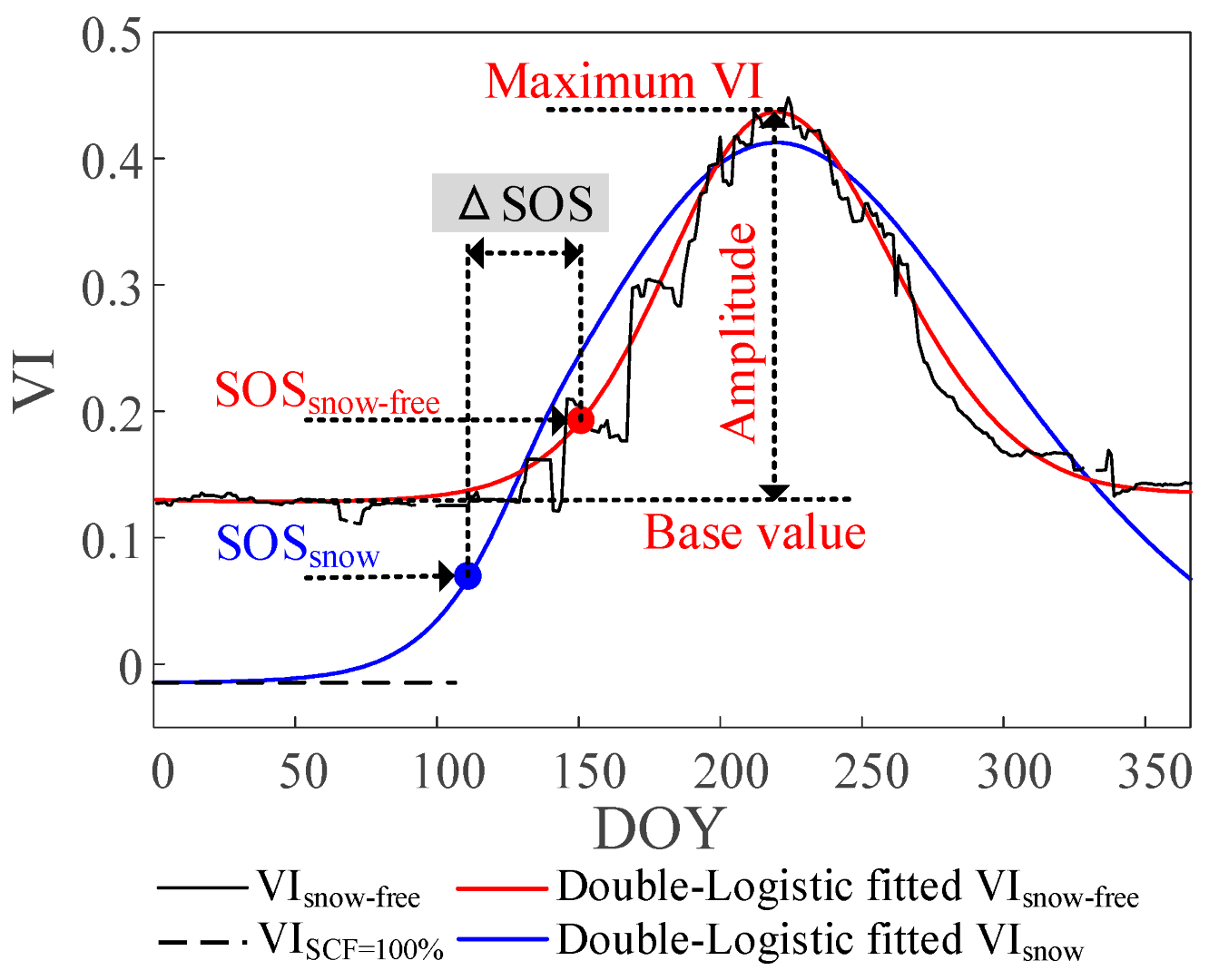
3.2.1. Detection of SOS Dates

Vegetation growth in the alpine grasslands on the Tibetan Plateau has a distinct seasonal cycle, and the SOS can be detected from the time series of five different VIs. We first removed the poor-quality/filled values from the original MODIS datasets and then used a double-logistic fitting method to smooth the noisy time series of VIs in the TIMESAT program [48], since it is more robust in extracting phenological parameters [49,50,51,52]. We applied two upper-envelope iterations with an adaptation strength of 2 to reduce the bias of atmospheric effects in the smoothing process [20]. Then, the simple and intuitive dynamic threshold method [53,54] was used to detect the SOS (Figure 2) for its simplicity and robustness [55], and a 20% amplitude was used to determine the SOS, which was consistent with previous studies [20,55,56]. Figure 2 illustrates how the dynamic threshold method detects the SOS under snow and snow-free conditions. The SOS date was detected as the point in time when the VI increased to 20% of the amplitude plus the base value.

3.2.2. Evaluation of SOS Dates

The SOS detected from the five VIs were compared pixel-by-pixel via scatterplots on each pair of image combinations. Three indicators, the correlation coefficient (R), the mean absolute error (MAE), and the root mean square error (RMSE), were calculated to evaluate the consistency between the SOS detected from different VIs. Then, considering the influence of elevation on the SOS, the study area was divided into four elevation zones, including < 3500 m, 3500–4000 m, 4000–4500 m, and ≥ 4500 m. The changes in the detected SOS dates with varying elevations were analyzed through zonal statistics. The effect of snow on the detected SOS was further analyzed in each elevation zone.

3.3. Effect of Snow Cover on Detecting SOS from VIs

3.3.1. Snow Cover Analysis

Four parameters were used to describe the coverage and phenology of snow, including SCF, SCDc, SCDr, and ESS. The SCF is defined as the snow cover fraction at each location. The SCDc and SCDr are complementary parameters used to describe snow cover duration. The SCDc denotes the maximum number of consecutive days with snow cover and is more specific, while SCDr is defined as the ratio of days with snow to total days and is more general. The SCDc is more ready-to-use in simulating different snow scenarios if we only consider the longest snow duration, while the SCDr is difficult to simulate, as the spring snow cover might include several periods of snow duration. Thus, SCDc was used in both simulations and satellite data analysis, and SCDr was only used in satellite data analysis. The ESS is defined as the ending date of snow, i.e., the last day with snow cover. Since our focus is spring phenology, the SCDc, SCDr, and ESS were calculated for the period from the day of year (DOY) 001 to 208. The four parameters were calculated from the MOD10A2 snow cover data to reveal the spatial and temporal characteristics of snow in the study area. Furthermore, they were also used in simulation experiments to generate different snow scenarios.

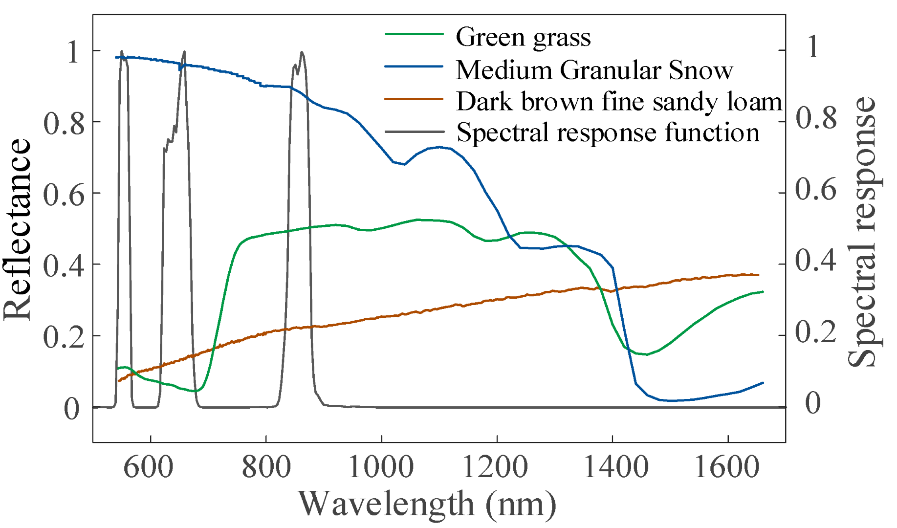
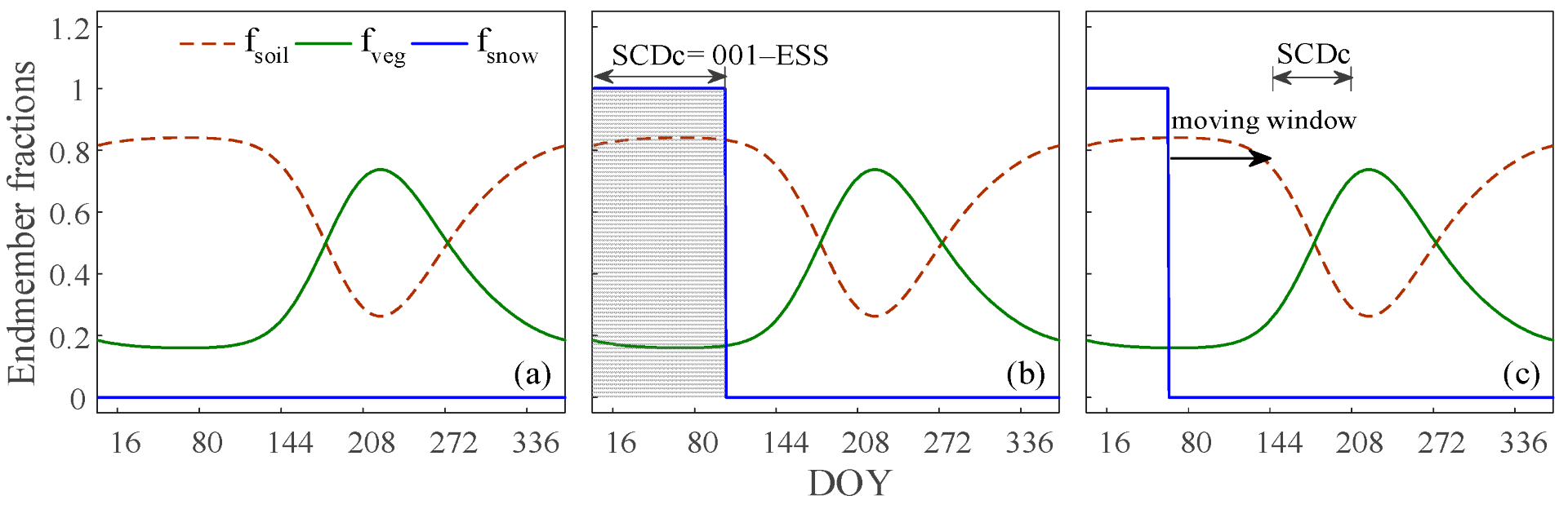
3.3.2. Tests with Simulated Data

Since it is very difficult to find appropriate snow-free vegetation pixels as a reference, we designed simulation experiments to evaluate the effect of snow on SOS detection. A linear spectral mixture model was used to simulate the pixel reflectance with different SCF values. For simplicity, it is assumed that each pixel is composed of soil and vegetation; the snow layer is covered above and only absorbs and reflects the incident light, i.e., the transmittance of the snow layer equals 0. Assuming that the vegetation and soil components are both homogeneous, which is reasonable for alpine grasslands, the presence of snow will not affect the areal compositions of soil and vegetation. As a result, the spectral reflectance of a snow-covered pixel can be computed as:

$$R_{\mathrm{mixed}}=(1-f_{\mathrm{snow}})\left[f_{\mathrm{veg}}\cdot R_{\mathrm{veg}}+(1-f_{\mathrm{veg}})R_{\mathrm{soil}})\right]+f_{\mathrm{snow}}\cdot R_{\mathrm{snow}}$$

(1)

where R_mixed denotes the simulated mixed pixel reflectance; f_veg, f_soil, and f_snow are the coverage fractions of vegetation, soil, and snow, respectively; and R_veg, R_soil, and R_snow are the corresponding endmember reflectances.

To simulate the satellite-derived band reflectance, the spectral reflectance ρ(λ) was convolved with the spectral response function (SRF) of the MODIS sensor S(λ) as follows:

$$R={\displaystyle {\int }_{{\lambda }_1}^{{\lambda }_2}\rho }(\lambda )S(\lambda )\mathrm{d}\lambda$$

(2)

where λ1 and λ2 are the minimum and maximum wavelengths of each band, respectively. The ρ(λ) for snow, soil, and vegetation were selected from the Johns Hopkins University Spectral Library [57], corresponding to medium granular snow, dark brown fine sandy loam, and green grass, respectively, as in Figure 3.

Through Equations (1) and (2), the band reflectance and further VIs of a pixel can be computed using the endmember reflectance with varying FVC and SCF values. To investigate the effect of snow cover on SOS detection, simulation experiments were designed in the following two aspects.

First, we investigated the effect of snow cover on five VIs. We computed the VI values when FVC was varied from 0 to 1 for five cases of SCF = 0%, 25%, 50%, 75%, and 100%. The effect of snow cover on VI values can be described by the difference in VI values under specific snow scenarios and snow-free conditions (i.e., SCF = 0%), expressed as ΔVI = VI_{SCF > 0} − VI_{SCF = 0}. As the values of ΔVI vary with SCF and FVC, we further define a quantitative indicator, the maximum impact of snow (MIS), to represent the maximum effect of snow on VI for a specific FVC, expressed as:

$$\mathrm{MIS} =\frac{\left|{\mathrm{VI}}_{\mathrm{SCF} = 100\%}-{\mathrm{VI}}_{\mathrm{SCF} = 0\%}\right|}{{\mathrm{VI}}_{\max }-{\mathrm{VI}}_{\min }}$$

(3)

where VI_{SCF = 100%} and VI_{SCF = 0%} correspond to VI values when SCF = 100% and SCF = 0% for a given FVC, respectively; VI_max and VI_min are the maximum and minimum VI values, respectively. The denominator is the range of VI values and is used to eliminate the effect of different value ranges of VIs. Both VI and MIS vary with FVC. The numerator represents the absolute difference in VI between SCF = 100% and SCF = 0%, while the MIS represents the maximum percentage change in VI caused by snow relative to the range of VI values. The MIS provides a direct indication of the extent to which a VI is affected by snow and provides a basis to further investigate the effect of snow cover on SOS detection.

Second, to investigate the effect of snow cover on SOS detection, we designed a series of experiments to generate different VI time curves under different snow scenarios. We extracted the NDVI time curve of a typical snow-free vegetation pixel and converted the time series of NDVI to FVC using the dimidiate pixel model [58]. Using the derived time series of FVC, the time series of band reflectance and VI were calculated under different snow scenarios defined by snow parameters, including SCF, SCDc, and ESS. The time curves of five different Vis were then filtered, and the SOS was detected. As shown in Figure 2, given the same growth curve of FVC, the red and blue lines represent the VI trajectories for snow-free and preseason snow conditions, respectively. The preseason snow caused a bias in the detected SOS, expressed as ΔSOS = SOS_snow − SOS_snow-free, which is defined as the effect of snow on SOS detection.

Three sets of experiments were designed, and the corresponding settings of snow scenarios are shown in

Table 2. Experimental settings for the investigation of the effect of snow on spring vegetation phenology detection.

Experiments No.	Snow Scenarios *
I	Snow free with SCF = 0% constantly during the period from DOY 001 to 208.
II	Snow persists from DOY 001 to ESS (DOY 104, 136, and 168) with constant SCF.
III	Snow persists from DOY t to ESS with constant SCF, where t is iterated from DOY 001 at 16-day interval; ESS = t + SCDc − 1 ≤ 208; and SCDc = 32, 64, and 96 days.

* In experiments II and III, four cases with SCF = 25%, 50%, 75%, and 100% were considered.

. In all experiments, as we were only concerned with the SOS, only the snow season from DOY 001 to DOY 208 was considered. Experiment I corresponded to a completely snow-free case with SCF = 0% during the period, which served as the baseline to assess the effect of snow cover on SOS detection (Figure 4a). Experiments II and III were snow cover conditions, where four cases of SCF = 25%, 50%, 75%, and 100% were considered, and in all cases, the SCF remained constant during the snow season. Experiment II referred to the cases of snow persisting from DOY 001 to ESS. Three cases of ESS at DOY 104, 136, and 168 were considered, which were the mean ESS plus or minus its standard deviation analyzed from snow cover data, as shown in Figure 4b. In experiment III, three cases of SCDc = 32, 64, and 96 days were considered. As the SCDc could be in any interval during the snow season, we simulated all cases by iterating the start of the snow season from DOY 001 at 16-day intervals while keeping the ESS no later than DOY 208. For example, a case with SCDc = 64 can generate 10 different time curves of a VI with a snow season ranging from DOY 1–64 to 145–208, as shown in Figure 4c.

3.3.3. Tests with Satellite Data

Since snow is prevalent, a direct comparison of VI in snow-covered and snow-free pixels is difficult. Based on the simulation results, the effect of snow cover on SOS detection was analyzed from satellite data in two aspects. First, the statistical distribution of the minimum and maximum values of VI over time for each SCDr interval in each elevation zone was analyzed. This analysis could help reveal the difference in VI values between different SCDr intervals in the same elevation zone. Second, the statistical distribution of the SOS detected from real satellite data for different SCDc and ESS scenarios was analyzed, which could help reveal the variations in the detected SOS under different SCDc and ESS cases.

The flowchart of this study is shown in Figure 5.

4. Results

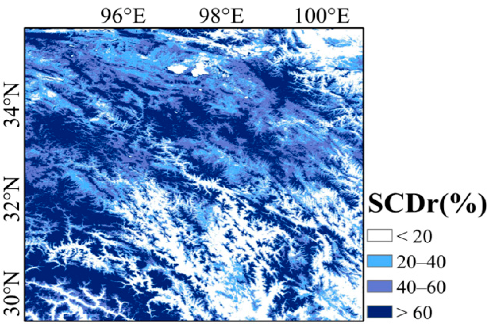
4.1. Snow Cover Analysis

The snow cover analysis from MOD10A2 data in Figure 6 shows that a large portion of the study area was covered by snow, while the SCDr varied across the area. Statistically, the SCDr in 52.27% of the study area was higher than 40%, and the SCDr was lower than 20% only in 21.25% of the study area.

Statistically, approximately 77% of the study area has an elevation ≥ 4000 m, while only approximately 6% of the area has an elevation < 3500 m. Figure 7 shows the statistical distributions of ESS, SCDr, and SCDc in each elevation zone. In all four elevation zones, the ESS values were concentrated on DOY 136. The increase in elevation led to the increase in ESS. When the elevation increased to ≥4000 m, a significant subpeak in the ESS appeared on DOY 160. Both SCDr and SCDc increased with increasing elevation. The peak values of SCDr were 0%, 8%, 36%, and 64%, while the peak values of SCDc were 8, 8, 16, and 88 days, respectively, for all four elevation zones from elevations <3500 m to ≥4500 m.

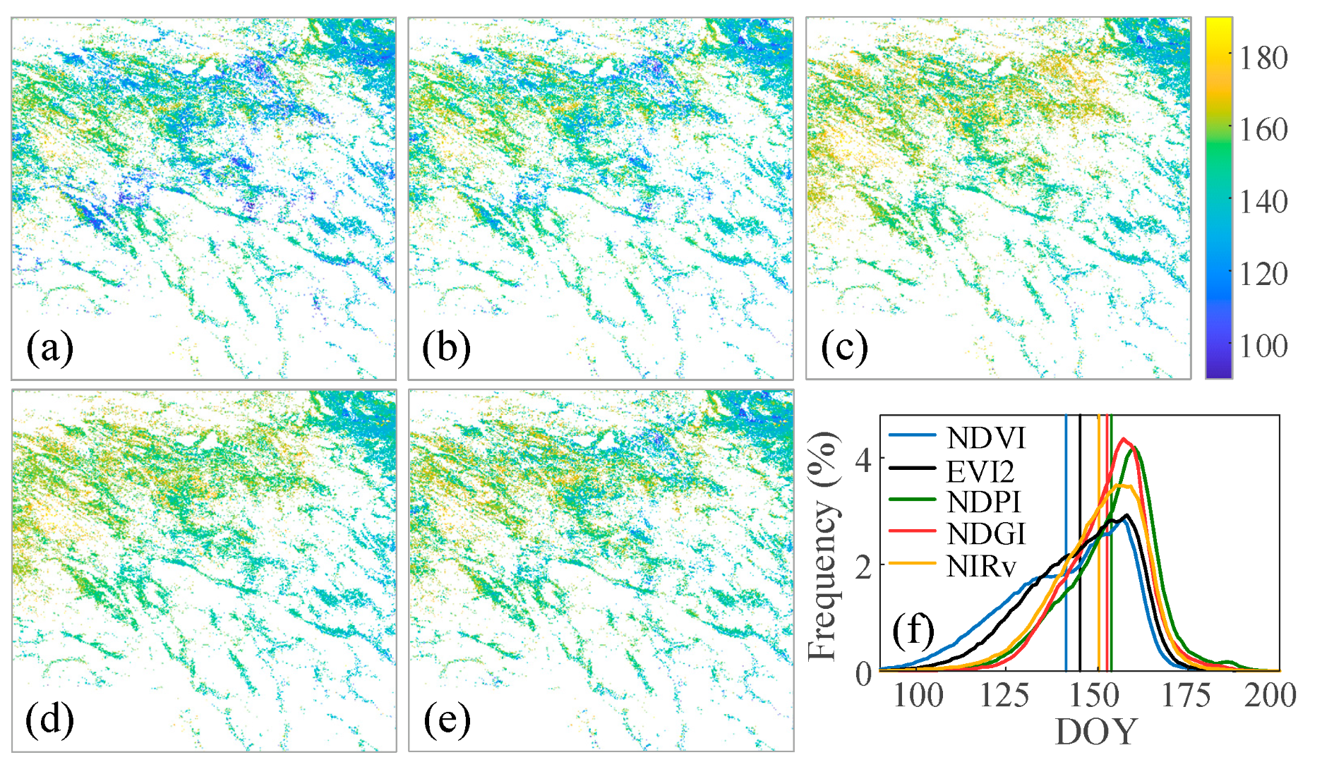
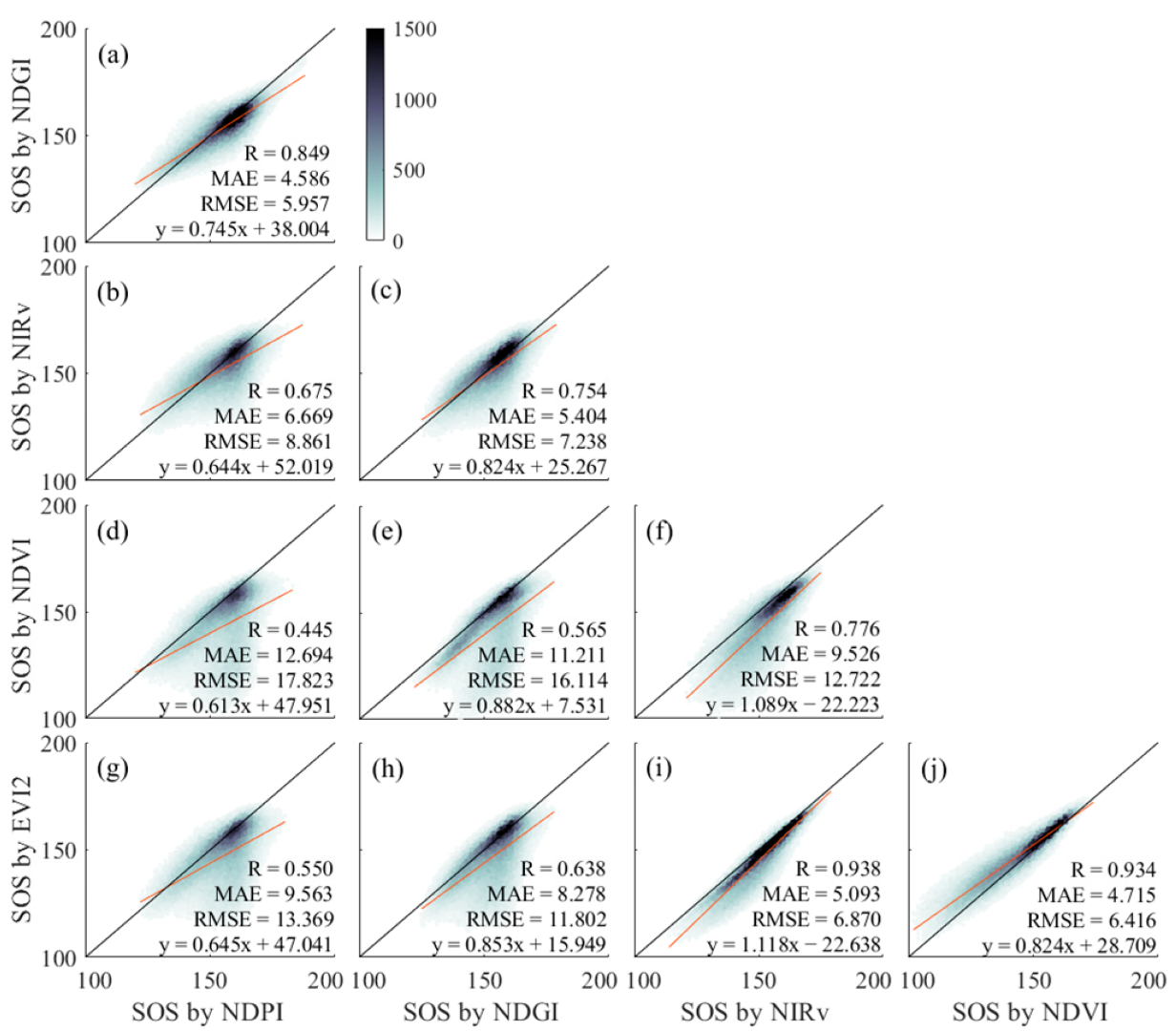
4.2. Spring Phenology Derived from Different VIs

Figure 8 shows the SOS detected from five different VIs. Nongrassland pixels (e.g., water bodies, forests, etc.) and the pixels whose SOSs were poorly detected were flagged as no data. SOS trends derived from different VIs were generally spatially consistent with the elevation variations. The SOS dates in the eastern part of the study area were earlier than those in the western parts. As shown in Figure 8, the SOS dates detected by NDVI were very similar to the SOS dates detected by EVI2, while those from NDPI and NDGI were highly consistent and those detected by NIRv were in between. The histograms revealed that the SOS dates detected by the five VIs were generally similar in terms of the value ranges and peak values. The detected SOS dates ranged from 105 to 175, while the average SOS dates derived from the five VIs followed the order of NDPI (DOY 154) > NDGI (DOY 152) > NIRV (DOY 150) > EVI2 (DOY 145) > NDVI (DOY 141), which was very consistent with previous studies in this study area [38,55,59]. This indicates that the SOS dates detected by the five VIs were generally consistent and reliable.

Scatterplots in Figure 9 compare the SOS dates detected from different VIs on a pixel-by-pixel basis. According to the consistency between the detected SOS, the five different VIs were aggregated into two groups. One group included NDGI and NDPI (R = 0.849 and RMSE = 5.957), and the other group included EVI2, NDVI, and NIRv. The SOS dates detected by EVI2 were highly correlated with those detected by NDVI (R = 0.934 and RMSE = 6.416) and NIRv (R = 0.938 and RMSE = 6.870), while the SOS detected by NDVI and NIRv had lower correlations (R = 0.776 and RMSE = 12.722). The SOS detected by the VIs from different groups showed large discrepancies. For example, the SOS dates from NDVI and NDPI were poorly correlated (R = 0.445) and had a large bias (RMSE = 17.823). In addition to the differences in VI calculations, this different performance may also be attributed to the different effects of snow cover on different VIs.

4.3. Simulation Results

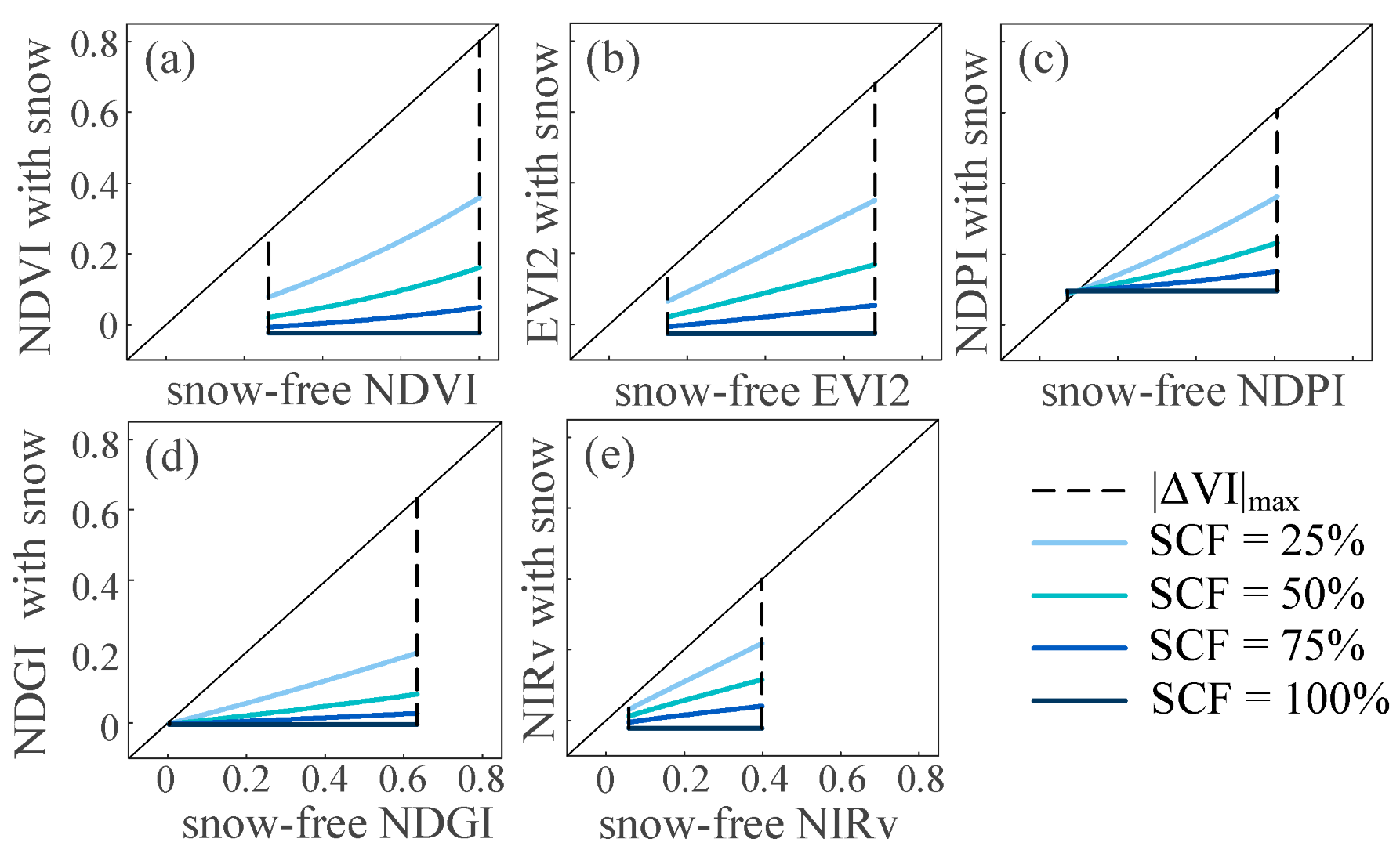
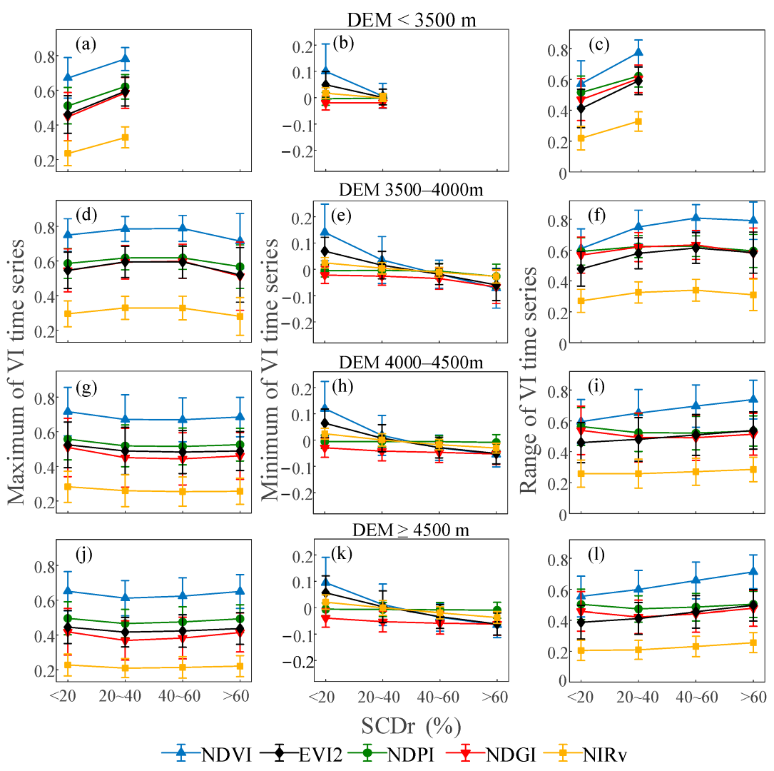
4.3.1. Effect of Snow Cover on VI

Figure 10 compares the changes in the five VIs under different SCF conditions as the FVC increases from 0 to 1. For all indices, the values of the five VIs generally decreased with increasing SCF. In the presence of snow cover, the larger the FVC was, the greater the decrease in the VI value. The deviation of the data points from the 1:1 line showed the effect of snow cover on VI values. The dashed line in each subplot of Figure 10 indicates the difference in VI values between SCF = 0% and SCF = 100%, denoted as |ΔVI|_max. MIS values were further calculated for FVC = 0 and FVC = 1 to show the maximum possible influence of snow on VI values using Equation (3). Thus, the sensitivity of the five VIs to snow cover is NDPI (MIS range 0.0466–0.9534) < NDGI (MIS range 0.0122–1.0122) < NIRv (MIS range 0.2335–1.2335) < EVI2 (MIS range 0.3320–1.3320) < NDVI (MIS range 0.5280–1.5280).

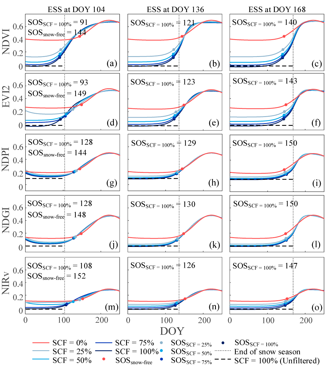
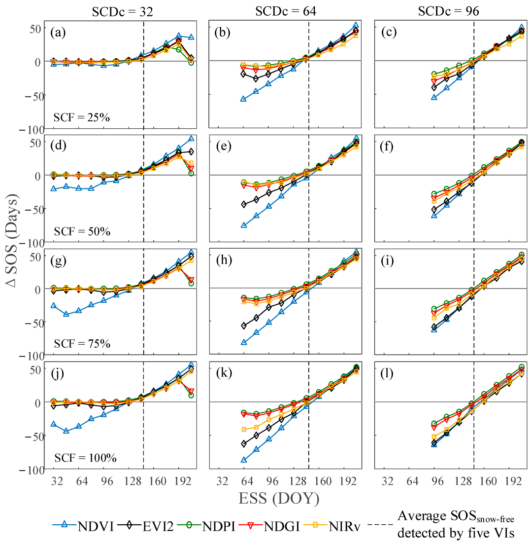
4.3.2. Effect of Snow Cover on SOS Detection

Figure 11 shows the temporally filtered time curves of the five VIs and the detected SOS dates in simulation experiments I and II. Under snow-free conditions, the SOS detected by the different VIs ranged from DOY 144 to DOY 152, indicating small differences in snow-free SOS detected by the different VIs. Under snow conditions, the SOS dates detected by NDVI and EVI2 were earlier, while those detected by NDGI and NDPI were later, and those detected by NIRv were in between, as shown in all subplots of Figure 11.

Considering the differences in the SOS between SCF = 0 and SCF > 0 in Figure 11, the effect of snow on the detected SOS generally follows the order of NDPI/NDGI < NIRv < EVI2/NDVI. Generally, the presence of snow significantly reduced the VI values during the pregrowth period and advanced the SOS for all five VIs. For all five VIs, the greatest advances in the SOS were found for the earliest snow season (i.e., for ESS at DOY 104), which ranged from 16 to 56 days. As the ESS increased from DOY 104 to 168, the advances in the detected SOS decreased rapidly. For the ESS at DOY 168, the SOS estimated by NDVI, EVI2, and NIRv was only 4–6 days earlier than the snow-free SOS, while those estimated by NDPI and NDGI were 6 and 2 days later than the snow-free SOS, respectively. This indicates that the ending date of persisting snow is very important. When persisting snow ends earlier than the snow-free SOS, the presence of snow reduces the minimum VI value during the pregrowth period but does not affect the maximum VI value during the peak growth period, which would increase the gradient of the time curve of VI significantly and cause the SOS to be detected earlier. As analyzed in Section 4.3.1, the snow-induced decrease in the VI value is very small at small VI values and is relatively larger at large VI values. When the snow season ends later than the snow-free SOS, the decrease in VI values around the SOS is larger than that of the pregrowth period. This may locally smooth the time curve of VI and delay the detected SOS compared to the case of an early snow season.

To further investigate the mechanism of how snow affects SOS detection, simulation experiment III was implemented to analyze the ΔSOS under different snow scenarios defined by SCDc, ESS, and SCF, and the results are shown in Figure 12. It clearly shows that ΔSOS changes with varying SCDc, ESS, and SCF values. Using the absolute values of ΔSOS as a standard, the effect of snow on SOS detection followed the order of NDPI/NDGI < NIRv < EVI2 < NDVI, which is consistent with the effect of snow on VI values analyzed in Section 4.3.1. Both SCDc and ESS are very important in determining the ΔSOS. In general, the larger the SCDc value was, the larger the absolute value of ΔSOS. This is reasonable because the reduction in VI values during a short snow period (i.e., small SCDc) can be better recovered by time series filtering performed prior to SOS detection. Specifically, for short snow with SCDc = 32, ΔSOS was very close to 0 for all VIs, except NDVI, for which ESS was earlier than the snow-free SOS. For longer snow with SCDc = 64 and 96, ΔSOS increases from negative to positive values as ESS increases. This also indicates that an earlier ESS generally advances the SOS, while an ESS much later than the snow-free SOS delays the SOS, and ΔSOS approaches 0 when ESS approaches the snow-free SOS. These findings were consistent with the results of experiments I and II as analyzed above.

To further investigate the different effects of ESS and SCDc on ΔSOS, we also analyzed the time curves of Vis under different ESS scenarios based on simulation experiment III. The medium SCDc = 64 was used. As the ΔSOS was close to 0 around the ESS at DOY 144, the ESS was varied as DOY 144 minus or plus three 16-day intervals, corresponding to three cases of ESS at DOY 96, 144, and 192. Figure 13 shows the temporally filtered time curves of VIs and the detected SOS. It clearly shows that the snow season ending much earlier than the snow-free SOS (ESS at DOY 96) advanced the SOS by up to 56 days, while the snow season ending much later than the snow-free SOS (ESS at DOY 192) delayed the SOS by up to 38 days. When the ESS approached the snow-free SOS (ESS at DOY 144), the changes in SOS caused by snow were very small. Therefore, the effect of snow cover on SOS detection depends on snow parameters, specifically SCDc, ESS, and the snow-free SOS. Because the presence of snow increases the local gradient of the VI growth curve and causes SOS to be detected, ESS and snow-free SOS determine where and to what extent the gradient of the VI growth curve increases.

4.4. Effect of Snow Cover on Spring Phenology Detection from Satellite Data

4.4.1. Effect of Snow Cover on VI

Figure 14 shows the statistical distributions of the maximum, minimum, and range of the time series of VIs for different SCDr intervals within the same elevation zone. To ensure a sufficient number of pixels for statistics, the SCDr intervals with too few pixels were excluded from the subsequent analysis, including the intervals of SCDr = 40–60% and SCDr > 60% in the zone of DEM < 3500 m. Generally, the decrease in minimum VI values with increasing SCDr was more significant than the decrease in maximum VI values. This is because snow always melts before the peak growth season and does not affect the maximum VI over time. Consequently, the range of VI values increased with the increasing SCDr for all five Vis. These findings were consistent with the simulation results. However, the reduction in VI values with increasing SCDr was not as significant as in the simulation results. This is probably because there were few snow-free pixels, and the minimum VI in the interval SCDr < 20% was affected by snow. Based on the decrease in the minimum VI value with increasing SCDr, the effect of snow on the VI value follows the order of NDPI/NDGI < NIRv < EVI2 < NDVI, which was consistent with the findings from the simulation experiments described in Section 4.3.1.

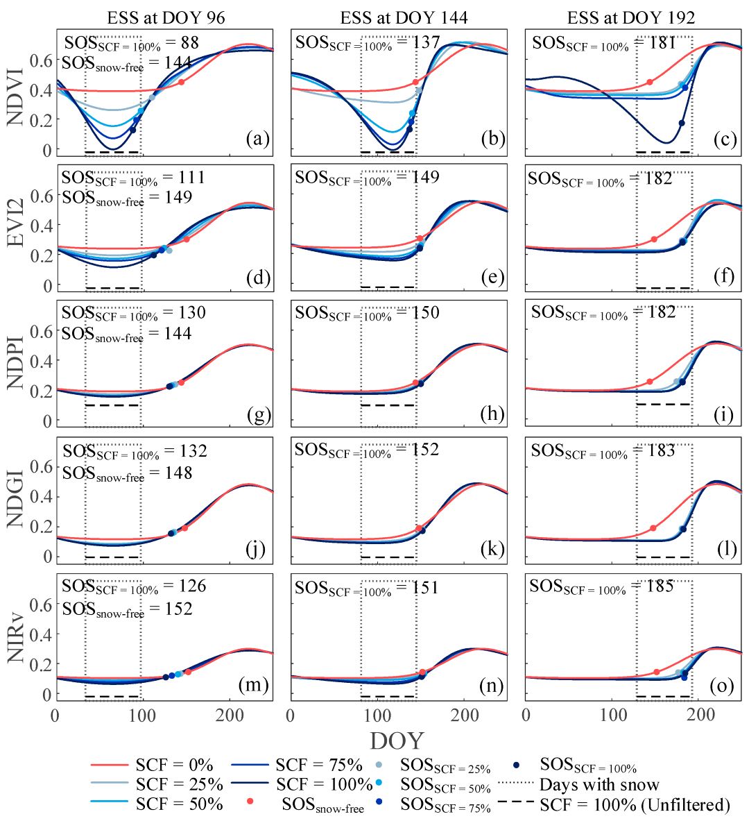
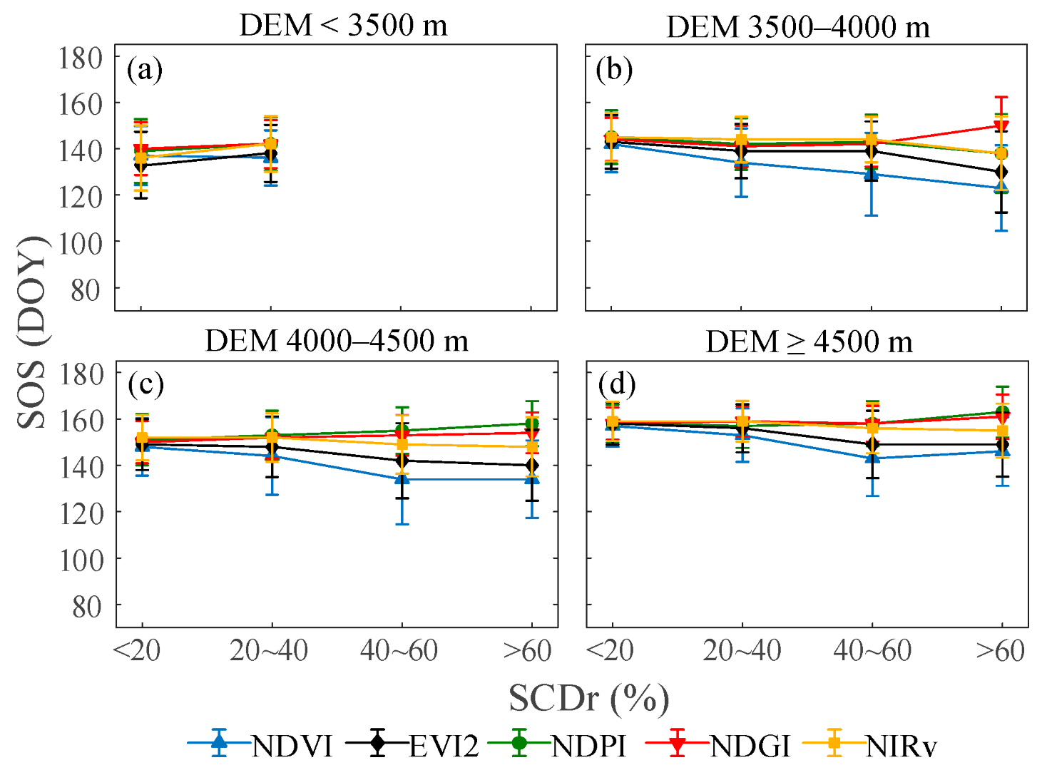
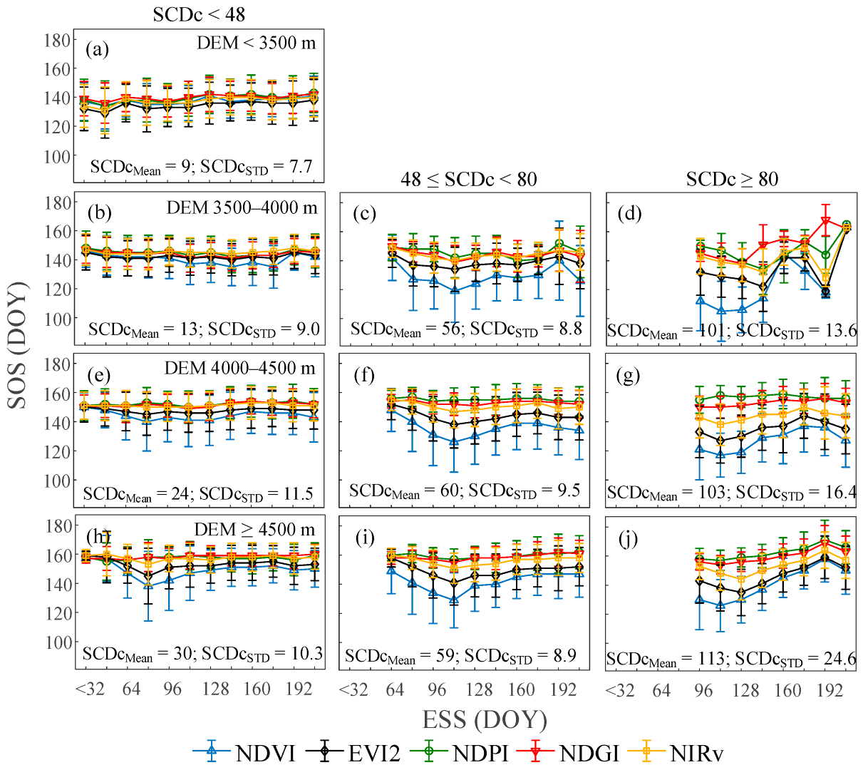
4.4.2. Effect of Snow Cover on SOS Detection

Figure 15 compares the statistical distribution of SOS detected from the five VIs at different SCDr and elevation zones. At the same SCDr, an increase in elevation caused a delay in the SOS for all five VIs. For less snowy areas with SCDr < 20%, an increase in elevation from < 3500 m to ≥ 4500 m caused a delay of approximately 19–25 days. Within the same elevation zone, the increase in SCDr caused different effects on the SOS detected by different VIs. At elevations ≥ 4500 m, an increase in SCDr from < 20% to > 60% delayed the SOS by 3 and 5 days for NDGI and NDPI, respectively, but advanced the SOS by 11, 9, and 4 days for NDVI, EVI2, and NIRv, respectively. Generally, the SOS detected by NDGI, NDPI, and NIRv was less affected by snow, while the SOS detected by NDVI and EVI2 was more affected by snow.

Based on the simulation results, the effect of snow on SOS detection depends on SCDc, ESS, and snow-free SOS. Figure 16 shows the statistical distribution of the SOS for different SCDc and ESS cases in each elevation zone using real satellite data. To ensure sufficient pixels for the statistical analysis, we considered three SCDc cases, including SCDc < 48, 48 ≤ SCDc < 80, and SCDc ≥ 80, and divided the ESS values into 12 cases with 16-day intervals from DOY 32 to 208. In the zone with DEM < 3500 m, the intervals of 48 ≤ SCDc < 80 and SCDc > 80 had a maximum of two pixels and were excluded from the statistical analysis.

As shown in Figure 16, the effect of snow on the detected SOS followed the order of NDPI/NDGI < NIRv < EVI2 < NDVI. Generally, the larger the SCDc was, the larger the effect of snow cover on the detected SOS. For short snow (i.e., SCDc < 48), the fluctuation in the SOS with varying ESS was the smallest for all five Vis, indicating a negligible effect of snow. Using the SOS detected for short snow (i.e., SCDc < 48) as a benchmark, the SOS detected under medium snow (i.e., 48 ≤ SCDc < 80) was generally advanced for NDVI and EVI2 and was slightly delayed for NDPI, NDGI, and NIRv for ESS later than DOY 144. For long snow (i.e., SCDc ≥ 80), the detected SOS dates were advanced for ESS earlier than DOY 160 and delayed for ESS later than DOY 160. For short and medium snows, the effect of snow on SOS detection was generally small for NDPI, NDGI, and NIRv. Generally, an earlier ESS results in earlier estimates of the SOS, while a later ESS results in later estimates of the SOS. These findings were highly consistent with the simulation results and verified the validity of the simulation experiments.

5. Discussion

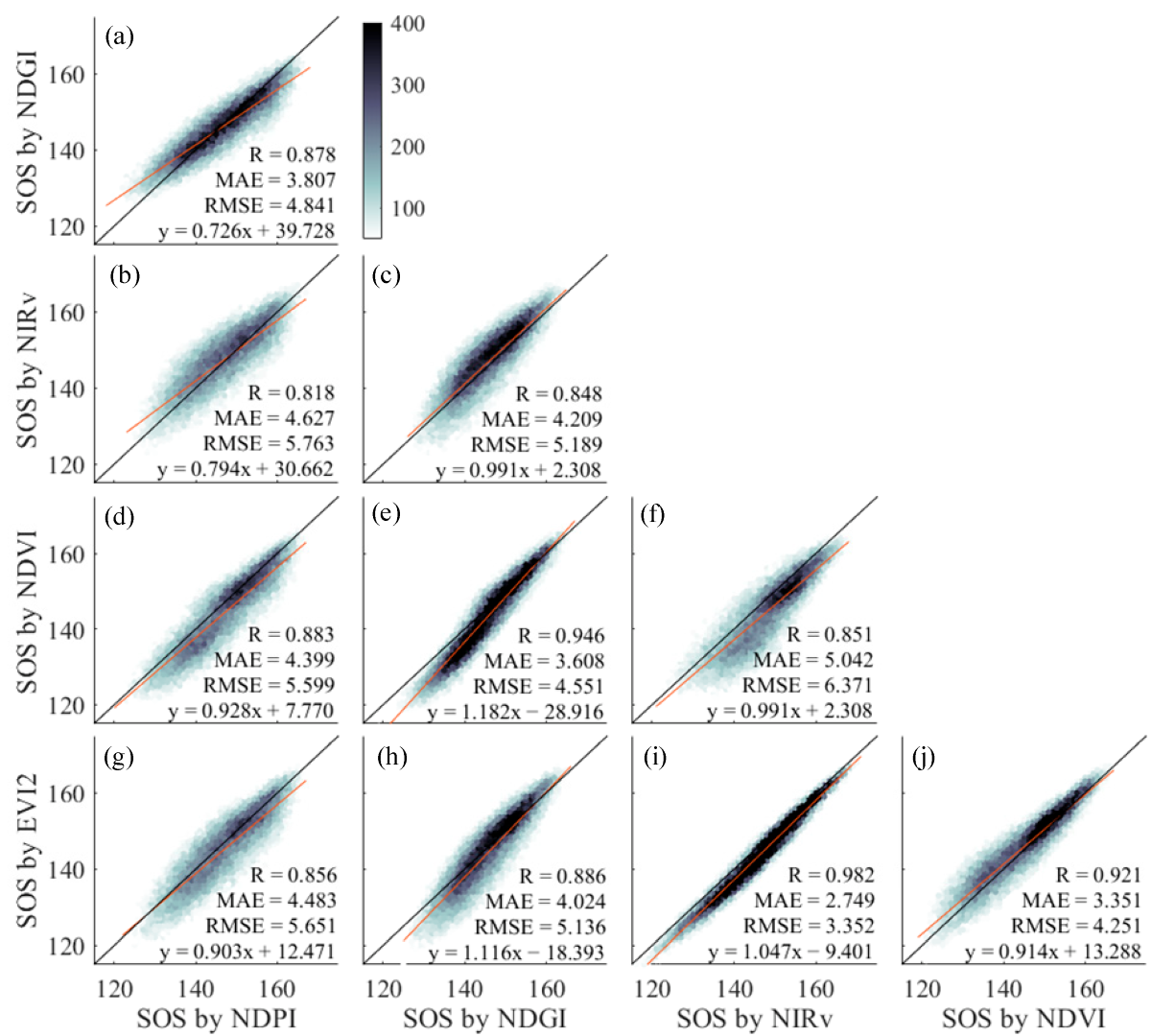
5.1. Validity of the SOS Dates Detected by Different VIs

The SOS dates detected by the five different VIs all captured the spatial pattern of the SOS, which occurred earlier in the eastern areas and later in the western areas (Figure 8). The SOS dates detected by five different VIs also have very similar data distributions, ranging from 105 to 175 with peak values of approximately 157. Both the spatial details and data values were highly consistent with each other and with previous studies [38,55,59], verifying the validity of the detected SOS dates.

Statistical analysis in Figure 15 revealed that both the mean and standard deviation values of the SOS detected in less snowy areas (e.g., SCDr < 20%) by different VIs were very close to each other. However, for more snowy areas, such as for SCDr > 40%, discrepancies occurred in the SOS detected by different VIs. The SOS derived from NDVI and EVI2 were earlier, while those from NDPI and NDGI were later and those from NIRv were in between. These discrepancies could be attributed to the different sensitivities of various VIs to preseason snow cover.

For the entire study area, the SOS dates detected by different VIs have different correlations with each other, such as the results of NDGI/NDPI, which have relatively low correlations with those of NDVI/EVI2/NIRv. However, for less snowy areas, very high correlations were found for the results of all five VIs. Figure 17 compares the different SOS results for the areas with SCDr < 20%. The R values between the different SOS results ranged from 0.818 to 0.982, indicating a very high consistency of the SOS detected by different VIs.

Although previous studies confirmed the accuracy of satellite-derived SOS dates under snow-free conditions [20,21,31,40], a direct comparison with field data was lacking in this study due to the unavailability of in situ SOS measurements. However, we referred to previous studies [20,38,55,59,60] and found a high consistency of our results with the previous in situ measurements and satellite-derived SOS dates in terms of value ranges and spatial distribution. Moreover, a high consistency of the SOS results detected by different VIs was confirmed for less snowy conditions, which was also consistent with previous findings [19,20]. Since the satellite-derived SOS dates represent the macroscale spring phenology and cannot be simply equated with the in situ measurement [61,62], the absence of a direct comparison with in situ measurements does not affect the validity of our results, yet we hope more evidence from in situ measurements to support our findings in the future.

5.2. Influence of Snow Phenology Parameters

Both the simulation experiments and satellite data analysis showed that the presence of snow could significantly reduce the VI values, increase the local gradient of the time curve of VI during pregrowth periods, and cause the SOS to be detected. The bias in the SOS (ΔSOS) caused by snow cover depends on snow phenology parameters, especially the SCDc, ESS, and snow-free SOS.

In general, the SCDc represents the maximum duration of snow cover, corresponding to the length of the reduced values in the VI trajectory, which determines whether the reduced VI values could be recovered from temporal filtering. Thus, the larger the SCDc value was, the larger the absolute value of ΔSOS. Compared to the SCDc, the SCDr only represents overall snow-covered days. A high SCDr does not necessarily imply a high SCDc, while a high SCDc does lead to a high SCDr. Thus, the relationship between the SCDr and ΔSOS was rather indirect and was not discussed in detail.

Whether the ESS is earlier or later than the snow-free SOS determines whether ΔSOS is negative or positive, corresponding to the advancement or delay of the SOS detected under snow conditions. The further the temporal distance of ESS to the snow-free SOS was, the larger the absolute value of ΔSOS. These findings were consistent with previous studies [37,38,63,64]. An earlier ESS results in an earlier estimate of SOS, while a later ESS results in a later estimate of SOS. For example, Wang et al. [38] analyzed the correlation between the duration of snow cover and the SOS on the Qinghai–Tibet Plateau and found that snow cover can advance the SOS in the northeastern, central, and southwestern edges of the Qinghai–Tibet Plateau; however, in some areas, longer snow cover duration delayed the SOS. Xie et al. [64] found that a shortened snow duration advances the SOS, whereas a prolonged snow duration delayed the SOS in their study in the European Alps.

5.3. Performance of Five VIs under Snow Conditions

Our study showed that the effects of snow cover on the five VIs were NDPI < NDGI < NIRv < EVI2 < NDVI. For SOS detection, NDPI and NDGI were rather stable even with winter snow cover, which verified their abilities to minimize the effect of snow cover for alpine grasslands, such as those also found for the American prairie [65]. Our study further revealed the variations in the ΔSOS with snow phenology parameters for NDPI and NDGI. For short and medium snow (i.e., SCDc ≤ 64), preseason snow ending prior to the snow-free SOS caused insignificant biases in the SOS detected by NDPI and NDGI. For long snow (i.e., SCDc ≥ 96) or late snow that ends far later than the snow-free SOS, the biases in the SOS detected by NDPI and NDGI are significant. These findings increase our knowledge about the specific conditions under which the NDPI and NDGI are reliable for SOS detection with snow cover. The traditional NDVI and EVI2 are easily and heavily affected by snow cover. Either an early or a late snow season can cause significant bias in the detected SOS. The physiological-based NIRv could derive SOS dates highly consistent with those detected by NDVI and EVI2 and was less sensitive to snow cover than NDVI and EVI2, indicating its great potential for phenological detection in alpine grasslands. These findings with respect to the performance of different VIs under snow conditions were consistent with the study of Yang et al. [21].

5.4. Limitations and Future Improvements

There are several state-of-the-art methods to smooth the temporal profiles of VIs and extract phenological metrics [11,52,66,67,68]. Only one of them was used in this study. More methods can be used and evaluated in further studies. However, we assumed that the conclusion can hold for other SOS detection method because the affecting mechanism of snow in increasing the local gradient of the growth curve is still valid. A previous study using the derivative-based method for SOS detection achieved similar conclusions that snow cover would advance the SOS, but prolonged snow duration would delay the SOS date [38].

The design of the simulation experiments made a series of simplifications of the actual situation. One major simplification is that light cannot penetrate the snow layer. This assumption is representative of most cases with a thick snow layer but may not apply to thin snow layers. However, thin snow can melt or form into a thick snow layer quickly, which will cause negligible effects on the time curves of the VIs. This assumption is thus reasonable, yet further studies can consider the case of temporary thin snow. The other major simplification is that we only considered the presence or absence of snow cover without considering the snowmelt process. Snowmelt can also last for several days and affect vegetation phenology [39,69]. Although such simplification would cause a sharp increase in the time curve of the VIs at the ESS, temporal smoothing performed prior to the SOS detection can locally smooth the VI temporal curve and remedy the problem. In addition, the simulation experiments showed that a small SCF, such as 25%, can cause a large reduction in the VI value. Although the snowmelt process leads to a gradual decrease in SCF, the largest increase in the VI value is expected to be at the stage when SCF decreases from 25% to 0%, which is a relatively short time interval. Therefore, the presence and immediate melting of snow in our simulation experiments is reasonable, and more complex situations can be considered in future work.

For the debate on whether NDVI-based spring phenology trends are overestimated on the Tibetan Plateau [6,7,30,70], we suggest that snow phenology, particularly ESS, should be given much attention in related studies. Normally, NDPI, NDGI, and NIRv would be less affected by snow cover, and their performance in detecting long-term phenology trends can be further investigated. Based on the findings in this study, we also expect to decouple the effect of snow cover on satellite signals and on vegetation physiological phenology, which will enhance our understanding of vegetation–climate feedbacks.

6. Conclusions

Considering the difficulty in assessing the effect of snow cover on SOS detection, this study investigated the effect of snow cover on both VI and SOS detection by combining simulation experiments and real satellite data, aiming to determine how snow affects the different VIs and the subsequent SOS detection and how different VIs perform in capturing the SOS for alpine grasslands on the Tibetan Plateau. Five VIs, including NDVI, EVI2, NDPI, NDGI, and NIRv, were used for SOS detection, and their performance was compared.

Based on the simulation experiments, we found that the presence of snow, even at a low SCF, can significantly reduce the values of the five VIs and increase the local gradient of the growth curve, allowing the SOS to be detected. Thus, the bias in the detected SOS due to snow cover depends on both snow phenological parameters (i.e., ESS and SCDc) and the snow-free SOS. An earlier ESS results in an earlier estimate of SOS, while a later ESS results in a later estimate of SOS, and an ESS close to the snow-free SOS results in small bias in the detected SOS.

The analysis from satellite data showed consistent results with those from the simulations. The presence of snow especially reduced the minimum VI values over time, and the detected SOS within the same elevation zone varied with snow parameters such as SCDc and ESS. Generally, an earlier ESS led to an earlier estimate of SOS, while a later ESS led to a later estimate of SOS.

The sensitivity of the five VIs to snow cover in SOS detection is NDPI/NDGI < NIRv < EVI2 < NDVI, which has been tested in both simulation experiments and satellite data analysis. For SOS detection with winter snow cover, NDPI, NDGI, and the physiological-based NIRv were rather stable, while NDVI and EVI2 were easily and heavily affected by snow cover. However, the performance of a specific VI in SOS detection also depends on snow phenology parameters such as SCDc and ESS.

These findings will significantly advance our research on the feedback mechanisms between vegetation, snow, and climate change for alpine ecosystems.

References

1. Richardson, A.D.; Keenan, T.F.; Migliavacca, M.; Ryu, Y.; Sonnentag, O.; Toomey, M. Climate change, phenology, and phenological control of vegetation feedbacks to the climate system. Agric. For. Meteorol. 2013, 169, 156–173. [Google Scholar] [CrossRef]
2. Zeng, Z.; Piao, S.; Li, L.Z.; Zhou, L.; Ciais, P.; Wang, T.; Li, Y.; Lian, X.; Wood, E.F.; Friedlingstein, P. Climate mitigation from vegetation biophysical feedbacks during the past three decades. Nat. Clim. Change 2017, 7, 432–436. [Google Scholar] [CrossRef]
3. Wang, Y.; Xie, D.; Hu, R.; Yan, G. Spatial scale effect on vegetation phenological analysis using remote sensing data. In Proceedings of the 2016 IEEE International Geoscience and Remote Sensing Symposium, Beijing, China, 10–15 July 2016; pp. 1329–1332. [Google Scholar] [CrossRef]
4. Shang, Z.H.; Gibb, M.; Leiber, F.; Ismail, M.; Ding, L.M.; Guo, X.S.; Long, R.J. The sustainable development of grassland-livestock systems on the Tibetan plateau: Problems, strategies and prospects. Rangel. J. 2014, 36, 267–296. [Google Scholar] [CrossRef] [Green Version]
5. Thompson, J.A.; Paull, D.J.; Lees, B.G. Using phase-spaces to characterize land surface phenology in a seasonally snow-covered landscape. Remote Sens. Environ. 2015, 166, 178–190. [Google Scholar] [CrossRef]
6. Wang, T.; Peng, S.; Lin, X.; Chang, J. Declining snow cover may affect spring phenological trend on the Tibetan Plateau. Proc. Natl. Acad. Sci. 2013, 110, E2854–E2855. [Google Scholar] [CrossRef] [Green Version]
7. Wang, X.; Xiao, J.; Li, X.; Cheng, G.; Ma, M.; Che, T.; Dai, L.; Wang, S.; Wu, J. No consistent evidence for advancing or delaying trends in spring phenology on the Tibetan Plateau. J. Geophys. Res. Biogeosciences 2017, 122, 3288–3305. [Google Scholar] [CrossRef] [Green Version]
8. Nyasha, M.T.; Onisimo, M.; Mbulisi, S.; John, O. Estimating and monitoring land surface phenology in rangelands: A review of progress and challenges. Remote Sens. 2021, 13, 2060. [Google Scholar] [CrossRef]
9. Wang, M.Y.; Luo, Y.; Zhang, Z.Y.; Xie, Q.Y.; Wu, X.D.; Ma, X.L. Recent advances in remote sensing of vegetation phenology: Retrieval algorithm and validation strategy. Natl. Remote Sens. Bull. 2022, 26, 431–455. [Google Scholar] [CrossRef]
10. Helman, D. Land surface phenology: What do we really ‘see’ from space? Sci. Total Environ. 2018, 618, 665–673. [Google Scholar] [CrossRef]
11. White, M.A.; De Beurs, K.M.; Didan, K.; Inouye, D.W.; Richardson, A.D.; Jensen, O.P.; O’Keefe, J.; Zhang, G.; Nemani, R.R.; Van Leeuwen, W.J.D.; et al. Intercomparison, interpretation, and assessment of spring phenology in North America estimated from remote sensing for 1982–2006. Glob. Change Biol. 2009, 15, 2335–2359. [Google Scholar] [CrossRef]
12. Friedl, M.; Gray, J.; Sulla-Menashe, D. User Guide to Collection 6 MODIS Land Cover Dynamics (MCD12Q2) Product [EB/OL]. 2021. Available online: https://modis.ornl.gov/documentation/guides/mcd12q2_v6_user_guide.pdf (accessed on 8 September 2022).
13. Tucker, C.J. Red and photographic infrared linear combinations for monitoring vegetation. Remote Sens. Environ. 1979, 8, 127–150. [Google Scholar] [CrossRef] [Green Version]
14. Pettorelli, N.; Vik, J.O.; Mysterud, A.; Gaillard, J.-M.; Tucker, C.J.; Stenseth, N.C. Using the satellite-derived NDVI to assess ecological responses to environmental change. Trends Ecol. Evol. 2005, 20, 503–510. [Google Scholar] [CrossRef] [PubMed]
15. Piao, S.L.; Wang, X.H.; Ciais, P.; Zhu, B.; Wang, T.A.O.; Liu, J.I.E. Changes in satellite-derived vegetation growth trend in temperate and boreal Eurasia from 1982 to 2006. Glob. Change Biol. 2011, 17, 3228–3239. [Google Scholar] [CrossRef]
16. Zhang, X.Y.; Jayavelu, S.; Liu, L.L.; Friedl, M.A.; Henebry, G.M.; Liu, Y.; Schaaf, C.B.; Richardson, A.D.; Gray, J. Evaluation of land surface phenology from VIIRS data using time series of PhenoCam imagery. Agric. For. Meteorol. 2018, 256, 137–149. [Google Scholar] [CrossRef]
17. Jiang, Z.; Huete, A.R.; Didan, K.; Miura, T. Development of a two-band enhanced vegetation index without a blue band. Remote Sens. Environ. 2008, 112, 3833–3845. [Google Scholar] [CrossRef]
18. Zhang, X.; Liu, L.; Liu, Y.; Jayavelu, S.; Wang, J.; Moon, M.; Henebry, G.M.; Friedl, M.A.; Schaaf, C.B. Generation and evaluation of the VIIRS land surface phenology product. Remote Sens. Environ. 2018, 216, 212–229. [Google Scholar] [CrossRef]
19. Chang, Q.; Xiao, X.; Jiao, W.; Wu, X.; Doughty, R.; Wang, J.; Du, L.; Zou, Z.; Qin, Y. Assessing consistency of spring phenology of snow-covered forests as estimated by vegetation indices, gross primary production, and solar-induced chlorophyll fluorescence. Agric. For. Meteorol. 2019, 275, 305–316. [Google Scholar] [CrossRef]
20. Huang, K.; Zhang, Y.; Tagesson, T.; Brandt, M.; Wang, L.; Chen, N.; Zu, J.; Jin, H.; Cai, Z.; Tong, X.; et al. The confounding effect of snow cover on assessing spring phenology from space: A new look at trends on the Tibetan Plateau. Sci. Total Environ. 2021, 756, 144011. [Google Scholar] [CrossRef]
21. Yang, W.; Kobayashi, H.; Wang, C.; Shen, M.; Chen, J.; Matsushita, B.; Tang, Y.; Kim, Y.; Bret-Harte, M.S.; Zona, D. A semi-analytical snow-free vegetation index for improving estimation of plant phenology in tundra and grassland ecosystems. Remote Sens. Environ. 2019, 228, 31–44. [Google Scholar] [CrossRef]
22. Shabanov, N.V.; Zhou, L.; Knyazikhin, Y.; Myneni, R.B.; Tucker, C.J. Analysis of interannual changes in northern vegetation activity observed in AVHRR data from 1981 to 1994. IEEE Trans. Geosci. Remote Sens. 2002, 40, 115–130. [Google Scholar] [CrossRef] [Green Version]
23. Delbart, N.; Kergoat, L.; Le Toan, T.; Lhermitte, J.; Picard, G. Determination of phenological dates in boreal regions using normalized difference water index. Remote Sens. Environ. 2005, 97, 26–38. [Google Scholar] [CrossRef] [Green Version]
24. De Beurs, K.M.; Henebry, G.M. Spatio-Temporal Statistical Methods for Modelling Land Surface Phenology. In Phenological Research; Hudson, I.L., Keatley, M.R., Eds.; Springer: Dordrecht, The Netherlands, 2010; Volume 22, pp. 177–208. [Google Scholar]
25. Migliavacca, M.; Galvagno, M.; Cremonese, E.; Rossini, M.; Meroni, M.; Sonnentag, O.; Cogliati, S.; Manca, G.; Diotri, F.; Busetto, L.; et al. Using digital repeat photography and eddy covariance data to model grassland phenology and photosynthetic CO2 uptake. Agric. For. Meteorol. 2011, 151, 1325–1337. [Google Scholar] [CrossRef]
26. Gonsamo, A.; Chen, J.M.; Price, D.T.; Kurz, W.A.; Wu, C.Y. Land surface phenology from optical satellite measurement and CO2 eddy covariance technique. J. Geophys. Res. Biogeosciences 2012, 117, G03032. [Google Scholar] [CrossRef]
27. Jönsson, A.M.; Eklundh, L.; Hellström, M.; Bärring, L.; Jönsson, P. Annual changes in MODIS vegetation indices of Swedish coniferous forests in relation to snow dynamics and tree phenology. Remote Sens. Environ. 2010, 114, 2719–2730. [Google Scholar] [CrossRef]
28. Shen, M.G.; Sun, Z.Z.; Wang, S.P.; Zhang, G.X.; Kong, W.D.; Chen, A.P.; Piao, S.L. No evidence of continuously advanced green-up dates in the Tibetan Plateau over the last decade. Proc. Natl. Acad. Sci. USA 2013, 110, E2329. [Google Scholar] [CrossRef] [PubMed] [Green Version]
29. Shen, M.; Tang, Y.; Chen, J.; Zhu, X.; Zheng, Y. Influences of temperature and precipitation before the growing season on spring phenology in grasslands of the central and eastern Qinghai-Tibetan Plateau. Agric. For. Meteorol. 2011, 151, 1711–1722. [Google Scholar] [CrossRef]
30. Shen, M.; Zhang, G.; Cong, N.; Wang, S.; Kong, W.; Piao, S. Increasing altitudinal gradient of spring vegetation phenology during the last decade on the Qinghai–Tibetan Plateau. Agric. For. Meteorol. 2014, 189, 71–80. [Google Scholar] [CrossRef]
31. Wang, C.; Chen, J.; Wu, J.; Tang, Y.; Shi, P.; Black, T.A.; Zhu, K. A snow-free vegetation index for improved monitoring of vegetation spring green-up date in deciduous ecosystems. Remote Sens. Environ. 2017, 196, 1–12. [Google Scholar] [CrossRef]
32. Wang, S.; Wang, X.; Chen, G.; Yang, Q.; Wang, B.; Ma, Y.; Shen, M. Complex responses of spring alpine vegetation phenology to snow cover dynamics over the Tibetan Plateau, China. Sci. Total Environ. 2017, 593, 449–461. [Google Scholar] [CrossRef]
33. Badgley, G.; Field, C.B.; Berry, J.A. Canopy near-infrared reflectance and terrestrial photosynthesis. Sci. Adv. 2017, 3, e1602244. [Google Scholar] [CrossRef] [Green Version]
34. Mohammed, G.H.; Colombo, R.; Middleton, E.M.; Rascher, U.; Tol, C.V.D.; Nedbal, L.; Goulas, Y.; Pérez-Priego, O.; Damm, A.; Meroni, M.; et al. Remote sensing of solar-induced chlorophyll fluorescence (SIF) in vegetation: 50 years of progress. Remote Sens. Environ. 2019, 231, 111177. [Google Scholar] [CrossRef] [PubMed]
35. Zhang, J.R.; Xiao, J.F.; Tong, X.J.; Zhang, J.S.; Meng, P.; Li, J.; Liu, P.R.; Yu, P.Y. NIRv and SIF better estimate phenology than NDVI and EVI: Effects of spring and autumn phenology on ecosystem production of planted forests. Agric. For. Meteorol. 2022, 315, 108819. [Google Scholar] [CrossRef]
36. Liu, Y.; Wei, Z.; Si, G.; Xuanlong, M.; Kai, Y. Phenological responses to snow seasonality in the qilian mountains is a function of both elevation and vegetation types. Remote Sens. 2022, 14, 3629. [Google Scholar] [CrossRef]
37. Wang, K.; Zhang, L.; Qiu, Y.; Ji, L.; Tian, F.; Wang, C.; Wang, Z. Snow effects on alpine vegetation in the Qinghai-Tibetan Plateau. Int. J. Digit. Earth 2015, 8, 58–75. [Google Scholar] [CrossRef]
38. Wang, X.; Wu, C.; Peng, D.; Gonsamo, A.; Liu, Z. Snow cover phenology affects alpine vegetation growth dynamics on the Tibetan Plateau: Satellite observed evidence, impacts of different biomes, and climate drivers. Agric. For. Meteorol. 2018, 256, 61–74. [Google Scholar] [CrossRef]
39. Chen, X.; An, S.; Inouye, D.W.; Schwartz, M.D. Temperature and snowfall trigger alpine vegetation green-up on the world’s roof. Glob. Change Biol. 2015, 21, 3635–3646. [Google Scholar] [CrossRef]
40. Xu, D.; Wang, C.; Chen, J.; Shen, M.; Shen, B.; Yan, R.; Li, Z.; Karnieli, A.; Chen, J.; Yan, Y. The superiority of the normalized difference phenology index (NDPI) for estimating grassland aboveground fresh biomass. Remote Sens. Environ. 2021, 264, 112578. [Google Scholar] [CrossRef]
41. Zhang, X. A vegetation-climate classification system for global change studies in China. Quat. Sci. 1993, 2, 157–169. [Google Scholar]
42. Diem, P.K.; Diem, N.K.; Hung, H.V. Assessment of the efficiency of using modis MCD43A4 in Mapping of rice planting calendar in the Mekong Delta. IOP Conf. Ser. Earth Environ. Sci. 2021, 652, 012015. [Google Scholar] [CrossRef]
43. Hall, D.; Salomonson, V.; Riggs, G. MODIS/Terra Snow Cover Daily L3 Global 500m Grid, Version 5; NASA National Snow and Ice Data Center: Boulder, CO, USA, 2006. [Google Scholar] [CrossRef]
44. Huang, X.D.; Zhang, X.T.; Li, X.; Liang, T.G. Accuracy analysis for MODIS snow products of MOD10A1 and MOD10A2 in northern Xinjiang area. J. Glaciol. Geocryol. 2007, 29, 722–729. [Google Scholar] [CrossRef]
45. Gong, P.; Liu, H.; Zhang, M.; Li, C.; Wang, J.; Huang, H.; Clinton, N.; Ji, L.; Li, W.; Bai, Y.; et al. Stable classification with limited sample: Transferring a 30-m resolution sample set collected in 2015 to mapping 10-m resolution global land cover in 2017. Sci. Bull. 2019, 64, 370–373. [Google Scholar] [CrossRef] [Green Version]
46. Huete, A.; Didan, K.; Miura, T.; Rodriguez, E.P.; Gao, X.; Ferreira, L.G. Overview of the radiometric and biophysical performance of the MODIS vegetation indices. Remote Sens. Environ. 2002, 83, 195–213. [Google Scholar] [CrossRef]
47. Wang, S.; Zhang, Y.; Ju, W.; Qiu, B.; Zhang, Z. Tracking the seasonal and inter-annual variations of global gross primary production during last four decades using satellite near-infrared reflectance data. Sci. Total Environ. 2021, 755, 142569. [Google Scholar] [CrossRef] [PubMed]
48. Jönsson, P.; Eklundh, L. TIMESAT—A program for analyzing time-series of satellite sensor data. Comput. Geosci. 2004, 30, 833–845. [Google Scholar] [CrossRef] [Green Version]
49. Busetto, L.; Colombo, R.; Migliavacca, M.; Cremonese, E.; Meroni, M.; Galvagno, M.; Rossini, M.; Siniscalco, C. Remote sensing of larch phenological cycle and analysis of relationships with climate in the Alpine region. Glob. Change Biol. 2010, 16, 2504–2517. [Google Scholar] [CrossRef]
50. Beck, P.S.A.; Atzberger, C.; Høgda, K.A.; Johansen, B.; Skidmore, A.K. Improved monitoring of vegetation dynamics at very high latitudes: A new method using MODIS NDVI. Remote Sens. Environ. 2006, 100, 321–334. [Google Scholar] [CrossRef]
51. Fisher, J.I.; Mustard, J.F.; Vadeboncoeur, M.A. Green leaf phenology at Landsat resolution: Scaling from the field to the satellite. Remote Sens. Environ. 2006, 100, 265–279. [Google Scholar] [CrossRef]
52. Cai, Z.; Per, J.; Jin, H.; Lars, E. Performance of smoothing methods for reconstructing NDVI time-series and estimating vegetation phenology from modis data. Remote Sens. 2017, 9, 1271. [Google Scholar] [CrossRef] [Green Version]
53. Hufkens, K.; Friedl, M.; Sonnentag, O.; Braswell, B.H.; Milliman, T.; Richardson, A.D. Linking near-surface and satellite remote sensing measurements of deciduous broadleaf forest phenology. Remote Sens. Environ. 2012, 117, 307–321. [Google Scholar] [CrossRef]
54. Richardson, A.D.; Black, T.A.; Ciais, P.; Delbart, N.; Friedl, M.A.; Gobron, N.; Hollinger, D.Y.; Kutsch, W.L.; Longdoz, B.; Luyssaert, S.; et al. Influence of spring and autumn phenological transitions on forest ecosystem productivity. Philos. Trans. R. Soc. B Biol. Sci. 2010, 365, 3227–3246. [Google Scholar] [CrossRef] [Green Version]
55. Zu, J.; Zhang, Y.; Huang, K.; Liu, Y.; Chen, N.; Cong, N. Biological and climate factors co-regulated spatial-temporal dynamics of vegetation autumn phenology on the Tibetan Plateau. Int. J. Appl. Earth Obs. Geoinf. 2018, 69, 198–205. [Google Scholar] [CrossRef]
56. Jin, H.; Jönsson, A.M.; Bolmgren, K.; Langvall, O.; Eklundh, L. Disentangling remotely-sensed plant phenology and snow seasonality at northern Europe using MODIS and the plant phenology index. Remote Sens. Environ. 2017, 198, 203–212. [Google Scholar] [CrossRef]
57. Xie, B.S.; Zhou, S.Y.; Wu, L.X. An integrated mineral spectral library using shared data for hyperspectral remote sensing and geological mapping. Int. Arch. Photogramm. Remote Sens. Spat. Inf. Sci. 2020, 43, 69–75. [Google Scholar] [CrossRef]
58. Gutman, G.; Ignatov, A. The derivation of the green vegetation fraction from NOAA/AVHRR data for use in numerical weather prediction models. Int. J. Remote Sens. 1998, 19, 1533–1543. [Google Scholar] [CrossRef]
59. Zhang, Q.; Kong, D.; Shi, P.; Singh, V.P.; Sun, P. Vegetation phenology on the Qinghai-Tibetan Plateau and its response to climate change (1982–2013). Agric. For. Meteorol. 2018, 248, 408–417. [Google Scholar] [CrossRef]
60. Zeng, H.; Jia, G. Impacts of snow cover on vegetation phenology in the arctic from satellite data. Adv. Atmos. Sci. 2013, 30, 1421–1432. [Google Scholar] [CrossRef]
61. Liang, L.; Schwartz, M.D. Landscape phenology: An integrative approach to seasonal vegetation dynamics. Landsc. Ecol. 2009, 24, 465–472. [Google Scholar] [CrossRef]
62. Wang, Y.; Yan, G.; Xie, D.; Hu, R.; Zhang, H. Generating long time series of high spatiotemporal resolution FPAR images in the remote sensing trend surface framework. IEEE Trans. Geosci. Remote Sens. 2021, 60, 1–15. [Google Scholar] [CrossRef]
63. Huang, K.; Zu, J.; Zhang, Y.; Cong, N.; Liu, Y.; Chen, N. Impacts of snow cover duration on vegetation spring phenology over the Tibetan Plateau. J. Plant Ecol. 2018, 12, 583–592. [Google Scholar] [CrossRef]
64. Xie, J.; Kneubühler, M.; Garonna, I.; Notarnicola, C.; De Gregorio, L.; De Jong, R.; Chimani, B.; Schaepman, M.E. Altitude-dependent influence of snow cover on alpine land surface phenology. J. Geophys. Res. Biogeosciences 2017, 122, 1107–1122. [Google Scholar] [CrossRef] [Green Version]
65. Wang, H.; Liu, H.; Cao, G.; Ma, Z.; Li, Y.; Zhang, F.; Zhao, X.; Zhao, X.; Jiang, L.; Sanders, N.J.; et al. Alpine grassland plants grow earlier and faster but biomass remains unchanged over 35 years of climate change. Ecol. Lett. 2020, 23, 701–710. [Google Scholar] [CrossRef] [Green Version]
66. Zeng, L.; Wardlow, B.D.; Xiang, D.; Hu, S.; Li, D. A review of vegetation phenological metrics extraction using time-series, multispectral satellite data. Remote Sens. Environ. 2020, 237, 111511. [Google Scholar] [CrossRef]
67. Atkinson, P.M.; Jeganathan, C.; Dash, J.; Atzberger, C. Inter-comparison of four models for smoothing satellite sensor time-series data to estimate vegetation phenology. Remote Sens. Environ. 2012, 123, 400–417. [Google Scholar] [CrossRef]
68. Cong, N.; Piao, S.; Chen, A.; Wang, X.; Lin, X.; Chen, S.; Han, S.; Zhou, G.; Zhang, X. Spring vegetation green-up date in China inferred from SPOT NDVI data: A multiple model analysis. Agric. For. Meteorol. 2012, 165, 104–113. [Google Scholar] [CrossRef]
69. Mo, L.; Luo, P.; Mou, C.; Yang, H.; Wang, J.; Wang, Z.; Li, Y.; Luo, C.; Li, T.; Zuo, D. Winter plant phenology in the alpine meadow on the eastern Qinghai–Tibetan Plateau. Ann. Bot. 2018, 122, 1033–1045. [Google Scholar] [CrossRef] [Green Version]
70. Zhang, G.; Zhang, Y.; Dong, J.; Xiao, X. Green-up dates in the Tibetan Plateau have continuously advanced from 1982 to 2011. Proc. Natl. Acad. Sci. USA 2013, 110, 4309–4314. [Google Scholar] [CrossRef] [PubMed]
Figure 1. Map of the study area. (a) MODIS land cover map of the Qinghai–Tibet Plateau. (b) MODIS land cover map and (c) DEM of the study area.
Remotesensing 14 05725 g001
Figure 2. A schematic diagram of how the dynamic threshold method detects the start of the season (SOS). ΔSOS = SOSsnow − SOSsnow-free.
Remotesensing 14 05725 g002
Figure 3. Schematic diagram of endmember reflectance spectra and the spectral response of the MODIS sensor.
Remotesensing 14 05725 g003
Figure 4. Temporal trajectories of coverage fractions of vegetation, snow, and soil for experiments I to III. (a) Experiment I with SCF = 0% constantly from DOY 001 to 208; (b) experiment II with snow persisting from DOY 001 to ESS with constant SCF; (c) experiment III with snow persisting from DOY t to ESS with constant SCF.
Remotesensing 14 05725 g004
Figure 5. Flowchart of the investigation of the effect of snow cover on spring phenology detection.
Remotesensing 14 05725 g005
Figure 6. The derived SCDr map in the study area. SCDr is the ratio of days with snow to total days from DOY 001 to DOY 208.
Remotesensing 14 05725 g006
Figure 7. Statistical distributions of (a) ESS, (b) SCDr, and (c) SCDc in each elevation zone.
Remotesensing 14 05725 g007
Figure 8. The SOS detected by (a) NDVI, (b) EVI2, (c) NDPI, (d) NDGI, (e) NIRV, and (f) the corresponding histograms for 2020.
Remotesensing 14 05725 g008
Figure 9. Comparison of the SOS detected by different VIs. The color from light gray to dark gray indicates increasing sample densities. (aj) are scatterplots of the SOS dates detected from different VIs on a pixel-by-pixel basis.
Remotesensing 14 05725 g009
Figure 10. Comparison of simulated VIs under different SCFs with snow-free cases. (ae) are the changes of the five VIs as the FVC increases from 0 to 1 under different SCF conditions.
Remotesensing 14 05725 g010
Figure 11. Time curves and the detected SOS of the five VIs under different SCF and ESS cases in experiments I and II. (ac), (df), (gi), (jl), and (mo) are the time curves of five VIs, for each of which three ESS cases at DOY 104, 136, and 168 and five cases of SCF = 0%, 25%, 50%, 75%, and 100% were plotted.
Remotesensing 14 05725 g011
Figure 12. Changes in ΔSOS with increasing ESS under different SCF and SCDc cases derived from simulation experiment III. (ac), (df), (gi), and (jl) are the changes in the ΔSOS with ESS for four cases of SCF = 25%, 50%, 75%, and 100%, in each group of which three cases of SCDc = 32, 64, and 96 were plotted.
Remotesensing 14 05725 g012
Figure 13. Time curves and the detected SOS of the five VIs under different SCF and ESS cases at SCDc = 64. (ac), (df), (gi), (jl), and (mo) are the time curves of five VIs, for each of which three ESS cases at DOY 96, 144, and 192 and five cases of SCF = 0%, 25%, 50%, 75%, and 100% were plotted.
Remotesensing 14 05725 g013
Figure 14. Statistical distribution of the maximum, minimum, and range of the time series of five VIs for different SCDr intervals and elevation zones. (ac), (df), (gi), and (jl) are statistics for elevation zones of DEM < 3500 m, 3500–4000 m, 4000–4500 m, and ≥ 4500 m, in each of which the maximum, minimum, and range of the VI values over time were plotted.
Remotesensing 14 05725 g014
Figure 15. Error bars of the SOS detected by five different VIs for different SCDr intervals at each elevation zone. Error bars show the mean and standard deviation of the SOS in each case. (ad) are the statistical distribution of SOS detected from the five VIs at different SCDr and elevation zones.
Remotesensing 14 05725 g015
Figure 16. Changes in SOS with increasing ESS under different SCDc cases derived from satellite data. (a), (bd), (eg), and (hj) are statistics for elevation zones of DEM < 3500 m, 3500–4000 m, 4000–4500 m, and ≥ 4500 m, in each of which three cases of SCDc < 48, 48 ≤ SCDc < 80, and SCDc ≥ 80 were plotted. SCDcMean and SCDcSTD are the mean and standard deviation of SCDc in each elevation zone.
Remotesensing 14 05725 g016
Figure 17. Comparison of the SOS detected by different VIs for SCDr < 20%. The color from light gray to dark gray indicates increasing sample densities. (aj) are scatterplots of the SOS dates detected from different VIs on a pixel-by-pixel basis.
Remotesensing 14 05725 g017