Evaluating the Hydrus-1D Model Optimized by Remote Sensing Data for Soil Moisture Simulations in the Maize Root Zone

Abstract

The Hydrus-1D model is widely used for soil water content (SWC) simulations, wherein the exact configuration of soil hydraulic parameters is key to accuracy. To assess the feasibility of using “low-cost” multi-source remote sensing data to optimize the parameters of the Hydrus-1D model, five types of soil hydrodynamic parameter acquisition methods were designed for comparative evaluation, including the use of default parameters for soil texture types (DSHP), predictions from three and five soil mechanical composition parameters (NNP3/NNP5), inverse solutions from measured historical data (ISHD), and innovative introduction of historical remote sensing data (ERA-5 land reanalysis information and MODIS LAI products) instead of ground measured data for the inverse solution (ISRS). Two spring maize crops were planted in Beijing, China, in 2021 and 2022. Meteorological, soil, and crop data were collected as real measurements of the true values during the growth period. The boundary flux characteristics of the model simulation results were analyzed. The accuracy differences in the five approaches were compared from three perspectives: overall root zone, growth stage, and soil depth. The results showed that (1) evapotranspiration was the main pathway for soil water depletion in the root zone of maize; the actual total evapotranspiration accounted for 68.26 and 69.43% of the total precipitation in 2012 and 2022, respectively. (2) The accuracy of the SWC simulations in the root zone was acceptable for different approaches in the following order: NNP5 (root mean squared error (RMSE) = 5.47%) > ISRS (RMSE = 5.48%) > NNP3 (RMSE = 5.66%) > ISHD (RMSE = 5.68%) > DSHP (RMSE = 6.57%). The ISRS approach based on remote sensing data almost achieved the best performance while effectively reducing the workload and cost. (3) The accuracy of the SWC simulation at different growth stages was ranked as follows: seedling stage (mean absolute error (MAE) = 3.29%) > tassel stage (MAE = 4.68%) > anthesis maturity stage (MAE = 5.52%). (4) All approaches’ simulation errors exhibited a decreasing trend with increasing soil depth. The ISHD approach, based on the measured data, achieved the best performance at a depth of 60 cm (MAE = 2.8%). The Hydrus-1D model optimized using multi-source remote sensing data can effectively simulate SWC in the maize root zone with low working cost, which is significant for applications in areas where it is difficult to obtain field soil hydrodynamic property parameters to simulate SWC at a global scale.

1. Introduction

Maize is one of the most important food crops and forage grains worldwide [1]. In 2021, China planted more than 43.33 million ha of maize and produced more than 272.55 million tons [2]. Therefore, ensuring stable maize production is crucial. Soil moisture in the root zone is the primary source of water required for maize growth [3]. The authors of [4] showed that soil moisture stress can lead to more than 10% yield reductions in maize, which seriously threatens food security. Ensuring proper soil moisture in the root zone of maize plays a decisive role in the growth and final yield of the crop [5]. Soil moisture in the root zone is a benchmark parameter for calculating the soil storage in the planned infiltration layer. Predicting soil moisture in the root zone in advance allows farms to plan the appropriate irrigation times and amount of irrigation, reduce the impact of meteorological disasters, and reduce the total amount of irrigation water [6]. Therefore, examining moisture prediction models at different depths in the root zone of crops is essential for irrigation decision-making and agricultural water conservation.

Existing studies on soil water content simulations in the root zone of crops can be divided into mechanistic models based on the physical laws of water transport and machine learning models based on data characteristics. Machine learning soil moisture prediction methods represented by deep learning models are emerging areas of research [7,8,9]. However, the high cost (data acquisition), computing power (model training), and threshold (model building) required for deep learning limit its application in soil water content (SWC) prediction [10]. The SWC mechanism prediction model is different from the machine learning model, which is based on the soil–plant–atmosphere continuum (SPAC) theory and considers the effects of evapotranspiration, root uptake, rainfall, groundwater, runoff, and other factors on the soil moisture content in the root zone, thus achieving predictions of soil moisture by simulating soil water transport [11]. Soil moisture simulations using mechanistic models usually require only a few accurately set key model parameters to achieve long time horizons and multi-depth soil profiles [12]. Therefore, simulating soil moisture transport at a relatively low cost is possible. Various mechanistic models have been proposed for soil moisture simulations. For example, the FAO developed a “crop-water” productivity model, AquaCrop, in 2009, which simulates the yield response of herbaceous crops to water by combining the water consumption characteristics, irrigation systems, and environmental evapotranspiration in different growing periods to simulate the temporal variation in soil moisture content [13]. Additionally, soil water simulation models have been developed based on different soil water dynamics models, including APSIM [14], EPIC [15], LEACHM [16], SWAP [17], and DSSAT [18]. However, similar to the AquaCrop model, these models focus more on moisture-driven crop response problems and require more crop parameter configurations.

Hydrus is a numerical model developed by the USDA Saline Soil Laboratory to simulate water, solutes, and heat transport in unsaturated matrices. It is a finite-element computational model that uses soil hydraulic parameters to simulate water, heat, and solute transport in unsaturated soils [19]. Hydrus includes several modules for water transport, solute transport, thermal transport, and root uptake, as well as parameter optimization algorithms for the inverse solution estimation of head and solute transport parameters for various soils. The flexibility in handling a wide range of boundary conditions allows Hydrus to be one of the most highly used models to simulate changes in SWC [12]. The Hydrus-1D model uses the Richards equation to simulate the vertical transport of soil moisture in a one-dimensional unsaturated zone; the Galerkin finite element method was used to solve the values of the equation via spatial discretization of the soil profile, which is performed in an implicit difference format applicable to the simulation of soil moisture in the root domain of field crops under rainfed or sprinkler irrigation environments [20].

Currently, the Hydrus-1D model is widely used to examine water recharge transport and water balance in agricultural soils (mainly surface infiltration, soil evaporation, transpiration, and deep seepage) because it requires fewer parameter configurations and yields satisfactory simulation results [12]. Several studies have evaluated the simulation accuracy of the Hydrus-1D model in different environments. The authors of [21] evaluated the performance of the Hydrus-1D model for simulating soil moisture in irrigated winter wheat under different water management conditions in the semi-arid zone of Morocco, with a mean simulated root mean squared error (RMSE) of approximately 3%. The authors of [22] reported a soil moisture simulation RMSE of below 9% for a typical horticultural cropping system for watermelon cultivation in southern Italy using the Hydrus-1D model. Additionally, an increasing number of studies have used Hydrus-1D simulations as true values to analyze other critical indicators derived from soil moisture changes. In [23], the authors simulated SWC changes in mature citrus orchards in southern China based on the Hydrus-1D model to analyze seasonal water deficit phenomena and demand. The authors of [24] combined Hydrus-1D with geographic information systems to assess the impact of climate change on soil salinity and irrigation management. In [25], the authors simulated irrigation scheduling thresholds based on the multi-depth soil field water holding capacity with Hydrus-1D in Alabama, USA. The authors of [26] used the APSIM and Hydrus-1D models to predict the effects of climate change on the soil moisture dynamics of summer maize between 1981 and 2089, concluding that climate change has shortened the growing season of summer maize by 12 to 27 days. Many studies have directly used the physical Hydrus-1D model to generate large spatial–temporal vertical soil moisture datasets for deep learning model training and validation owing to limited regional soil moisture observation data, especially in large-scale SWC estimation studies combined with remote sensing technology [27,28,29,30].

Determining the appropriate soil hydraulic parameters for the van Genuchten equation is key to achieving accurate and effective simulations with the Hydrus-1D model [12]. Previous studies have used three main methods to obtain hydrodynamic soil parameters in the Hydrus-1D model: (1) obtaining default parameters derived from relevant studies based on soil texture types [31]; (2) predictions by sampling the mechanical composition of the soil, including the proportion of the grain size (sand, powder, and clay), soil field water holding capacity, and bulk density soil parameters [32]; and (3) an inverse solution for historical data (soil moisture and meteorological processes) based on the built-in Levenberg–Marquardt estimation method to derive key soil hydrodynamic parameters [33]. Existing Hydrus-1D model studies, in which soil hydrodynamic parameters are obtained, are predominantly based on methods (2) (requiring field excavation of soil samples and laboratory measurements) [34] and (3) (requiring the consumption of at least one planting cycle of actual measurements for an inverse solution) [33], whereas method (1) is mainly used in studies where the complete acquisition of actual measurements is complex, such as large-scale studies [35]. However, existing studies have typically chosen one of these approaches as the basis for model runs; only some studies have comparatively assessed the effects of different hydrodynamic soil parameter acquisition approaches on soil moisture simulations in the maize root zone.

Additionally, with the rapid development of remote sensing technology, satellite data can be used to obtain SWC and meteorological information on a large scale. For example, the SMAP satellite can provide soil moisture content information in the soil profile, which is one of the most widely used SWC data sources [36,37]. However, the SMAP data return period was seven days: the provided SWC was a relative value of the volumetric water content (ratio of the absolute SWC to field water holding capacity), such that it is challenging to use SMAP data for the inverse solution of the parameters in the Hydrus-1D model [38]. Reanalysis data can obtain historical meteorological, soil, and crop data with an accuracy similar to that of in situ ground monitoring by assimilating information from ground station observations, satellite remote sensing, and numerical model simulations [39]. The ERA5-Land reanalysis dataset produced by the European Center for Medium-Range Weather Forecasts (ECMWF) provides hourly historical reanalysis data for more than 50 indicators, including environmental meteorology and soil moisture, with a high degree of consistency in the data-production process [40]. Meanwhile, the new generation of cloud-based planetary scale platforms for Earth science data and analysis applications, represented by the Google Earth Engine (GEE), has made access to reanalysis data more convenient [41]. Reanalysis data can be used in place of historical measured data for the inverse solution of the hydrometric parameters in the Hydrus-1D model. Considering the more complex process of field soil extraction for measuring soil parameters, the use of remote sensing data reduces the cost of data acquisition while expanding the volume of historical data. Therefore, it is novel to introduce remote sensing and reanalysis data for Hydrus-1D model parameter optimization and to compare the effects of different soil hydrodynamic parameter inverse solutions. Related findings can contribute to applying the Hydrus-1D model on a global scale and with a unified framework.

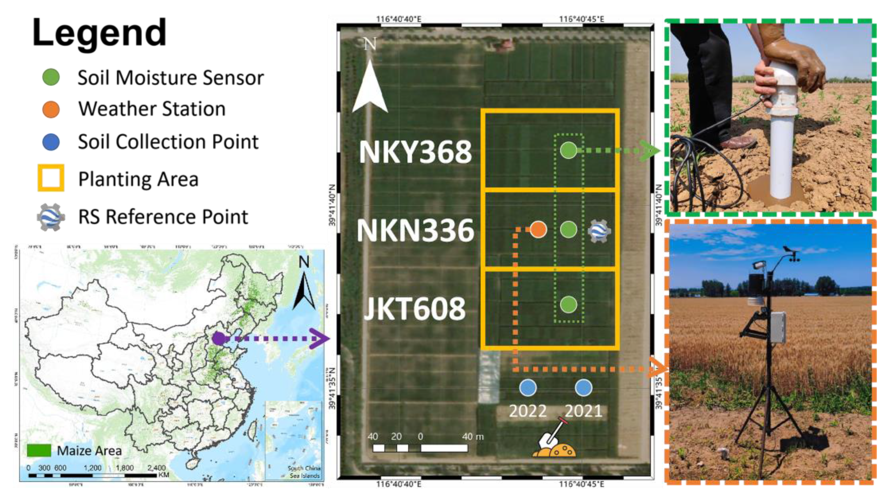
The objective of the study was to assess the feasibility of using “low-cost” multi-source remote sensing and reanalysis data for parameter optimization of the Hydrus-1D model and conduct a comparative analysis with various typical approaches. Two spring maize crops were grown in 2021 and 2022 at the Tongzhou base of the Maize Research Institute, Beijing Academy of Agricultural and Forestry Sciences, China. We collected meteorological, soil, and crop data during the corn growing period and analyzed the soil moisture and evapotranspiration characteristics during maize growth. Five typical methods for soil hydrodynamic parameter acquisition in the Hydrus-1D model were selected to analyze the boundary flux characteristics of the model simulation results and the effect of differences in the parameter acquisition methods on the accuracy of the multi-depth SWC simulations from three perspectives: overall root zone, growth stage, and soil depth.

2. Methods

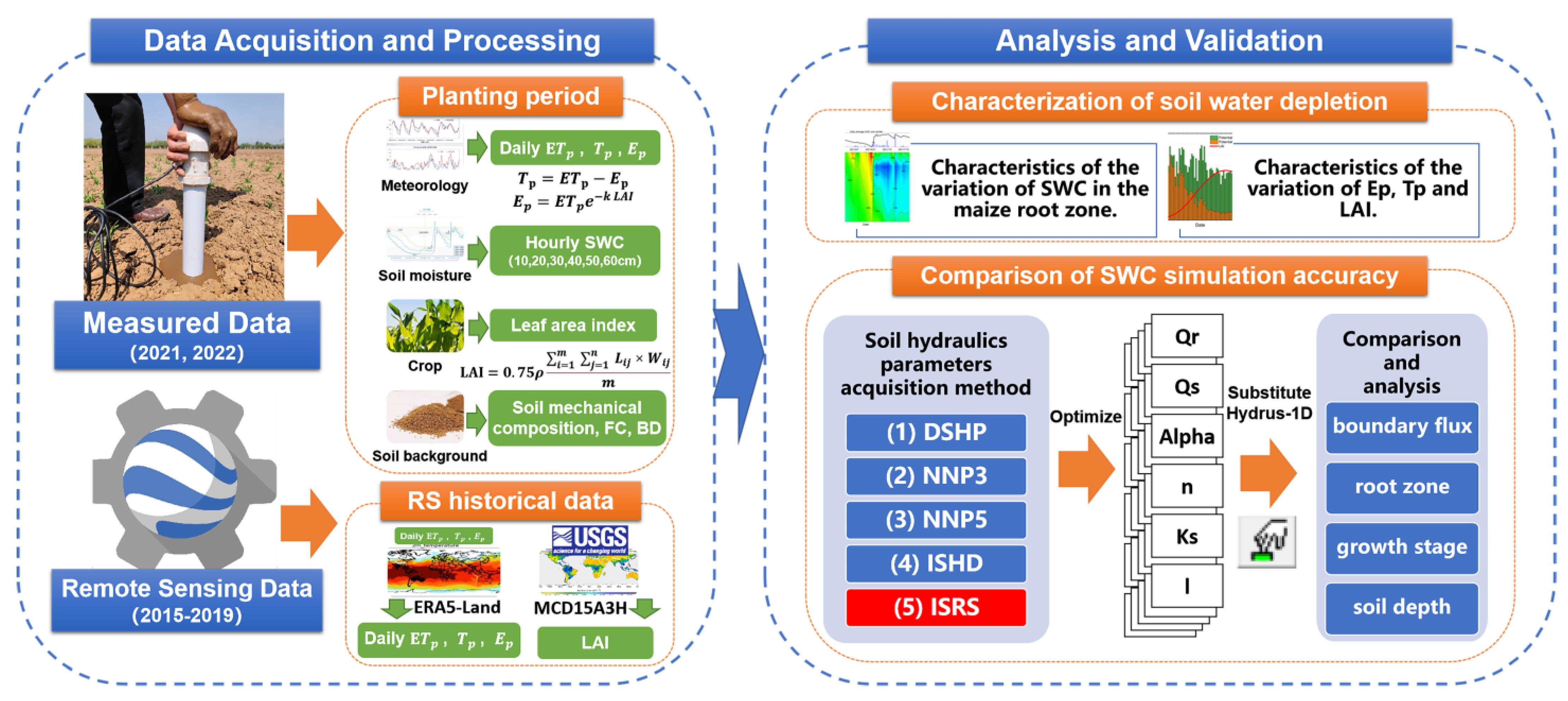
This study aimed to evaluate differences in the accuracy of SWC simulations in the Hydrus-1D model using different methods for soil hydraulic parameter acquisition (Figure 1). By conducting experiments with two corn crops, we collected data on the meteorological environment, soil moisture, crop growth, and soil parameters of the planted fields. The daily potential evapotranspiration, daily potential evapotranspiration, daily potential transpiration rate, and daily leaf area index (LAI) were used as necessary inputs for the simulation of the SWC in the Hydrus-1D model based on the measured data, and then the characteristics of SWC variation and soil water depletion in the root zone profile. Meanwhile, the historical remote sensing dataset was introduced through the GEE platform to obtain the meteorological environment, SWC, and LAI change process for the same period from 2015 to 2019 in the planting field to extend the historical dataset. The soil hydraulic parameters obtained by the five approaches were substituted into the Hydrus-1D model and simulated for each sample. The variation characteristics of the boundary fluxes in the root zone were analyzed to evaluate differences in the simulation accuracy from three perspectives: overall root zone, growth stage, and soil depth.

2.1. Hydrus-1D Model

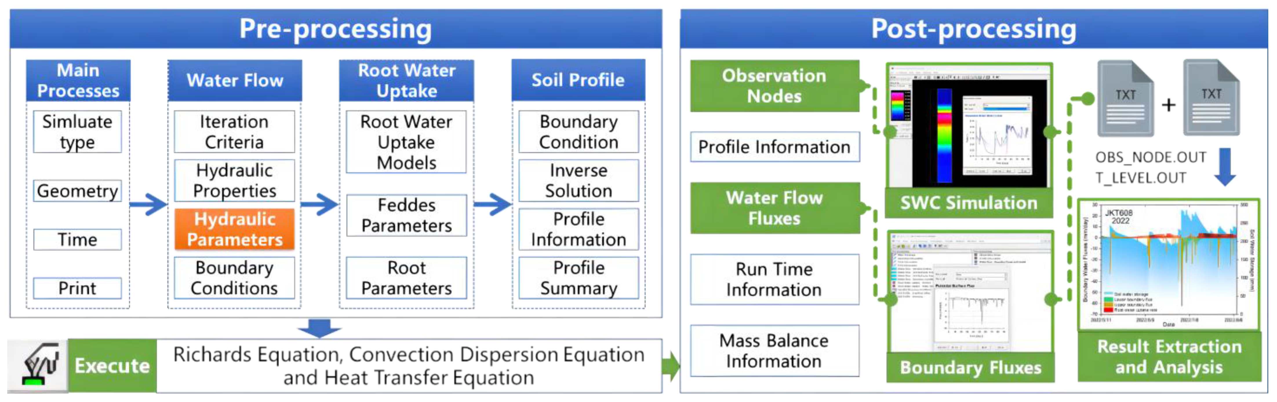
The Hydrus-1D model has a modular design with a preprocessing section for configuring the base parameters, an execution section for carrying out iterative modeling of soil water transport, and a post-processing section providing run results and process information (Figure 2). The model was set up sequentially to progressively configure the model parameters and adjust the subsequent parameter options according to differences in the settings. The core of this study focused on the configuration of the soil hydrodynamic parameters within the water flow module of the preprocessing session. The SWC variation in the maize root zone was simulated by substituting the soil hydrodynamic parameters obtained in different manners. Six observation points at depths of 10, 20, 30, 40, 50, and 60 cm in the soil profile were set up to output the simulation results. By default, the Hydrus-1D model uses centimeters as the base unit of measurement for the input/output. To facilitate comparison, we converted the output results to millimeters as the base unit for analysis and discussion in the Results section. The remaining modules were configured using the parameters recommended by similar studies or the Hydrus-1D model.

• Theoretical equations for water flow motion

Soil moisture in the inclusion zone mainly undergoes one-dimensional vertical soil moisture transport. Therefore, the Richards equation [42] was used to calculate the soil moisture variation in the vertical profile (the axes are positive downward):

$$c\left(h\right)\frac{\partial \mathrm{h}}{\partial \mathrm{t}}=\frac{\partial }{\partial \mathrm{z}}\left[k\left(h\right)\frac{\partial \mathrm{h}}{\partial \mathrm{z}}-k\left(h\right)\right]-s\left(z,t\right),$$

(1)

where $c\left(h\right)$ is the specific water capacity (cm^–1), $t$ is time (d), $k\left(h\right)$ is the soil hydraulic conductivity (cm/d), $h$ is the pressure head (cm), $z$ is the vertical soil depth coordinate (cm), and $s\left(z,t\right)$ is the soil root water uptake rate (cm/d).

The soil moisture characteristic curves were fitted using the van Genuchten model in the Hydrus-1D model [43]:

$$\theta \left(h\right)=\left\{\begin{array}{c}{\theta }_r+\frac{{\theta }_s-{\theta }_r}{{\left[1+|\alpha h{|}^n\right]}^m} h<0\\ {\theta }_s h>0\end{array}\right\},$$

(2)

$$K\left(h\right)=K_s{S}_e^l{\left[1-{\left(1-S_e^{\frac{1}{m}}\right)}^m\right]}^2,$$

(3)

$$m=1-\frac{1}{n},n>1,$$

(4)

where ${\theta }_s$ is the saturated water content (cm³/cm³); ${\theta }_r$ is the residual water content (cm³/cm³); $m$, $\alpha$, and $n$ are empirical shape factors in the water retention function; $K_s$ is the saturated hydraulic conductivity (cm/d); $l$ is the shape factor (pore connectivity parameter) in the hydraulic conductivity function; and $S_e$ is the relative saturation, $S_e=\frac{\theta -{\theta }_r}{{\theta }_s-{\theta }_r}$.

This study focused on six key soil hydraulic parameters in the van Genuchten model: saturated water content (${\theta }_s$, cm³/cm³), residual water content (${\theta }_r$, cm³/cm³), saturated hydraulic conductivity ($K_s$, cm³/d), the inverse of inlet suction ($\alpha$, cm^–3), pore size distribution index ($n$, n > 1), and soil pore connectivity parameter ($l$).

• Calculation of potential transpiration rate

The potential evapotranspiration of the crop ($E{T}_{\mathrm{p}}$) was calculated using the Penman–Monteith (P–M) equation recommended by the FAO [44]. Here, $T_{\mathrm{p}}$ denotes the potential evapotranspiration rate (mm/day), expressed as follows:

$$T_{\mathrm{p}}=E{T}_{\mathrm{p}}-E_{\mathrm{p}}.$$

(5)

$E_{\mathrm{p}}$ was calculated as follows [45]:

$$E_p=E{T}_p{e}^{-k\cdot LAI},$$

(6)

where $LAI$ is the leaf area coefficient (m²/m²) and $k$ is the dimensionless plant canopy radiation attenuation coefficient (0.4) [46].

• Calculation of the water uptake rate of the maize root system

The root water uptake rate can be expressed as the volume of water consumed per unit volume of soil per unit of time. Hydrus-1D uses the Feddes model to simulate the root uptake rate process [47], expressed as follows:

$$S\left(z,t\right)=\alpha \left(h,z\right)\cdot \beta \left(z\right)\cdot T_p$$

(7)

and

$$\alpha \left(h,z\right)=\{\begin{array}{cc}1& h_1\le h<0\\ \frac{h-h_2}{h_2-h_1}& h_2\le h<h_1\\ 0& h\le h_2\end{array},$$

(8)

where $\alpha \left(h,z\right)$ is the water stress response function (dimensionless), $\beta \left(z\right)$ is the standardized root water uptake distribution function (dimensionless), $T_p$ is the potential crop transpiration rate (cm/d), $h_1$ and $h_2$ are the soil water potential at which the root water uptake rate decreases from 1 cm and decreases to 0 cm, respectively.

The crop root water uptake rate was more sensitive to the SWC. Crops can more easily uptake soil water between the soil capillary break water content and the field water holding rate. Crop uptake of soil water is more difficult when the SWC is between the wilting point and soil capillary rupture water content. The parameters of the maize root water-uptake configuration provided by the Hydrus-1D model were chosen for this study [48].

Table 1. Parameter configuration for water uptake rate of maize roots.

Parameters	Value	Definition
P0 (cm)	–15	root suction pressure head
P0pt (cm)	–30	root maximum rate suction pressure head
P2H (cm)	–325	ultimate pressure head
P2L (cm)	–600	pressure head when transpiration rate is r2L
P3 (cm)	–8000	withering point pressure head
r2H	0.5	hourly potential transpiration rate
r2L	0.1	potential transpiration rate

lists the details of the maize root water uptake rate parameters.

• Model boundary parameter configuration

In this study, days were used as the units of the prediction time step. The surface soil of the corn plantation plots was directly exposed to air, and standing water was not produced during rainfall. Therefore, the upper boundary condition was chosen as the atmospheric boundary condition with a surface layer with crop cover:

$$\{\begin{array}{c}\left|-K\frac{\partial h}{\partial x}-K\right|\le E\hfill \\ h_a\le h\le h_s=0\hfill \end{array},x=0,$$

(9)

where $E$ is the maximum potential evaporation or infiltration rate under the current atmospheric conditions, $h_s$ is the maximum allowable surface pressure head under the existing soil conditions, generally set to 0, $h_a$ is the minimum allowable surface pressure head under the current soil conditions, as obtained from the equilibrium conditions between the water vapor and soil water in the atmosphere, and $h_a$ was calculated as follows:

$$h_a=-\frac{RT}{Mg}\ln \left(H_r\right),$$

(10)

where $H_r$ is the air humidity, $M$ is the mass of water molecules, usually set as $M$ = 0.018015 kg/mol, $g$ is the acceleration due to gravity ($g$ = 9.81 m/s²), and $R$ is the universal gas constant [$R$ = 8.314 J/(kg·K)].

The groundwater at the corn plantation plot was deep without groundwater recharge; the plot envelope was in a free drainage state. Therefore, the lower boundary condition of the Hydrus-1D model adopted free drainage.

2.2. Methods for Obtaining Soil Hydraulics Parameters

This study referred to the method used to obtain the soil hydraulic parameters for the Hydrus-1D model in existing studies. Three main acquisition methods were used: default parameters for soil types, predictions from soil mechanical parameters, and inverse solutions from historical data. Five typical soil hydraulic parameter acquisition methods were designed, considering the convenience and cost of parameter acquisition (Figure 3). The estimation of the soil hydraulic parameters using the soil mechanical composition was implemented using a neural network prediction module [32]. This module has a built-in Rosetta transformation dynamic link library (dll) developed by the U.S. Salinity Laboratory [49] based on a neural network approach to estimate soil water retention. Five typical soil hydraulic parameters were obtained using the following methods.

• Default soil hydrodynamic parameters (DSHP) were used to determine the soil texture type. Based on the results of [31], the Hydrus-1D model provided the average soil hydrodynamic parameters for 12 soil texture types as optional default parameters. The soil texture in the root zone of maize in the different years in this study was clay loam (

  Table 2. Mechanical composition of the soil at different depths.

  Year	Depth (cm)	Soil Particle Volume Fraction					Soil Field Capacity (cm3/cm3)	Soil Bulk Density (g/cm3)
  		Sand		Silt		Clay
  		0.25 ≤ Ф < 2 (mm)	0.05 ≤ Ф < 0.25 (mm)	0.02 ≤ Ф < 0.05 (mm)	0.002 ≤ Ф < 0.02 (mm)	Ф < 0.002 (mm)
  2021	10 cm	2.30%	24.82%	19.72%	15.80%	37.36%	33.39%	1.49
  	20 cm	2.40%	26.02%	16.64%	21.88%	33.06%	33.85%	1.52
  	30 cm	2.93%	25.71%	21.80%	19.16%	30.40%	33.26%	1.52
  	40 cm	2.66%	23.50%	21.76%	20.28%	31.80%	33.24%	1.46
  	50 cm	4.01%	28.39%	16.52%	18.72%	32.36%	33.28%	1.51
  	60 cm	3.59%	23.39%	19.84%	19.02%	34.16%	35.18%	1.59
  	Mean	2.96%	25.31%	19.38%	19.14%	33.21%	33.70%	1.52
  2022	10 cm	3.31%	25.04%	20.58%	15.84%	35.23%	33.14%	1.51
  	20 cm	2.90%	24.93%	25.80%	17.30%	29.07%	33.07%	1.53
  	30 cm	3.01%	25.89%	22.38%	18.90%	29.82%	32.54%	1.54
  	40 cm	3.33%	26.71%	18.22%	17.92%	33.82%	33.71%	1.53
  	50 cm	4.09%	29.53%	18.24%	17.30%	30.84%	32.47%	1.54
  	60 cm	4.10%	26.88%	19.14%	17.38%	32.50%	33.36%	1.56
  	Mean	3.45%	26.50%	20.73%	17.44%	31.88%	33.05%	1.54

  ).
• Neural network prediction using three soil mechanical composition parameters (NNP3). Soil particle size ratios (ratios of sand, silt, and clay particles; %) were used to estimate five soil hydraulic parameters (${\theta }_s$, ${\theta }_r$, $K_s$, α, and $n$) for each soil depth. The soil pore connectivity parameter ($l$) was set to the default value of 0.5.
• Neural network prediction using five soil mechanical composition parameters (NNP5). Five soil hydraulic parameters (${\theta }_s$, ${\theta }_r$, $K_s$, α, and $n$) were estimated for each soil depth using the soil particle size ratio (ratio of sand, silt, and clay particles; %), soil field water capacity (SWC at 33 kPa; %), and soil bulk density (g/cm³) as inputs. The soil pore connectivity parameter ($l$) was set to 0.5.
• Inverse solutions from measured historical data (ISHD). We selected all measured data (meteorological, soil moisture, and LAI) from the JKT363 plot during the growth period for the inverse solution of the six soil hydraulic parameters (${\theta }_s$, ${\theta }_r$, $K_s$, α, $n$, and $l$). The initial values of each parameter were set to the default values for the clay loam soil texture. The inverse solution module of Hydrus-1D allows the optimization of a maximum of 15 parameters; simultaneous optimization of excessive parameters is not recommended [50]. A hierarchical approach was used to optimize the parameters. The soil depths were optimized from shallow to deep in the order of six parameters for that layer depth; the default parameters were replaced with the optimized parameters.
• Inverse solution from historical remote sensing data (ISRS). This process was the same as that of the historical data inverse solution process. Remote sensing data were used instead of measured historical data for inverse parameter solutions. This is because the division of the soil depth in the reanalysis data is difficult to match with that of the SWC sensor. We regarded the depth of 0–100 cm as a whole. Only one inverse solution was performed for each year of remote sensing data.

2.3. Model Evaluation Metrics

As suggested by [51], three classic error indicators were chosen to evaluate the accuracy of the model to facilitate a comparison of the simulation accuracy of the Hydrus-1D model in different studies.

The mean absolute error (MAE):

$$MAE=\frac{1}{m}{{\displaystyle \sum }}_{i=1}^m\left|\left(y_i-\stackrel{\wedge }{y_i}\right)\right|.$$

(11)

The mean squared error (MSE):

$$MSE=\frac{1}{m}{{\displaystyle \sum }}_{i=1}^m{\left(y_i-\stackrel{\wedge }{y_i}\right)}^2.$$

(12)

The root mean squared error (RMSE):

$$RMSE=\sqrt{\frac{1}{m}{{\displaystyle \sum }}_{i=1}^m{\left(y_i-\stackrel{\wedge }{y_i}\right)}^2}.$$

(13)

In the above formulas, $\stackrel{\wedge }{y_i}$ is the predicted value, $y_i$ is the true value, and $\overline{y_i}$is the average value. The MAE reflects the actual situation of the predicted error value. The MSE is the expected value of the square of the difference between the estimated and observed values, which can evaluate the degree of change in the data. The smaller the MSE value, the better the accuracy of the prediction model. The RMSE is the arithmetic square root of the MSE.

2.4. Model Implementation and Analysis

Version 4.17 of the Hydrus-1D model was used in this study. This version of the software can be downloaded and used for free from the Hydrus website (https://www.pc-progress.com, accessed on 10 August 2021). Origin Pro (version 2022a) was used for data analysis and graphing; SPSS Statistics 24.0 was used for LAI function fitting. The Anaconda platform was used as the base platform for evaluating the accuracy of the simulated data. The underlying Python version was 3.7.

3. Experimental Area

The planting trials for this study were conducted at the Tongzhou base at the Maize Research Institute, Beijing Academy of Agricultural and Forestry Sciences (39°41′25″–39°41′41″N, 116°40′39″–116°41′25″E) (Figure 4). The experimental site is located in an area with flat topography and a deep groundwater level, which has a warm, temperate, semi-humid, semi-arid monsoon climate. The average annual temperature is 11.3 °C and the precipitation is 620 mm, of which 65% is concentrated in July and August. The annual sunshine hours are 2435.4 h, with abundant light and heat resources. Two spring maize planting trials were conducted from 15 April to 27 July 2021, and 1 May to 8 August 2022. Three planting plots were set up for each crop, with three characteristic corn varieties: NKY368, NKN336, and JKT608, respectively. Soil moisture content sensors and meteorological monitoring stations were deployed in the central areas of the plots. The equipment was installed after maize planting and was removed before harvest to avoid disrupting farm machinery operations. Considering that the soil moisture sensor requires a stabilization period after installation to achieve accurate measurements, data from 10 May to 27 July 2021 and 11 May to 8 August 2022 were intercepted for analytical validation in this study. The planting density of maize in all plots was 40 cm between the plants and 60 cm between the rows. Agronomic measures were performed according to the experience of the professional agronomists at the base. There was no active irrigation during the time frame covered in this study. Rainfall can be considered the only source of moisture for the soils in this study.

4. Data Acquisition and Analysis

4.1. Acquisition and Processing of Measured Data

• Soil background data

Soil samples were collected from planting plots at depths of 10, 20, 30, 40, 50, and 60 cm using the ring knife method in 2021 and 2002. Three replicate samples were collected from each soil depth. The soil particle volume fraction, soil field water-holding capacity, and soil bulk density of the soil samples were measured separately. The mechanical compositions of the soil samples for both crops were relatively similar. Table 2 lists the average soil mechanical composition for each depth sample. Based on the international soil texture classification standard [52], the soil texture classification triangle [53] of the USDA was used to evaluate that all soil types at different depths were clay loam. The soil texture in the root zone of maize was highly consistent. The average soil field water-holding capacity of the planted plots was 33.37% and the average bulk density was 1.53 g/cm³.

• Soil moisture data

One set of fixed soil moisture monitoring stations was installed at the center of each planting plot and three sets of soil moisture monitoring equipment were deployed. Soil moisture data were collected using a tubular soil moisture sensor (WEITU Fleb-30c, Shenyang, China) based on the FDR principle. Six layers of soil volumetric water content (%) were collected at soil depths of 10 (SVWC10), 20 (SVWC20), 30 (SVWC30), 40 (SVWC40), 50 (SVWC50), and 60 cm (SVWC60), with a collection frequency of 1 h. Data were transmitted via a 4G wireless communication network and stored in a cloud database. The soil volumetric water content (%) at each depth was obtained by averaging the hourly data for each day.

• Meteorological data

One set of automatic meteorological monitoring stations was installed at the center of the planting area to collect data on the air temperature (T, °C), relative air humidity (RH, %), cumulative daily rainfall (Pr, mm), surface atmospheric pressure (P, hPa), wind speed (U2, m/s), and net surface radiation (Rn, MJ/m²). Meteorological data were transmitted back to the data cloud and stored in the database via a 4G wireless communication network with a collection frequency of 1 h. The rainfall data were taken as the daily maximum, and the remaining indicators were converted from hourly to daily data by taking the average. Daily ETp was calculated using the FAO ET₀ Calculator (version 3.2) [54].

• Leaf area index data

Five standard maize plants were fixed near the soil moisture sensor in each planting plot (15 plants per crop). The plant height and leaf parameters were collected weekly from 1 June 2021 to 14 July 2021 and from 6 June 2022 to 18 July 2022 for the fixed plants. Leaf area data were collected seven times per planting cycle. The length and width of all the leaves from each standard maize plant were measured using a straightedge. The maize LAI was calculated as follows [55]:

$$\text{LAI}=0.75\rho \frac{{\Sigma }_{i=1}^m{\Sigma }_{j=1}^n{l}_{ij}\times w_{ij}}{m},$$

(14)

where 0.75 is the correction factor of the maize leaf area, $\rho$ is the density of the maize plant (plant/m²), $m$ is the number of measured plants, and $L_{ij}$ and $W_{ij}$ are the length and maximum width of the j-th leaf of the i-th maize plant (cm), respectively.

The LAI shows a “slow growth–fast growth–slow decline” during maize growth [55]. Therefore, in this study, a modified logistic equation was used to simulate the dynamics of the LAI of spring maize [56]:

$$y=\frac{a}{1+\exp \left(b+c\times t+d\times t^2\right)},$$

(15)

where $y$ is the LAI; $t$ is the number of days after seedling emergence; and $a$, $b$, $c$, and $d$ are the parameters.

Table 3. Results of the parameter fitting for the LAI equation.

Year	Variety	Equation Parameters				R2
		$\mathit{a}$	$\mathit{b}$	$\mathit{c}$	$\mathit{d}$
2021	NKY368	16.8894	8.9255	–0.2303	0.0016	0.9802 *
	NKN336	11.0794	9.2782	–0.2605	0.0019	0.9907 *
	JKT608	4.6855	10.2934	–0.3352	0.0024	0.9968 *
2022	NKY368	8.9247	9.8351	–0.2935	0.002	0.9979 *
	NKN336	5.5897	9.9825	–0.3189	0.0022	0.9997 *
	JKT608	4.3050	11.7665	–0.3913	0.0026	0.9996 *

* Indicates a significant correlation at the 0.05 level.

lists the results for the parameter fitting of the modified logistic equations. The goodness-of-fit, $R^2$, for all the results exceeded 0.98 and was significant at the 0.05 level. The fitted curve equations accurately reflected the real LAI variation process for different maize varieties.

• Maize phenological data

The entire maize planting process was tracked. The nodal dates for the crop growth characteristics, such as sowing, seedling emergence, male extraction, pollen dispersal, and spatulation, were recorded separately for the maize planting plots. Referring to the criteria of [8] for dividing the maize growing period, the entire growing period was divided into three stages: seedling, tassel, and anthesis maturity.

Table 4. Division of growth stages of the two maize crops.

Year	Seedling Stage	Tassel Stage	Anthesis Maturity Stage	Total Days
2021	04/15–5/18	05/19–6/13	06/14–7/27	103
2022	05/01–5/29	05/30–6/24	06/25–8/8	99

lists the division of the growth stages over the two years of planting. The entire growing period days were similar for both cropping processes; the overall growth period was shorter in 2022.

4.2. Remote Sensing Data Acquisition and Processing

This study aimed to use long time-series remote sensing data instead of ground monitoring site-measured data for the inverse solution of the soil hydrodynamic parameters. Remote sensing data were obtained using the GEE platform. The querying, analysis, and downloading of the long time-series data were implemented in the Coder Editor tool provided by the GEE platform using the Python language. The time range was chosen to cover the period from 10 May 2015 to 8 August 2019. The coordinates of the centroid of the planting plot (116.6794°E, 39.6942°N) were used to obtain spatially located matched image element values for consecutive time steps. The hourly ERA5-Land dataset [40] was used for the historical, meteorological, and SWC data. ERA5-Land is a reanalysis dataset that provides a consistent view of the evolution of land variables over several decades at an enhanced resolution compared with ERA5. ERA5-Land was produced by replaying the land component of the ECMWF ERA5 climate reanalysis data. Reanalysis combines model data with observations from across the world into a globally complete and consistent dataset using the laws of physics. Reanalysis produces data across several decades, providing an accurate description of the past climate. LAI data were obtained using the MODIS Level 4 product MCD15A3H (Version 6.1) [57]. MCD15A3H is a 4-day composite dataset with a 500-m pixel size. The algorithm selected the best pixel available from all the acquisitions of both MODIS sensors located on NASA’s Terra and Aqua satellites within the 4-day period.

Table 5. Detailed parameters for the remote sensing data indicators.

Source	Name	Units	Resolution	Scale Factor	Description
	dewpoint_temperature_2 m	K	0.1° × 0.1°	1	2 m dew point temperature
ERA5-Land	temperature_2 m	K	0.1° × 0.1°	1	Temperature of air at 2 m above land surface
	u_component_of_wind_10 m	m/s	0.1° × 0.1°	1	Eastward component of the 10 m wind
	v_component_of_wind_10 m	m/s	0.1° × 0.1°	1	Northward component of the 10 m wind
	surface_pressure	Pa	0.1° × 0.1°	1	Pressure of the atmosphere on the surface
	total_precipitation	m	0.1° × 0.1°	1	Large-scale precipitation and convective precipitation
	surface_net_solar_radiation	J/m2	0.1° × 0.1°	1	Amount of solar radiation reaching the surface minus the amount reflected
	volumetric_soil_water_layer_1 (SVWC1)	m3/m3	0.1° × 0.1°	1	Volume of water in soil layer 1 (0–7 cm)
	volumetric_soil_water_layer_2 (SVWC2)	m3/m3	0.1° × 0.1°	1	Volume of water in soil layer 2 (7–28 cm)
	volumetric_soil_water_layer_3 (SVWC3)	m3/m3	0.1° × 0.1°	1	Volume of water in soil layer 3 (28–100 cm)
MCD15A3H	Lai_500m	m2/m2	500 m	0.1	4-day composite data set with 500-m pixel size

lists information for the field names, units, spatial resolution, scaling, and description of the acquired remote sensing history data.

The raw data acquired must be processed for subsequent use. The units of the air temperature data must be converted from K to °C, units for the surface pressure data must be converted from Pa to hPa, units for rainfall data must be converted from m to mm, and units for the net surface radiation data must be converted from J/m² to MJ/m². Data from ERA5-Land must be converted from hourly to daily intervals; the rainfall was taken as the daily maximum, and the rest of the indicators were taken as the average. The LAI data were converted from 4-day intervals to daily data using data interpolation.

4.3. Soil Hydraulic Parameter Benchmarks

Table 6. Soil hydraulic parameters obtained by multiple methods.

Method	Year	Depth (cm)	${\mathit{\theta }}_{\mathit{r}}({\mathbf{cm}}^3/{\mathbf{cm}}^3)$	${\mathit{\theta }}_{\mathit{s}}({\mathbf{cm}}^3/{\mathbf{cm}}^3)$	$\mathit{\alpha }$	$\mathit{n}$	${\mathit{K}}_{\mathit{s}}({\mathbf{cm}}^3/\mathbf{d})$	$\mathit{l}$
DSHP	1988	10–60 cm	0.0950	0.4100	0.0190	1.31	6.24	0.50
NNP3	2021	10 cm	0.0869	0.4517	0.0130	1.37	8.57	0.50
		20 cm	0.0831	0.4444	0.0112	1.42	9.96	0.50
		30 cm	0.0804	0.4402	0.0099	1.46	11.36	0.50
		40 cm	0.0828	0.4468	0.0098	1.45	11.78	0.50
		50 cm	0.0810	0.4360	0.0126	1.41	7.19	0.50
		60 cm	0.0846	0.4487	0.0113	1.42	10.47	0.50
		Average	0.0831	0.4446	0.0113	1.42	9.89	0.50
NNP3	2022	10 cm	0.0849	0.4471	0.0124	1.40	8.60	0.50
		20 cm	0.0792	0.4391	0.0090	1.48	12.10	0.50
		30 cm	0.0797	0.4388	0.0097	1.47	11.50	0.50
		40 cm	0.0831	0.4422	0.0123	1.41	8.04	0.50
		50 cm	0.0792	0.4320	0.0124	1.42	7.10	0.50
		60 cm	0.0816	0.4389	0.0120	1.42	8.06	0.50
		Average	0.0812	0.4396	0.0113	1.43	9.23	0.50
NNP5	2021	10 cm	0.0795	0.4207	0.0123	1.31	6.76	0.50
		20 cm	0.0767	0.4112	0.0090	1.36	4.70	0.50
		30 cm	0.0742	0.4074	0.0080	1.40	5.04	0.50
		40 cm	0.0766	0.4228	0.0087	1.40	7.45	0.50
		50 cm	0.0750	0.4119	0.0098	1.35	5.36	0.50
		60 cm	0.0779	0.3991	0.0081	1.35	2.37	0.50
		Average	0.0766	0.4121	0.0093	1.36	5.28	0.50
NNP5	2022	10 cm	0.0772	0.4134	0.0113	1.33	5.73	0.50
		20 cm	0.0728	0.4033	0.0074	1.42	4.99	0.50
		30 cm	0.0720	0.4001	0.0086	1.39	4.83	0.50
		40 cm	0.0763	0.4090	0.0099	1.34	4.51	0.50
		50 cm	0.0719	0.4011	0.0101	1.35	4.79	0.50
		60 cm	0.0741	0.3996	0.0096	1.34	3.76	0.50
		Average	0.0741	0.4044	0.0095	1.36	4.76	0.50
ISHD	2021	10 cm	0.0968	0.3437	0.0190	1.31	5.47	0.25
		20 cm	0.0516	0.3921	0.0127	1.73	8.46	0.26
		30 cm	0.0710	0.3850	0.0149	1.40	5.42	0.38
		40 cm	0.0496	0.3780	0.0151	1.32	7.96	0.27
		50 cm	0.0873	0.3729	0.0141	1.34	8.93	0.40
		60 cm	0.1193	0.3621	0.0113	1.32	4.99	0.44
		Average	0.0793	0.3723	0.0145	1.40	6.87	0.33
ISRS	2019	10–60 cm	0.0838	0.4503	0.0049	1.44	9.80	0.65
	2018	10–60 cm	0.0853	0.4391	0.0069	1.40	11.38	0.76
	2017	10–60 cm	0.0842	0.4535	0.0074	1.45	8.68	0.64
	2016	10–60 cm	0.0870	0.4381	0.0049	1.44	11.73	0.91
	2015	10–60 cm	0.0834	0.4425	0.0087	1.42	10.75	0.65
	Average	10–60 cm	0.0847	0.4447	0.0065	1.39	10.47	0.72

lists the parameter values obtained from five typical soil hydraulic parameter acquisition methods, which were substituted into the Hydrus-1D model to simulate SWC variation in different plots. As the soil type in the root zone of the planted plots in this study was clay loam, the DSHP method used the same hydraulic parameters for the root zone soil from 10 to 60 cm. The NNP3 and NNP5 methods used neural network estimation for each depth based on the measured soil mechanical composition data (Table 2) from soil samples collected over two years; the default value of 0.5 was used for $l$. The differences in the hydraulic parameters between different depths were small. The ISHD approach was inversely solved using historical data from the JKT608 plot in 2021; the parameters at different depths had notable differences. The parameters obtained by inversely solving for different years using the ISRS approach were similar.

4.4. Data Analysis

• Statistical characteristics of the environment in the maize-growing areas

Table 7. Statistics of the environmental indicators in the maize growing areas.

Indicator	Unit	2021					2022
		Mean	SD	Min	Median	Max	Mean	SD	Min	Median	Max
SVWC10	%	25.66	6.73	8.02	26.06	38.50	24.71	4.56	13.07	25.28	33.07
SVWC20	%	27.92	5.74	13.90	28.76	38.43	31.12	5.19	15.91	32.73	39.95
SVWC30	%	27.24	4.55	14.93	28.03	36.46	33.26	3.77	20.98	34.62	38.29
SVWC40	%	28.02	4.55	16.33	29.52	35.50	34.17	2.48	26.45	34.35	38.35
SVWC50	%	28.24	4.01	17.90	28.37	35.49	33.39	1.78	29.00	33.79	36.83
SVWC60	%	28.16	3.73	19.40	28.60	36.18	32.21	1.65	27.91	32.47	35.78
T	°C	25.21	3.12	16.08	25.62	30.56	25.71	3.43	15.80	26.67	31.25
RH	%	60.08	20.01	18.49	62.25	94.61	69.28	17.26	27.43	75.15	98.95
Pr	mm	4.48	11.66	0	0	73.80	4.93	12.53	0	0	87.60
U2	m/s	2.37	0.80	0.89	2.26	4.80	2.33	0.71	1.21	2.17	4.99
Rn	MJ/m2	12.66	3.71	2.68	13.03	17.87	13.37	3.54	3.58	14.45	17.55
P	hPa	1003.29	4.28	988.95	1002.39	1010.76	1005.30	4.37	994.95	1005	1017.38
ETp	mm	4.56	1.10	2.40	4.30	7.30	4.84	0.91	1.80	4.80	7.30

lists the statistical results for the measured data during the maize growing process, including the mean, standard deviation (SD), minimum (min), median, and maximum (max) values. Overall, the environmental differences between the two crops were insignificant. Particularly, the average daily precipitation, average daily temperature, and average daily net surface radiation were 0.45 mm, 0.5 °C, and 0.71 MJ/m² higher in 2022 compared to 2021, respectively, during the maize growing season, which indirectly led to higher average daily root zone SWC and average daily ETp in 2022.

• Statistical characteristics of remote sensing data in maize growing areas

Table 8. Statistics on the remote sensing data indicators for the maize growing areas (2015–2019).

Indicator	Unit	Mean	SD	Min	Median	Max
SVWC1	%	23.72	9.08	12.12	21.42	42.51
SVWC2	%	22.05	8.48	13.40	18.65	41.67
SVWC3	%	18.45	3.93	14.30	17.10	30.52
Tdew	°C	15.45	7.36	–10.80	16.42	26.98
Tmean	°C	26.25	3.46	10.37	26.52	34.51
Rn	MJ/m2	13.10	3.92	1.22	14.41	17.75
U2	m/s	2.38	0.81	0.63	2.26	5.12
Pr	mm	6.70	13.73	0	1.00	122.00
RH	hPa	1003.94	4.25	992.97	1003.82	1018.14
LAI	m2/m2	1.25	0.41	0.30	1.20	2.30

lists the results for the statistical analysis of the meteorological, soil moisture, and LAI data obtained from 10 May to 8 August 2015 to 2019. Compared with the measured data statistically obtained in Table 7, the statistical results for Tmean, Rn, RH, and U2 were more similar, while the average daily precipitation was approximately 1.99 mm higher.

• Characteristics of SWC variation in the maize root zone

Figure 5 shows the variation in the SWC in the root zone profiles of different plots. The overall trend in the SWC in the root zones of the different plots in the same year was highly consistent. The differences in the absolute values of the SWC at the same time point in different plots may have been influenced by differences in the soil texture, crop growth, and other factors. Soil moisture sensors were sufficiently sensitive to capture the changes in the SWC from rainfall. The overall soil moisture content was significantly higher in 2022 than that in 2021, which is consistent with the findings from the meteorological statistics in Table 7.

• Characteristics of evapotranspiration and LAI changes during maize cultivation

Figure 6 shows the variation in the Ep, Tp, and LAI in each plot for the two crops. The ETp values of different varieties in the same year remained consistent because the same meteorological data were used to calculate them. Changes in the LAI determine the differentiation between the Ep and Tp. With an increase in the LAI, there was a gradual increase in the proportion of Tp to ETp. The LAI reached its maximum value from approximately 73 to 85 days after sowing and declined slowly thereafter. The maximum percentage of Tp was 92% when the LAI reached its maximum (NKY368); the transpiration of plants became the main pathway of soil water consumption. The maximum LAI values were significantly different among different varieties. The ranking of the maximum LAI (LAI_max) was: NKY368 (LAI_max = 6.40 m²/m²) > NKN336 (LAI_max = 4.63 m²/m²) > JKT608 (LAI_max = 4.09 m²/m²).

5. Results and Discussion

5.1. Water Boundary Flux Characteristics of the Maize Root Zone

Figure 7 shows the actual daily upper boundary flux (vTop), actual lower boundary flux (vBot), actual root water uptake (vRoot), and soil water storage (SWS) for different plots of the Hydrus-1D model under the NNP5 parameter acquisition method. The upper boundary flux mainly reflects infiltration (−) and evaporation (+) at the surface soil boundary. The lower boundary flux mainly reflects groundwater recharge (+) and deep infiltration of bottom drainage (–). The actual transpiration rate was calculated based on the daily Tp, root distribution, and actual SWC conditions. The SWS reference [33] method was used to convert the root zone water layer thickness (mm) based on the actual SWC at different depths. Overall, the boundary moisture flux characteristics were nearly identical between plots in the same year. The mean values of the cumulative vTop, cumulative vBot, cumulative vRoot, and SWS changes ($\Delta SWS$) across plots during the 2021 planting were –246.83, –145.29, 145.77, and –51.36 mm, respectively. In 2022, these were –320.83, –137.67, 200.17, and –0.03 mm, respectively. Evapotranspiration was the main pathway involved in soil water depletion. The total actual evapotranspiration accounted for 68.26 (2021, Ep = 95.82 mm, Tp = 145.77 mm) and 69.43% (2022, Ep = 108.10 mm, Tp = 200.17 mm) of the total precipitation. Root water uptake from crop transpiration accounted for 60.34 and 64.93% of the total actual evapotranspiration in 2021 and 2022, respectively.

The water inflow/outflow process can be visualized by the variation in the water boundary fluxes in the root zone of maize. Under the environmental conditions in this study, precipitation was the only source of water input. The lower boundary fluxes were all negative owing to the absence of groundwater recharge. Precipitation effectively replenished the soil water storage when the SWC was low (23 June 2021 and 1 July 2022). However, when the SWC approached saturation (12 July 2021 and 3 July 2022), excess precipitation was drained by seepage through the lower boundary. Consistent with the ratio of Ep to Tp for the potential evapotranspiration shown in Figure 6, soil water was consumed mainly by soil evaporation in the early stage. With the change in the maize LAI, crop root uptake gradually became the main pathway in the later stage. On several dates with high precipitation (5 July 2021, 12 July 2021, and 3 July 2022), the water uptake by maize roots dropped to approximately 0 mm. According to the Feddes crop root uptake theory [47], the soil water potential can significantly affect the crop root uptake rate. When the SWC in the root zone of maize reaches or exceeds the soil field water-holding capacity due to heavy precipitation, soil permeability becomes poor, thus preventing the crop uptake of soil water.

5.2. Comparison of Accuracy of Parameter Acquisition Methods for Estimating Overall Root Zone SWC

Table 9. Accuracy of soil moisture simulations in the root domain via different hydrodynamic parameter acquisition methods.

Method	Year	Variety	MSE (%)	MAE (%)	RMSE (%)
NNP5	2021	NKN336	28.04	4.24	5.27
		NKY368	26.27	3.84	4.99
		JKT608	33.28	4.73	5.42
	2022	NKN336	33.19	4.95	5.60
		NKY368	41.04	5.47	6.25
		JKT608	29.89	4.48	5.31
	Average		31.95	4.62	5.47
ISRS	2021	NKN336	27.51	4.16	5.22
		NKY368	27.38	3.93	5.11
		JKT608	25.68	3.97	4.79
	2022	NKN336	41.31	4.97	6.03
		NKY368	51.78	5.55	6.76
		JKT608	29.13	4.07	4.95
	Average		33.80	4.44	5.48
NNP3	2021	NKN336	28.52	4.10	5.31
		NKY368	32.29	4.28	5.54
		JKT608	30.49	4.34	5.20
	2022	NKN336	35.89	5.08	5.88
		NKY368	44.49	5.18	6.06
		JKT608	36.52	5.04	5.94
	Average		34.70	4.67	5.66
ISHD	2021	NKN336	41.60	5.27	6.31
		NKY368	28.48	4.43	5.14
		JKT608	Data were used for inverse solution of the parameters.
	2022	NKN336	37.59	5.01	5.77
		NKY368	35.55	4.86	5.66
		JKT608	40.13	4.83	5.53
	Average		36.67	4.88	5.68
DSHP	2021	NKN336	41.73	5.09	6.38
		NKY368	55.42	5.59	7.33
		JKT608	43.16	5.19	6.11
	2022	NKN336	40.28	5.38	6.27
		NKY368	49.57	5.89	6.94
		JKT608	41.97	5.39	6.39
	Average		45.36	5.42	6.57

lists the accuracies of SWC simulations in the root zone of different plots after the soil hydraulic parameters obtained by the different methods were introduced into the Hydrus-1D model. Using the average RMSE of each plot simulation for the two planting processes, the simulation accuracy of the different soil hydraulic parameter acquisition methods was ranked as NNP5 (RMSE = 5.47%) > ISRS (RMSE = 5.48%) > NNP3 (RMSE = 5.66%) > ISHD (RMSE = 5.68%) > DSHP (RMSE = 6.57%). Among the results, the ISRS approach based on remote sensing had the lowest simulated RMSE of 4.79% for the 2021 crop in the JKT608 plots. In contrast, the DSHP approach with only the default parameters achieved the highest simulated RMSE of 7.33% in the NKY368 plots for the 2021 crop. Using the same parameter acquisition method, the simulation accuracy among the different varieties of plots was ranked as follows: JKT608 (RMSE = 5.52%) > NKN336 (RMSE = 5.80%) > NKY368 (RMSE = 5.98%). There was no significant difference in the simulation accuracy between plots of different maize varieties.

Among all the results, the mean RMSE of the Hydrus-1D model for the SWC simulations in the maize root zone was within 4.79–7.33%. Existing studies usually directly consider the simulation results of the Hydrus-1D model as true values and do not discuss the simulation errors. In similar studies, the RMSE of the SWC simulation results for a watermelon growing area was approximately 9% [22], the RMSE of SWC simulations for the root zone of winter wheat and summer maize in Henan Province, China, was approximately 10% [58], and the RMSE of SWC simulations for rice fields was within 9.6% [59]. Therefore, we suggest that the simulation accuracy of the Hydrus-1D model in this study was acceptable for the different hydraulic parameter acquisition methods.

Among the different methods for obtaining the soil hydrodynamic parameters, the SWC simulation accuracy was the lowest with the default soil hydrodynamic parameters. This is because the default parameters for the clay loam soil type were obtained from the average of thousands of curves for that soil type [19], such that it is difficult to accurately reflect the soil hydraulic properties under specific conditions. The predicted soil hydraulic parameters using three and five soil mechanical composition parameters can further restore the actual soil properties; the physical model can achieve a better fitting accuracy with an increase in the number of parameters involved in the prediction. Notably, the inverse solution of the soil hydrodynamic parameters using remote sensing historical data could obtain almost the best performance in model simulation accuracy. This may be due to the inherently high reliability and consistency of the remote sensing data, which could effectively reflect the real water cycle. The ERA5-Land reanalysis dataset was a further enhancement of the ERA5 dataset, with improved spatial and temporal resolution, numerical accuracy, and enhanced performance for the SWC data, rendering it the most advanced global-scale reanalysis dataset available for terrestrial applications [60]. The authors of [61], using data from 1411 ground-based SWC monitoring sites in China, showed that ERA5-Land can effectively reflect true SWC variation (R = 0.45). Another study [62] showed that the ERA5-Land reanalysis dataset can be used instead of ground-based observations in areas where meteorological data are challenging to obtain. The LAI metrics of the MCD15A3H dataset were likewise shown to be capable of good spatial and temporal resolution and reliability on a global scale [63]. The promising results obtained from remote sensing data used in this study provide a possibility for applying the Hydrus-1D model for SWC simulation forecasting in a unified framework at the global scale.

The ISHD approach improved the simulation accuracy compared to the DSHP approach. However, the simulation accuracy of the ISHD approach was only comparable to that of NNP3; it consumed the entire growth period of the measured data for the parameter inverse solution. Figure 8 compares the SWC simulation results for the parameters of the ISHD approach inverse solution on JKT608. The average MAE and RMSE were 3.88% and 4.47%, respectively, when using the corrected parameters to simulate the SWC in the root zone. The simulation accuracy exceeded all the results listed in Table 9. The parameters for the inverse solution using historical data improved the simulation accuracy significantly for itself, whereas the improvement was limited for other points and years. Differences may have influenced this in the water consumption characteristics of the different crop species (Figure 6). Additionally, the soil sensors were removed after harvest in 2021 and repositioned after seeding in 2022, which also may have led to differences in the soil hydraulics at the same sites in different years, making it difficult to validate the inverse solution parameters for the following year.

5.3. Accuracy Comparison of Parameter Acquisition Methods for Estimating SWC at Different Maize Growth Stages

Figure 9 shows the daily MAE curves of the Hydrus-1D model for SWC simulations in the maize root zone under different methods and the amount of change in the MAE compared with the previous day. Among all the records, the NNP3 approach had the most significant simulation error of 12.51% on 11 July 2021. The lowest MAE values for all modes, except the ISHD, occurred on the first day of the simulation. In terms of typical processes, the SWC showed a typical receding process between 10 May and 23 June 2021, during which there was only a small amount of precipitation. The simulated MAE of each method accumulated slowly with the receding water process; the daily increment in the MAE did not exceed 1%. The daily MAE increments showed a dramatic effect from precipitation on the accuracy of the Hydrus-1D simulations. Almost all dates with MAE increments above 2% had a precipitation process; the MAE decreased sharply on the following day.

Figure 10 shows the error distribution for each growth stage in the form of a box plot. Overall, the accuracy of the model simulations at different growth stages was ranked as follows: seedling stage (MAE = 3.29%) > tassel stage (MAE = 4.68%) > anthesis maturity stage (MAE = 5.52%). In both the seedling and tassel stages, the ISRS method based on remote sensing data had the smallest median MAE (1.88 and 3.25%, respectively) and achieved the best simulation accuracy. In the anthesis maturity stage, the ISHD had the best performance, with a median MAE of 4.35%. The other modalities did not show significant differences at the different growth stages. The simulation errors tended to increase with the development of the growth stages.

To further clarify the effect of different environmental variables on the SWC simulation error of the Hydrus-1D model, we calculated the correlation coefficients between each indicator (meteorology, soil, crop, and parameter acquisition method) and the MAE on a daily basis using the Pearson correlation method [64]. The number of maize sequences after sowing (DOY) was added as an indicator to assess the potential for error accumulation. Figure 11 shows the results of the correlation analysis. The top six highest absolute values of the average correlation coefficients among all the indicators were DOY (R = 0.42) > LAI (R = 0.40) > RH (R = 0.34) > T (R = 0.30) > Rn (R = −0.22) > Pr (R = 0.21). Both the DOY and LAI could reflect information on the prediction duration; therefore, the prediction error of the Hydrus-1D model could be cumulative, where the error increases with an increase in the simulation duration. Similarly, a previous study [58] showed a trend of increasing errors in the Hydrus-1D model simulation of the SWC in the root zone of maize during the growing season. At the same time, the increase in the LAI also implies an increase in the intensity of root water uptake; the complexity of water uptake in maize roots exacerbates the difficulty of model simulation. Here, RH, T, and Rn are all calculated parameters of ETp, which directly determine the intensity of water consumption in soil and crops and indirectly affect the simulation accuracy of the model. The Pr did not show high correlation coefficients due to the fact that precipitation was a small probability discrete event in the planting process, and it was difficult to reflect its importance through correlation coefficients of continuous data. Similar conclusions have been obtained in other studies on SWC prediction in the maize root zone [7,8,65]. The correlation between the soil moisture content and model simulation errors was low and did not show a clear trend. The correlation between the errors of each parameter acquisition method was high; only the correlation between the simulation errors of the ISHD method and other methods was slightly lower (R = 0.45), which is consistent with the error variation process shown in Figure 9.

5.4. Accuracy Comparison of SWC Estimation at Different Depths for each Parameter Acquisition Method

Figure 12 aggregates the simulated MAE of the model at different soil depths for each soil hydraulics parameter acquisition method. Overall, the dispersion of the SWC decreased with increasing soil depth while there was an increase in the simulation accuracy of the Hydrus-1D model for the SWC. The average MAE of the model at a depth of 10 cm was as high as 6.43%; the simulation error was significantly higher than the results at other depths, with the error showing a high degree of dispersion. The simulation errors at depths of 20, 30, and 40 cm were more similar, with average MAEs within 4.74–5.01%. At a depth of 60 cm, the average MAE of the model reached a minimum of 3.70%. At this depth, 21.8% of the true SWC values lay within 32–33% while 31.52% of the simulated results had MAEs of less than 2%.

Table 10. Results of the SWC simulation errors for the Hydrus-1D model with different parameters, soil depths, and plots.

Depth	Method	MAE (%)
		2021			2022			Average
		NKN336	NKY368	JKT608	NKN336	NKY368	JKT608
10 cm	NNP5	4.13	5.3	8.72	6.41	6.89	5.68	6.19
	ISRS	4.59	3.91	7.12	9.08	10.21	7.91	7.14
	NNP3	4.18	4.29	7.52	6.29	4.29	5.36	5.32
	ISHD	5.79	2.55	--	8.84	7.7	9.88	6.95
	DSHP	3.78	7.12	9.86	6.31	6.62	5.60	6.55
20 cm	NNP5	4.75	2.41	4.13	5.74	6.13	5.60	4.79
	ISRS	4.28	2.11	3.46	5.64	6.73	3.03	4.21
	NNP3	4.35	2.37	3.41	5.82	6.11	6.08	4.69
	ISHD	6.05	6.32	--	5.38	5.12	5.18	5.61
	DSHP	5.93	4.79	4.48	6.26	6.43	6.61	5.75
30 cm	NNP5	4.65	3.69	3.74	4.99	5.93	4.99	4.67
	ISRS	4.49	4.04	3.21	3.95	4.47	2.24	3.73
	NNP3	4.64	4.26	3.37	5.19	6.15	5.83	4.91
	ISHD	2.85	6.18	--	5.12	5.21	6.64	5.20
	DSHP	5.79	6.07	4.49	5.49	6.45	5.98	5.71
40 cm	NNP5	4.04	5.28	4.49	4.67	5.59	4.25	4.72
	ISRS	3.84	5.44	3.39	3.02	3.97	2.67	3.72
	NNP3	3.89	6.41	4.27	4.73	5.75	4.75	4.97
	ISHD	7.86	3.84	--	4.59	4.66	3.05	4.80
	DSHP	4.99	6.77	4.53	4.99	6.29	5.27	5.47
50 cm	NNP5	4.66	3.53	3.26	4.66	4.61	3.52	4.04
	ISRS	4.35	4.33	2.66	3.75	3.68	3.51	3.71
	NNP3	4.36	4.17	2.51	4.81	4.73	4.58	4.19
	ISHD	4.69	3.98	--	3.86	4.11	2.94	3.92
	DSHP	5.45	4.79	3.48	5.14	5.09	4.48	4.74
60 cm	NNP5	3.20	2.85	4.01	3.23	3.66	2.86	3.30
	ISRS	3.39	3.76	3.98	4.38	4.26	5.06	4.14
	NNP3	3.20	4.19	4.95	3.61	4.02	3.66	3.94
	ISHD	4.37	3.71	--	2.26	2.34	1.31	2.80
	DSHP	4.61	4.01	4.35	4.07	4.45	4.35	4.31

lists the difference in the accuracy of the Hydrus-1D model for the SWC simulations at different soil depths. Among all the results, the ISRS approach at a depth of 10 cm had the largest MAE of 10.21% for the simulation of plot NKY368 with 2022 crops while the ISHD approach at a depth of 60 cm had the smallest MAE of 1.31% for the simulation of plot JKT608. Based on the average values of the simulation errors of each plot, the ISRS approach based on remote sensing data achieved the best simulation accuracy at depths of 20, 30, 40, and 50 cm; the average MAE was within 3.71–4.21%. However, the ISRS method performed poorly at a depth of 10 cm, with an average MAE of 7.14%, making it the parameter-acquisition method with the largest simulation error. The DSHP method based on default parameters performed the worst at all depths, except at a depth of 10 cm. The remaining parameter acquisition methods did not exhibit significant error-ranking characteristics.

The SWC error simulated by all methods tended to decrease with an increase in the soil depth (Table 10). This may have been due to more active water exchange in the surface soil, which made the surface SWC more discrete and produced more difficult model simulations [66]. The statistical results in Table 7 and Table 8 for the ground truth and reanalysis data also showed that the standard deviation in the SWC decreased with increasing soil depth. Other studies on SWC time-series prediction have also achieved conclusions consistent with this study [7,8]. The ISRS approach based on remote sensing had the worst simulation accuracy (MAE = 7.14%) for the surface depth of 10 cm while the ISHD approach based on measured data achieved the best performance at a depth of 60 cm (MAE = 2.8%). This may have been because the SWC data used in the ISRS approach was the mean value of the SWC provided by ERA5-Land (0–100 cm) while the ISRS approach considered the root zone as a whole for parameter inverse solution, which made it difficult to effectively and accurately characterize the hydrodynamic properties of the 10 cm surface soil layer. The ISHD approach achieved good performance at a depth of 60 cm, where the simulation accuracy for JKT608 was the best among all the results (MAE = 1.31%). Considering that the same sensor was used for each plot in both years, it is possible that the conditions for the accurate simulation of deep SWC were satisfied by the low variability in the deep soil between years. However, the surface layer is subject to changes in the soil structure and its water retention capacity due to activities such as the installation of instruments or agricultural operations [67], which inevitably leads to differences in the hydrodynamic soil parameters.

6. Conclusions

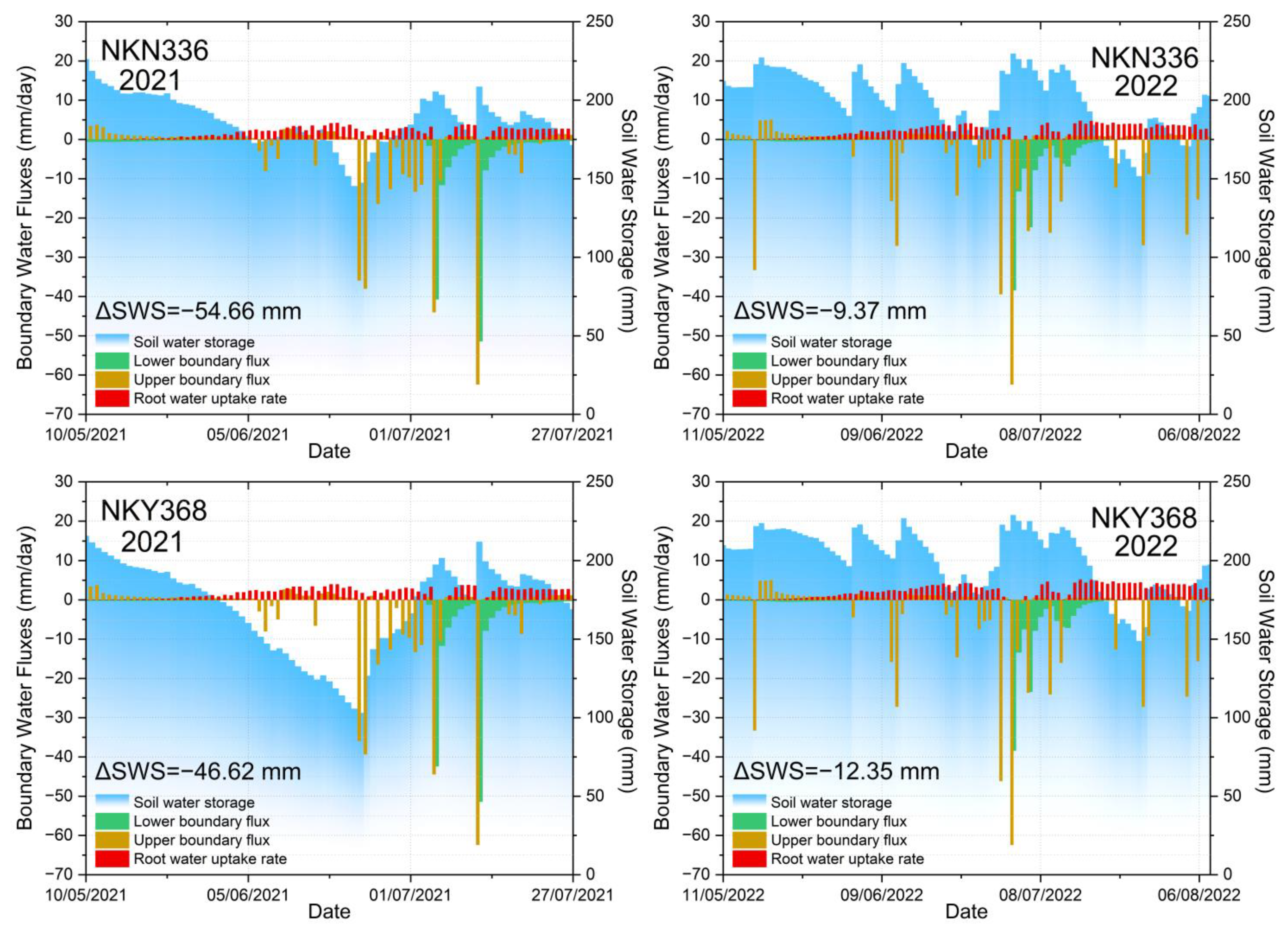
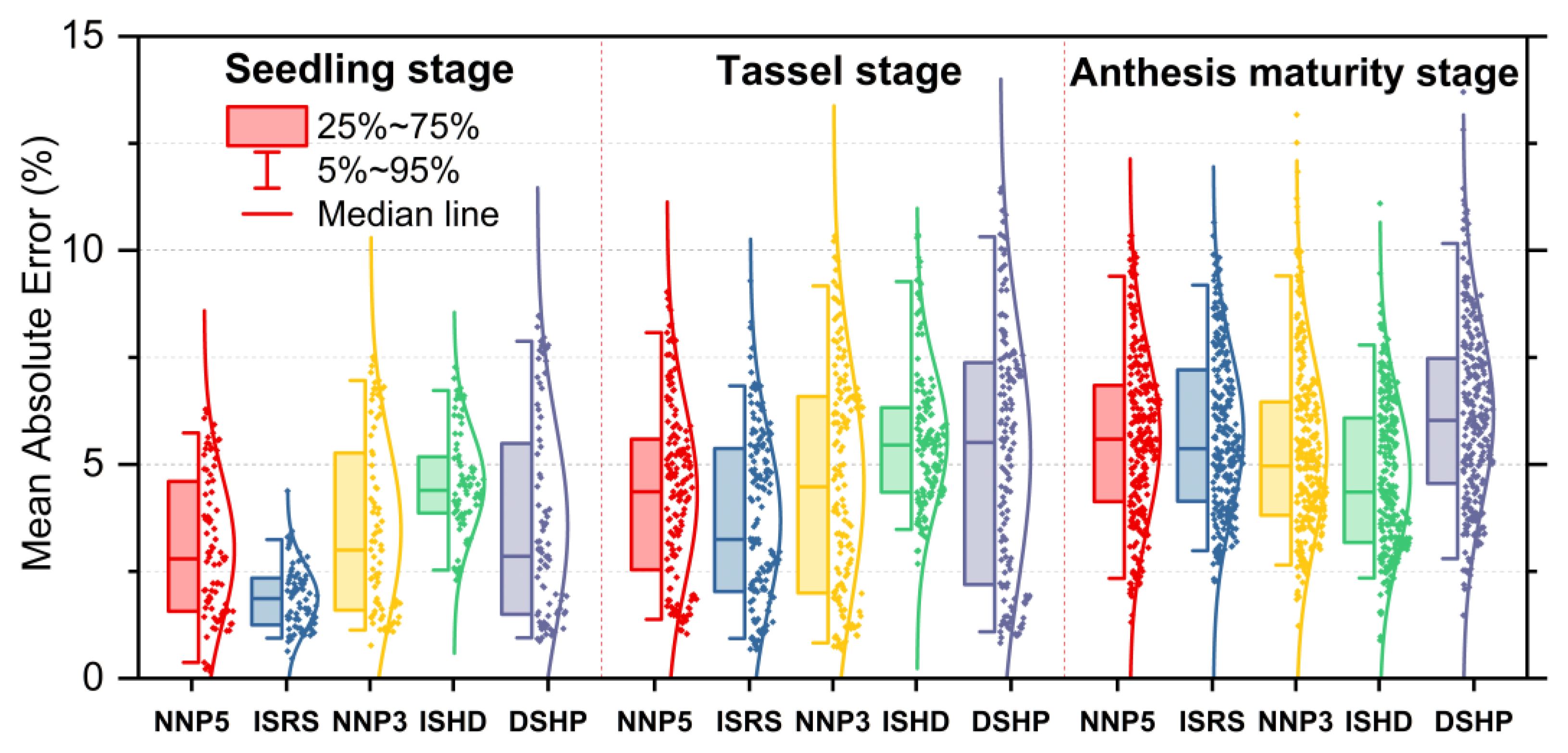
In this study, to evaluate the feasibility of using remote sensing data to optimize hydrodynamic soil parameters in the Hydrus-1D model, five types of soil hydrodynamic parameter acquisition methods were designed for a comparative evaluation from three parameter acquisition categories: parameters based on soil type default (DSHP), parameters based on soil mechanical composition prediction (NNP3 and NNP5), and parameters based on inverse solutions of historical data (ISHD and ISRS). Two crops of spring maize were planted in 2021 and 2022 at the Tongzhou base at the Maize Research Institute, Beijing Academy of Agricultural and Forestry Sciences, Beijing, China. Meteorological, soil, and crop data were collected during the maize-growing season. The boundary flux characteristics of the model simulation results were analyzed, and the accuracy differences in the five parameter acquisition methods were compared from three perspectives: overall root zone, growth stage, and soil depth. The results showed that (1) evapotranspiration was the main method for soil water depletion in the root zone of maize; the total actual evapotranspiration accounted for 68.26 and 69.43% of the total precipitation in 2021 and 2022, respectively, of which the root water uptake accounted for approximately 62.64% of the total actual evapotranspiration. (2) The accuracy of the SWC simulations in the root zone for different approaches were all acceptable in the following order: NNP5 (RMSE = 5.47%) > ISRS (RMSE = 5.48%) > NNP3 (RMSE = 5.66%) > ISHD (RMSE = 5.68%) > DSHP (RMSE = 6.57%). The ISRS approach based on remote sensing data achieved almost the best performance while effectively reducing the workload and cost. (3) The accuracy of the SWC simulation for different growth stages was ranked as follows: seedling stage (MAE = 3.29%) > tassel stage (MAE = 4.68%) > anthesis maturity stage (MAE = 5.52%). (4) The SWC errors simulated by all methods tended to decrease with increasing soil depth, whereas the ISHD method, based on measured historical data, achieved the best performance at a depth of 60 cm (MAE = 2.8%). Additionally, the results of the Pearson correlation analysis between each indicator (meteorology, soil, and crop) and MAE showed that the daily order of maize after planting (DOY) had the highest correlation with the MAE (R = 0.42), reflecting the time-cumulative nature of the model simulation errors.

However, there are still some limitations to this study in terms of soil texture complexity, crop species, and model optimization. In future studies, we will continue to enrich the diversity of the soil and crop species coverage in planting plots to obtain more widely representative results. At the same time, we will further expand the evaluation range and combination mode of remote sensing data sources; for example, other studies [61] have pointed out that the GLDAS-2.1 reanalysis dataset released by NASA has a better SWC correlation than ERA5-Land in some arid regions of China. This can be used for the parameter inverse solution of the Hydrus-1D model. Additionally, [33] pointed out that the Feddes model in the Hydrus-1D model is deficient for the fine simulation of dynamic crop growth processes. Studies have been conducted to couple crop models, such as DSSAT [35] and AquaCrop [68], with the Hydrus-1D model to achieve more accurate SWC simulation via crop models for enhancing the simulation accuracy of water uptake and Tp in the root zone of crops. Improving model simulation accuracy is also an important area for future research.

References

1. Tanumihardjo, S.A.; McCulley, L.; Roh, R.; Lopez-Ridaura, S.; Palacios-Rojas, N.; Gunaratna, N.S. Maize Agro-Food Systems to Ensure Food and Nutrition Security in Reference to the Sustainable Development Goals. Glob. Food Secur. 2020, 25, 100327. [Google Scholar] [CrossRef]
2. China National Bureau of Statistics Information Disclosure of National Bureau of Statistics. Available online: http://www.stats.gov.cn/xxgk/jd/sjjd2020/202112/t20211206_1825067.html (accessed on 11 June 2022).
3. Adeyemi, O.; Grove, I.; Peets, S.; Domun, Y.; Norton, T. Dynamic Neural Network Modelling of Soil Moisture Content for Predictive Irrigation Scheduling. Sensors 2018, 18, 3408. [Google Scholar] [CrossRef] [PubMed] [Green Version]
4. Peichl, M.; Thober, S.; Meyer, V.; Samaniego, L. The Effect of Soil Moisture Anomalies on Maize Yield in Germany. Nat. Hazards Earth Syst. Sci. 2018, 18, 889–906. [Google Scholar] [CrossRef] [Green Version]
5. Togneri, R.; Felipe dos Santos, D.; Camponogara, G.; Nagano, H.; Custódio, G.; Prati, R.; Fernandes, S.; Kamienski, C. Soil Moisture Forecast for Smart Irrigation: The Primetime for Machine Learning. Expert Syst. Appl. 2022, 207, 117653. [Google Scholar] [CrossRef]
6. Li, L.; Li, X.; Zheng, X.; Li, X.; Jiang, T.; Ju, H.; Wan, X. The Effects of Declining Soil Moisture Levels on Suitable Maize Cultivation Areas in Northeast China. J. Hydrol. 2022, 608, 127636. [Google Scholar] [CrossRef]
7. Yu, J.; Zhang, X.; Xu, L.; Dong, J.; Zhangzhong, L. A Hybrid CNN-GRU Model for Predicting Soil Moisture in Maize Root Zone. Agric. Water Manag. 2021, 245, 106649. [Google Scholar] [CrossRef]
8. Yu, J.; Tang, S.; Zhangzhong, L.; Zheng, W.; Wang, L.; Wong, A.; Xu, L. A Deep Learning Approach for Multi-Depth Soil Water Content Prediction in Summer Maize Growth Period. IEEE Access 2020, 8, 199097–199110. [Google Scholar] [CrossRef]
9. Cai, Y.; Zheng, W.; Zhang, X.; Zhangzhong, L.; Xue, X. Research on Soil Moisture Prediction Model Based on Deep Learning. PLoS ONE 2019, 14, e0214508. [Google Scholar] [CrossRef]
10. Hateffard, F.; Dolati, P.; Heidari, A.; Zolfaghari, A.A. Assessing the Performance of Decision Tree and Neural Network Models in Mapping Soil Properties. J. Mt. Sci. 2019, 16, 1833–1847. [Google Scholar] [CrossRef]
11. Lu, J.; Lu, H. Enhanced Cd Transport in the Soil-Plant-Atmosphere Continuum (SPAC) System by Tobacco (Nicotiana tabacum L.). Chemosphere 2019, 225, 395–405. [Google Scholar] [CrossRef]
12. Šimůnek, J.; van Genuchten, M.T.; Šejna, M. Recent Developments and Applications of the HYDRUS Computer Software Packages. Vadose Zone J. 2016, 15, vzj2016.04.003. [Google Scholar] [CrossRef] [Green Version]
13. Steduto, P.; Hsiao, T.C.; Raes, D.; Fereres, E. AquaCrop—The FAO Crop Model to Simulate Yield Response to Water: I. Concepts and Underlying Principles. Agron. J. 2009, 101, 426–437. [Google Scholar] [CrossRef] [Green Version]
14. Ebrahimi-Mollabashi, E.; Huth, N.I.; Holzwoth, D.P.; Ordóñez, R.A.; Hatfield, J.L.; Huber, I.; Castellano, M.J.; Archontoulis, S.V. Enhancing APSIM to Simulate Excessive Moisture Effects on Root Growth. Field Crops Res. 2019, 236, 58–67. [Google Scholar] [CrossRef]
15. Wang, Z.; Ye, L.; Jiang, J.; Fan, Y.; Zhang, X. Review of Application of EPIC Crop Growth Model. Ecol. Model. 2022, 467, 109952. [Google Scholar] [CrossRef]
16. Asada, K.; Eguchi, S.; Ikeba, M.; Kato, T.; Yada, S.; Nakajima, Y.; Itahashi, S. Modeling Nitrogen Leaching from Andosols Amended with Different Composted Manures Using LEACHM. Nutr. Cycl. Agroecosyst. 2018, 110, 307–326. [Google Scholar] [CrossRef]
17. Aguilera, H.; Moreno, L.; Wesseling, J.G.; Jiménez-Hernández, M.E.; Castaño, S. Soil Moisture Prediction to Support Management in Semiarid Wetlands during Drying Episodes. Catena 2016, 147, 709–724. [Google Scholar] [CrossRef]
18. Arshad Awan, Z.; Khaliq, T.; Masood Akhtar, M.; Imran, A.; Irfan, M.; Jarrar Ahmed, M.; Ahmad, A. Building Climate-Resilient Cotton Production System for Changing Climate Scenarios Using the DSSAT Model. Sustainability 2021, 13, 10495. [Google Scholar] [CrossRef]
19. Šimunek, J.; van Genuchten, M.T.; Šejna, M. HYDRUS: Model Use, Calibration, and Validation. Trans. ASABE 2012, 55, 1263. [Google Scholar] [CrossRef] [Green Version]
20. Tafteh, A.; Sepaskhah, A.R. Application of HYDRUS-1D Model for Simulating Water and Nitrate Leaching from Continuous and Alternate Furrow Irrigated Rapeseed and Maize Fields. Agric. Water Manag. 2012, 113, 19–29. [Google Scholar] [CrossRef]
21. Er-Raki, S.; Ezzahar, J.; Merlin, O.; Amazirh, A.; Hssaine, B.A.; Kharrou, M.H.; Khabba, S.; Chehbouni, A. Performance of the HYDRUS-1D Model for Water Balance Components Assessment of Irrigated Winter Wheat under Different Water Managements in Semi-Arid Region of Morocco. Agric. Water Manag. 2021, 244, 106546. [Google Scholar] [CrossRef]
22. Ventrella, D.; Castellini, M.; Di Prima, S.; Garofalo, P.; Lassabatère, L. Assessment of the Physically-Based Hydrus-1D Model for Simulating the Water Fluxes of a Mediterranean Cropping System. Water 2019, 11, 1657. [Google Scholar] [CrossRef] [Green Version]
23. Tu, A.; Xie, S.; Mo, M.; Song, Y.; Li, Y. Water Budget Components Estimation for a Mature Citrus Orchard of Southern China Based on HYDRUS-1D Model. Agric. Water Manag. 2021, 243, 106426. [Google Scholar] [CrossRef]
24. Haj-Amor, Z.; Bouri, S. Use of HYDRUS-1D–GIS Tool for Evaluating Effects of Climate Changes on Soil Salinization and Irrigation Management. Arch. Agron. Soil Sci. 2020, 66, 193–207. [Google Scholar] [CrossRef]
25. Lena, B.P.; Bondesan, L.; Pinheiro, E.A.R.; Ortiz, B.V.; Morata, G.T.; Kumar, H. Determination of Irrigation Scheduling Thresholds Based on HYDRUS-1D Simulations of Field Capacity for Multilayered Agronomic Soils in Alabama, USA. Agric. Water Manag. 2022, 259, 107234. [Google Scholar] [CrossRef]
26. Wang, X.; Li, Y.; Chen, X.; Wang, H.; Li, L.; Yao, N.; Liu, D.L.; Biswas, A.; Sun, S. Projection of the Climate Change Effects on Soil Water Dynamics of Summer Maize Grown in Water Repellent Soils Using APSIM and HYDRUS-1D Models. Comput. Electron. Agric. 2021, 185, 106142. [Google Scholar] [CrossRef]
27. Yinglan, A.; Wang, G.; Hu, P.; Lai, X.; Xue, B.; Fang, Q. Root-Zone Soil Moisture Estimation Based on Remote Sensing Data and Deep Learning. Environ. Res. 2022, 212, 113278. [Google Scholar] [CrossRef]
28. Mahmood, A.; Farhadi, L.; Heidary, P. A Framework for Coupled Estimation of Evapotranspiration and Recharge Flux by Assimilating Remotely Sensed Land Surface Temperature and Soil Moisture Observation. In Proceedings of the 2021 IEEE International Geoscience and Remote Sensing Symposium IGARSS, Brussels, Belgium, 11–16 July 2021; pp. 6455–6457. [Google Scholar]
29. Laluet, P.; Guerra, L.E.O.; Gaspar, V.A.; Rivalland, V.; Simonneaux, V.; Bustillo, V.; Bellvert, J.; Villar, J.M.; Merlin, O. Estimating the Drainage of Irrigated Areas: A Combined Crop Water Balance Modeling and Remote Sensing Approach. In Proceedings of the Copernicus Meetings, Montpellier, France, 29 May–3 June 2022. [Google Scholar]
30. Kocian, L.; Mohanty, B. Evaluating the Presence of Preferential Flow Using Machine Learning Algorithms and Remote Sensing Data. AGU Fall Meet. Abstr. 2021, 2021, H35P-1218. [Google Scholar]
31. Carsel, R.F.; Parrish, R.S. Developing Joint Probability Distributions of Soil Water Retention Characteristics. Water Resour. Res. 1988, 24, 755–769. [Google Scholar] [CrossRef] [Green Version]
32. Hopmans, J.W.; Bristow, K.L. Current Capabilities and Future Needs of Root Water and Nutrient Uptake Modeling. In Advances in Agronomy; Sparks, D.L., Ed.; Academic Press: Cambridge, MA, USA, 2002; Volume 77, pp. 103–183. [Google Scholar]
33. Zhu, W.; Li, H.; Qu, H.; Wang, Y.; Misselbrook, T.; Li, X.; Jiang, R. Water Stress in Maize Production in the Drylands of the Loess Plateau. Vadose Zone J. 2018, 17, 180117. [Google Scholar] [CrossRef] [Green Version]
34. Javadi, A.; Shayannejad, M.; Ebrahimian, H.; Ghorbani-Dashtaki, S. Simulation Modeling of Border Irrigation Performance under Different Soil Texture Classes and Land Uses. Model. Earth Syst. Environ. 2022, 8, 1135–1144. [Google Scholar] [CrossRef]
35. Shelia, V.; Šimůnek, J.; Boote, K.; Hoogenbooom, G. Coupling DSSAT and HYDRUS-1D for Simulations of Soil Water Dynamics in the Soil-Plant-Atmosphere System. J. Hydrol. Hydromech. 2018, 66, 232–245. [Google Scholar] [CrossRef]
36. Colliander, A.; Reichle, R.; Crow, W.; Cosh, M.; Chen, F.; Chan, S.; Das, N.N.; Bindlish, R.; Chaubell, J.; Kim, S.; et al. Validation of Soil Moisture Data Products From the NASA SMAP Mission. IEEE J. Sel. Top. Appl. Earth Obs. Remote Sens. 2022, 15, 364–392. [Google Scholar] [CrossRef]
37. Wang, X.; Lü, H.; Crow, W.T.; Zhu, Y.; Wang, Q.; Su, J.; Zheng, J.; Gou, Q. Assessment of SMOS and SMAP Soil Moisture Products against New Estimates Combining Physical Model, a Statistical Model, and in-Situ Observations: A Case Study over the Huai River Basin, China. J. Hydrol. 2021, 598, 126468. [Google Scholar] [CrossRef]
38. Colliander, A.; Jackson, T.J.; Bindlish, R.; Chan, S.; Das, N.; Kim, S.B.; Cosh, M.H.; Dunbar, R.S.; Dang, L.; Pashaian, L.; et al. Validation of SMAP Surface Soil Moisture Products with Core Validation Sites. Remote Sens. Environ. 2017, 191, 215–231. [Google Scholar] [CrossRef]
39. Nadeem, M.U.; Ghanim, A.A.J.; Anjum, M.N.; Shangguan, D.; Rasool, G.; Irfan, M.; Niazi, U.M.; Hassan, S. Multiscale Ground Validation of Satellite and Reanalysis Precipitation Products over Diverse Climatic and Topographic Conditions. Remote Sens. 2022, 14, 4680. [Google Scholar] [CrossRef]
40. Muñoz Sabater, J. ERA5-Land Hourly Data from 1981 to Present. Copernic. Clim. Chang. Serv. C3S Clim. Data Store CDS 2019, 10. [Google Scholar] [CrossRef]
41. Gorelick, N.; Hancher, M.; Dixon, M.; Ilyushchenko, S.; Thau, D.; Moore, R. Google Earth Engine: Planetary-Scale Geospatial Analysis for Everyone. Remote Sens. Environ. 2017, 202, 18–27. [Google Scholar] [CrossRef]
42. Richards, L.A. Capillary Conduction of Liquids through Porous Mediums. Physics 1931, 1, 318–333. [Google Scholar] [CrossRef]
43. van Genuchten, M.T. A Closed-Form Equation for Predicting the Hydraulic Conductivity of Unsaturated Soils. Soil Sci. Soc. Am. J. 1980, 44, 892–898. [Google Scholar] [CrossRef] [Green Version]
44. Allen, R.G.; Pereira, L.S.; Raes, D.; Smith, M. Crop Evapotranspiration. Guidelines for Computing Crop Water Requirements. FAO Irrig. Drain. Pap. FAO 1998, 300, D05109. [Google Scholar]
45. Belmans, C.; Wesseling, J.G.; Feddes, R.A. Simulation Model of the Water Balance of a Cropped Soil: SWATRE. J. Hydrol. 1983, 63, 271–286. [Google Scholar] [CrossRef]
46. Wu, Y.; Huang, M. Analysis of Influential Factors for Maize Root Water Uptake Based on Hydrus-1D Model. Trans. Chin. Soc. Agric. Eng. 2011, 27, 66–73. [Google Scholar]
47. Feddes, R.A. Simulation of Field Water Use and Crop Yield. In Simulation of Plant Growth and Crop Production; Pudoc: Wageningen, The Netherlands, 1982; pp. 194–209. [Google Scholar]
48. Wesseling, J.G.; Elbers, J.A.; Kabat, P.; Van den Broek, B.J. SWATRE: Instructions for Input; Internal Note; Winand Staring Centre: Wageningen, The Netherlands, 1991. [Google Scholar]
49. Schaap, M.G.; Leij, F.J.; van Genuchten, M.T. Rosetta: A Computer Program for Estimating Soil Hydraulic Parameters with Hierarchical Pedotransfer Functions. J. Hydrol. 2001, 251, 163–176. [Google Scholar] [CrossRef]
50. Šimůnek, J.; Hopmans, J.W. 1.7 Parameter Optimization and Nonlinear Fitting. In Methods of Soil Analysis; John Wiley & Sons, Ltd.: Hoboken, NJ, USA, 2002; pp. 139–157. ISBN 978-0-89118-893-3. [Google Scholar]
51. Chen, S.; Arrouays, D.; Leatitia Mulder, V.; Poggio, L.; Minasny, B.; Roudier, P.; Libohova, Z.; Lagacherie, P.; Shi, Z.; Hannam, J.; et al. Digital Mapping of GlobalSoilMap Soil Properties at a Broad Scale: A Review. Geoderma 2022, 409, 115567. [Google Scholar] [CrossRef]
52. Nachtergaele, F.O.; Spaargaren, O.; Deckers, J.A.; Ahrens, B. New Developments in Soil Classification: World Reference Base for Soil Resources. Geoderma 2000, 96, 345–357. [Google Scholar] [CrossRef]
53. García-Gaines, R.A.; Frankenstein, S. USCS and the USDA Soil Classification System: Development of a Mapping Scheme; U.S. Army Engineer Research and Development Center, Cold Regions Research and Engineering Laboratory: Hanover, NH, USA, 2015.
54. Gao, Y.; Zhang, M.; Wang, Z.; Zhang, Y. Yield Sustainability of Winter Wheat under Three Limited-Irrigation Schemes Based on a 28-Year Field Experiment. Crop J. 2022. [Google Scholar] [CrossRef]
55. Ma, X.Y.; Zhou, G.S. Method of Determining the Maximum Leaf Area Index of Spring Maize and Its Application. Acta Ecol. Sin. 2013, 33, 2596–2603. [Google Scholar]
56. Wang, X.L. How to Use the Logistic Equation Reasonably in the Simulation of Dry Matter Accumulation of Crops. Chin. J. Agrometeorol. 1986, 8, 14–19. [Google Scholar]
57. Myneni, R.; Knyazikhin, Y.; Park, T. MODIS/Terra+Aqua Leaf Area Index/FPAR 4-Day L4 Global 500m SIN Grid V061 [Data Set]; NASA EOSDIS Land Processes DAAC: Sioux Falls, SD, USA, 2015. [Google Scholar]
58. Chaoming, D.; Pengnian, W.; Ling, Y.; Yuhua, L.; Xiaokang, G.; Tongchao, W. Modelling the Effect of Tillage on Soil Water Dynamics in Corn Field. Guangai Paishui Xuebao 2020, 39, 24–31. [Google Scholar]
59. Noshadi, M.; Fahandej-Saadi, S.; Sepaskhah, A.R. Application of SALTMED and HYDRUS-1D Models for Simulations of Soil Water Content and Soil Salinity in Controlled Groundwater Depth. J. Arid Land 2020, 12, 447–461. [Google Scholar] [CrossRef]
60. Muñoz-Sabater, J.; Dutra, E.; Agustí-Panareda, A.; Albergel, C.; Arduini, G.; Balsamo, G.; Boussetta, S.; Choulga, M.; Harrigan, S.; Hersbach, H.; et al. ERA5-Land: A State-of-the-Art Global Reanalysis Dataset for Land Applications. Earth Syst. Sci. Data 2021, 13, 4349–4383. [Google Scholar] [CrossRef]
61. Wu, Z.; Feng, H.; He, H.; Zhou, J.; Zhang, Y. Evaluation of Soil Moisture Climatology and Anomaly Components Derived From ERA5-Land and GLDAS-2.1 in China. Water Resour. Manag. 2021, 35, 629–643. [Google Scholar] [CrossRef]
62. Pelosi, A.; Chirico, G.B. Regional Assessment of Daily Reference Evapotranspiration: Can Ground Observations Be Replaced by Blending ERA5-Land Meteorological Reanalysis and CM-SAF Satellite-Based Radiation Data? Agric. Water Manag. 2021, 258, 107169. [Google Scholar] [CrossRef]
63. Campos-Taberner, M.; Moreno-Martínez, Á.; García-Haro, F.J.; Camps-Valls, G.; Robinson, N.P.; Kattge, J.; Running, S.W. Global Estimation of Biophysical Variables from Google Earth Engine Platform. Remote Sens. 2018, 10, 1167. [Google Scholar] [CrossRef] [Green Version]
64. Jebli, I.; Belouadha, F.-Z.; Kabbaj, M.I.; Tilioua, A. Prediction of Solar Energy Guided by Pearson Correlation Using Machine Learning. Energy 2021, 224, 120109. [Google Scholar] [CrossRef]
65. Yu, J.; Zheng, W.; Xu, L.; Meng, F.; Li, J.; Zhangzhong, L. TPE-CatBoost: An Adaptive Model for Soil Moisture Spatial Estimation in the Main Maize-Producing Areas of China with Multiple Environment Covariates. J. Hydrol. 2022, 613, 128465. [Google Scholar] [CrossRef]
66. Alun, L.; Weizhong, Y.; Juan, L. Spatial Analysis Methods and Application of Regional Soil Moisture. Chin. Agric. Sci. Bull. 2012, 2012, 60. [Google Scholar]
67. Klute, A.; Dirksen, C. Hydraulic Conductivity and Diffusivity: Laboratory Methods. In Methods of Soil Analysis; John Wiley & Sons, Ltd.: Hoboken, NJ, USA, 1986; pp. 687–734. ISBN 978-0-89118-864-3. [Google Scholar]
68. Kanda, E.K.; Senzanje, A.; Mabhaudhi, T. Coupling Hydrus 2D/3D and AquaCrop Models for Simulation of Water Use in Cowpea (Vigna Unguiculata (L.) Walp). In Proceedings of the Sustaining Tomorrow; Ting, D.S.-K., Vasel-Be-Hagh, A., Eds.; Springer International Publishing: Cham, Switzerland, 2021; pp. 53–63. [Google Scholar]
Figure 1. The technical route of this study.
Remotesensing 14 06079 g001
Figure 2. Overview of the Hydrus-1D model soil moisture simulation process.
Remotesensing 14 06079 g002
Figure 3. Different methods for obtaining soil hydraulic parameters for the Hydrus-1D model.
Remotesensing 14 06079 g003
Figure 4. Overview map of experiment area and sensor deployments.
Remotesensing 14 06079 g004
Figure 5. Processes and statistical characteristics of changes in the soil water content (SWC) in the root zone profiles of different plots.
Remotesensing 14 06079 g005aRemotesensing 14 06079 g005b
Figure 6. Trends in potential evapotranspiration rate and leaf area index (LAI) coefficient.
Remotesensing 14 06079 g006
Figure 7. Changes in boundary fluxes and soil water storage in different plots.
Remotesensing 14 06079 g007aRemotesensing 14 06079 g007b
Figure 8. Simulation effect of parameters for the ISHD inverse solution method on JKT608.
Remotesensing 14 06079 g008
Figure 9. Variation characteristics of the model simulation error in the time dimension.
Remotesensing 14 06079 g009
Figure 10. Characteristics of the model simulation errors at different growth stages.
Remotesensing 14 06079 g010
Figure 11. Correlation coefficients between the model simulated MAE and multiple indicators. * Indicates significant correlation at the 0.05 level.
Remotesensing 14 06079 g011
Figure 12. Distribution of the simulation errors for the Hydrus-1D model at different soil depths.
Remotesensing 14 06079 g012aRemotesensing 14 06079 g012b