
Impacts of Extreme Temperature and Precipitation on Crops during the Growing Season in South Asia

 , , ,
, , ,
Abstract
:1. Introduction
2. Materials and Methods
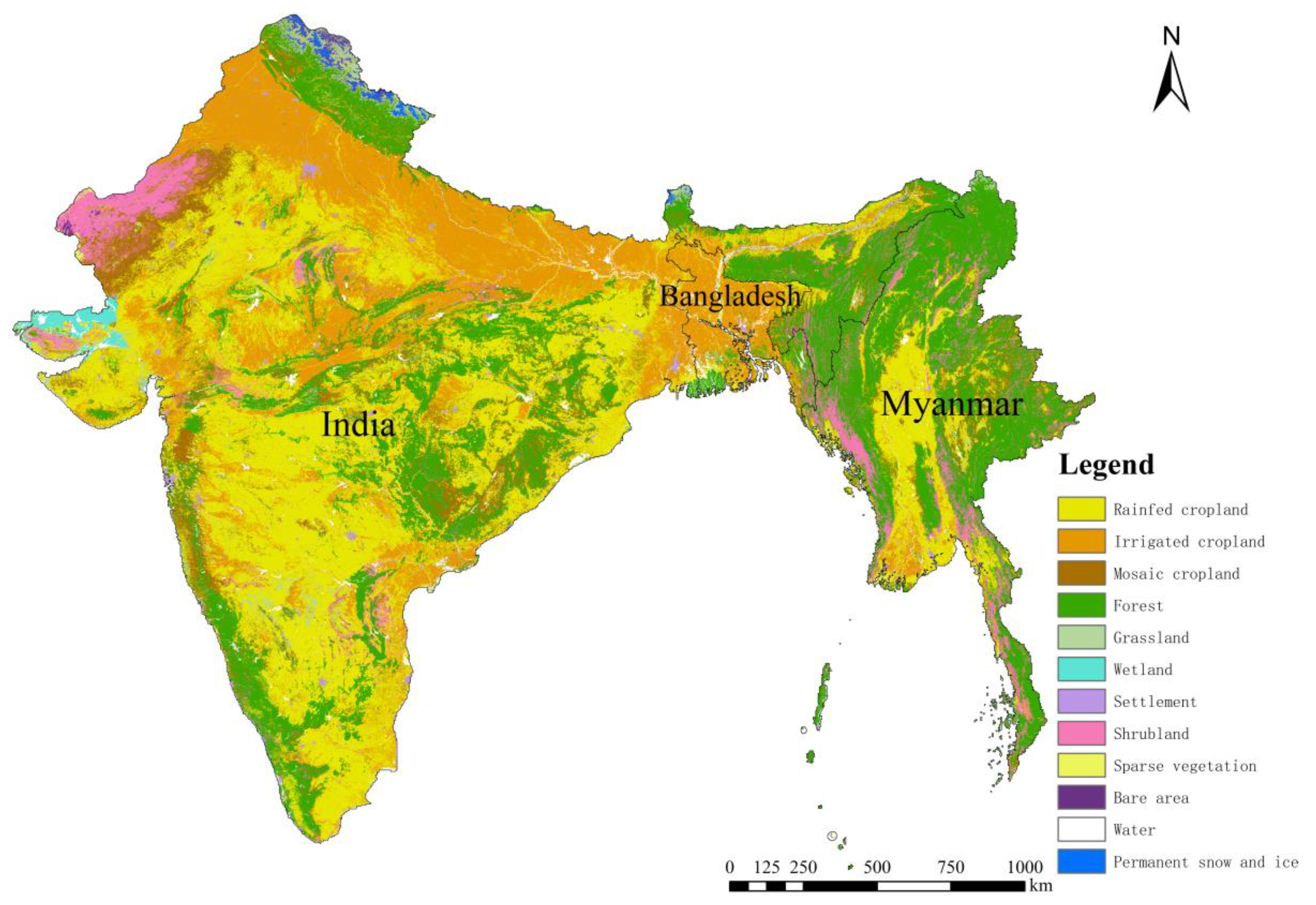
2.1. Study Area
2.2. Data
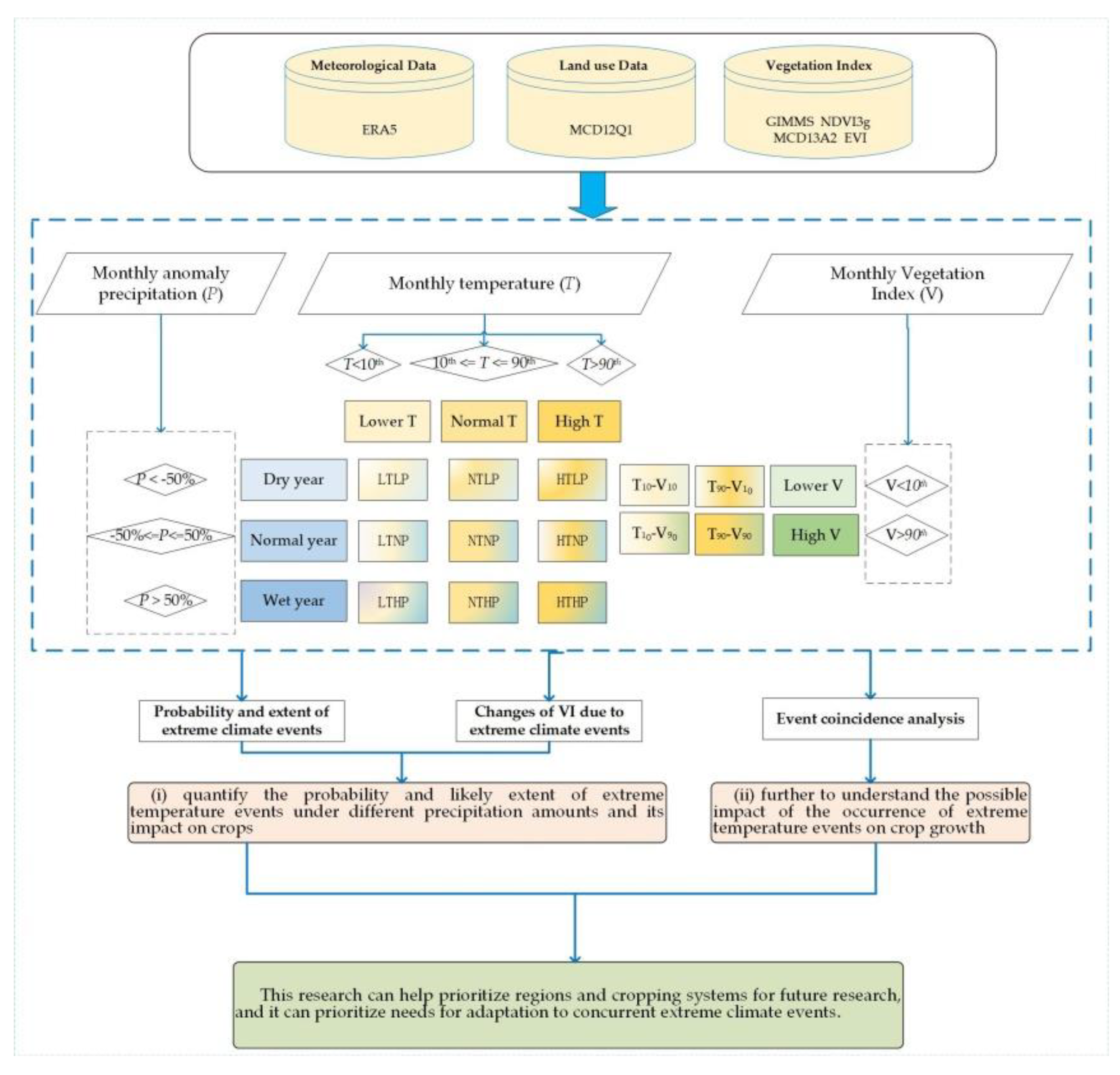
2.3. Methods
2.3.1. Frequency and Extent of Climate Extreme Events
- HTHP: T > 90th and P > 50%,
- HTNP: T > 90th and −50% ≤ P ≤ 50%,
- HTLP: T > 90th and P < −50%,
- NTHP: 10th ≤ T ≤ 90th and P > 50%,
- NTNP: 10th ≤ T ≤ 90th and −50% ≤ P ≤ 50%,
- NTLP: 10th ≤ T ≤ 90th and P < −50%,
- LTHP: T < 10th and P > 50%,
- LTNP: T < 10th and −50% ≤ P ≤ 50%,
- LTLP: T < 10th and P < −50%.
2.3.2. Measuring Influence of Extreme Climate Events on Crop Growth
2.3.3. Event Coincidence Rate between Extreme Temperature and Extreme EVI
- (i)
- Both 2 m temperature and EVI are greater than their respective empirical 90% quantiles (in the following referred to as T90–V90)
- (ii)
- Both 2 m temperature and EVI are lower than their 10% quantile (T10–V10)
- (iii)
- 2 m temperature is lower than its 10% and EVI is greater than its 90% quantile (T10–V90)
- (iv)
- 2 m temperature is greater than its 90% and EVI is lower than its 10% quantile (T90–V10)
3. Results
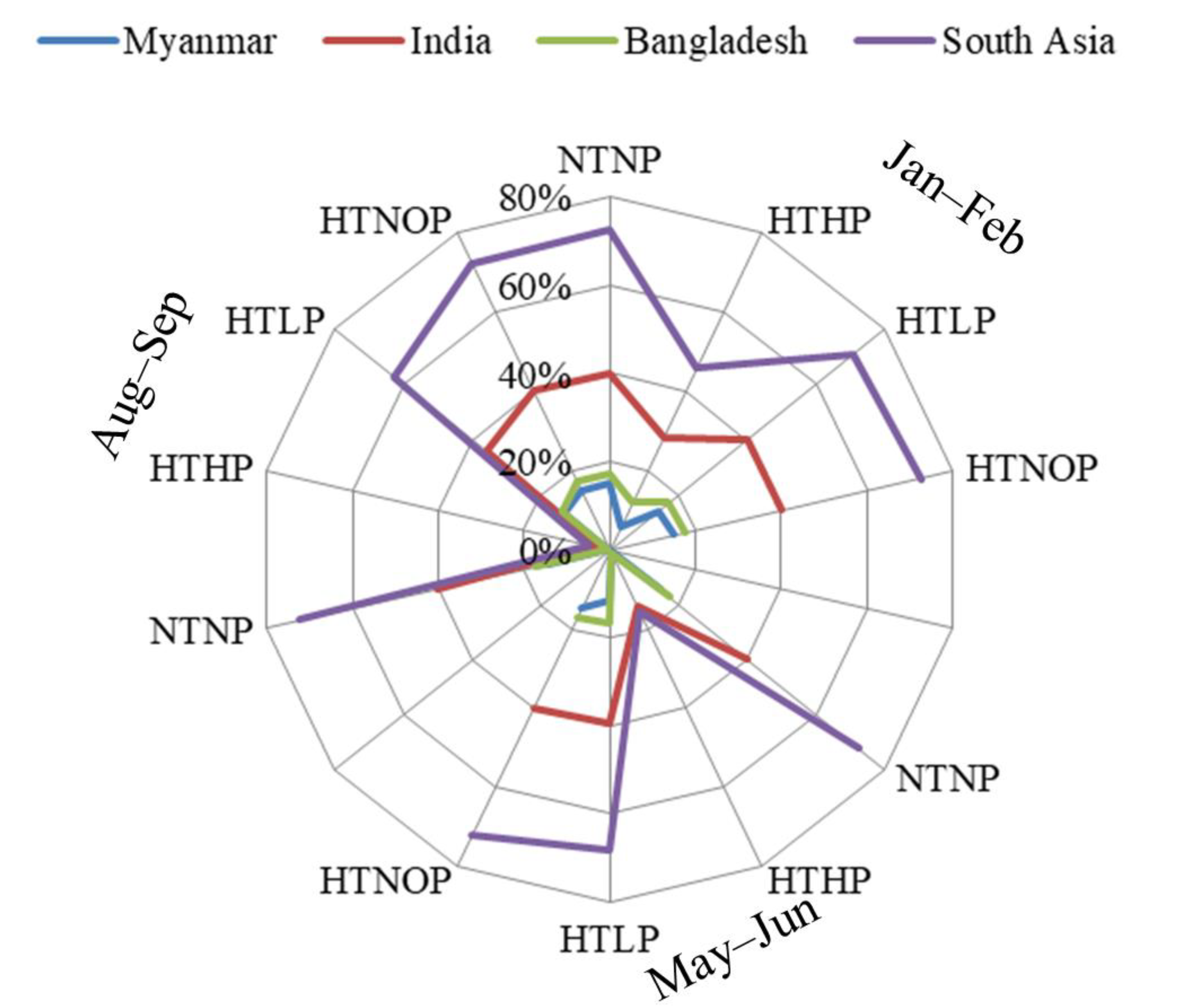
3.1. Probabilities of Extreme Climate Events
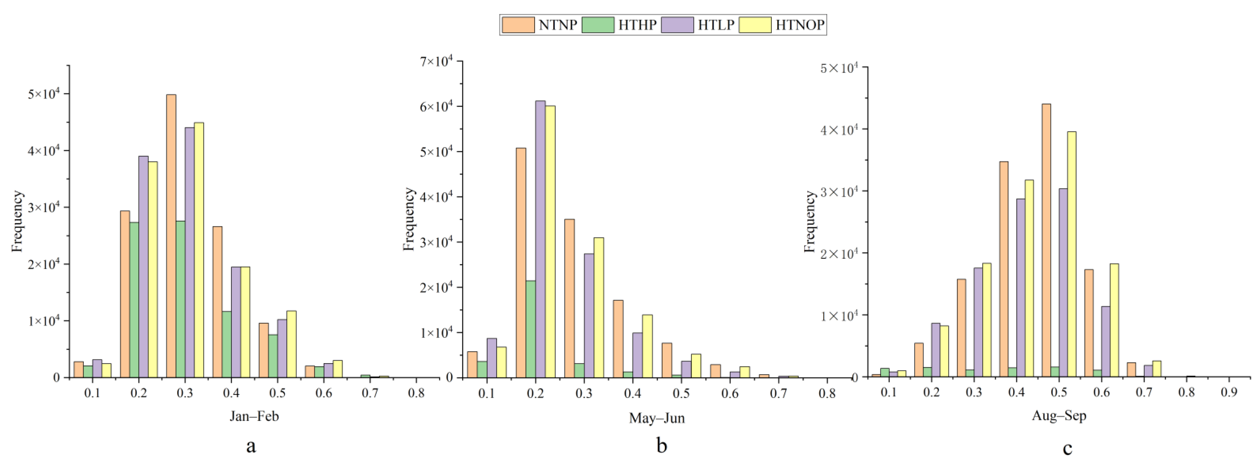
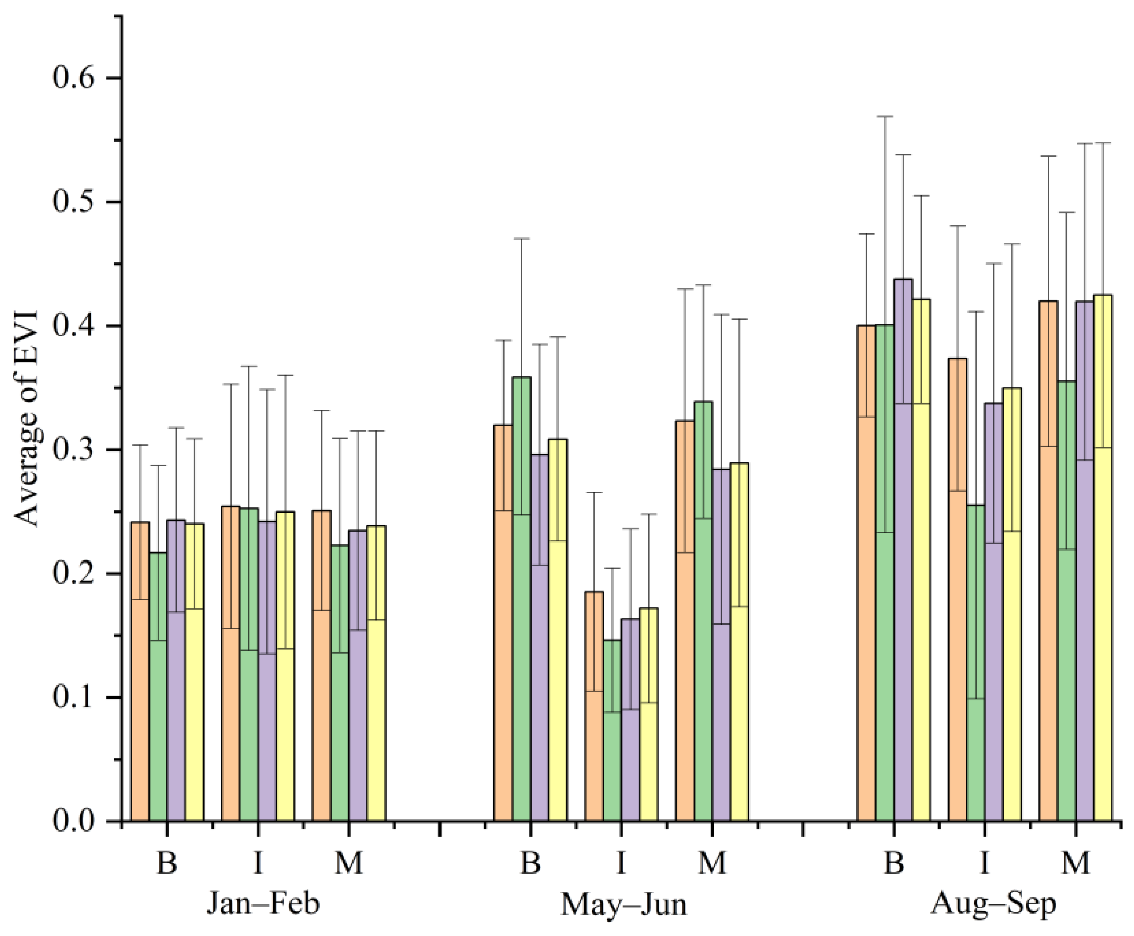
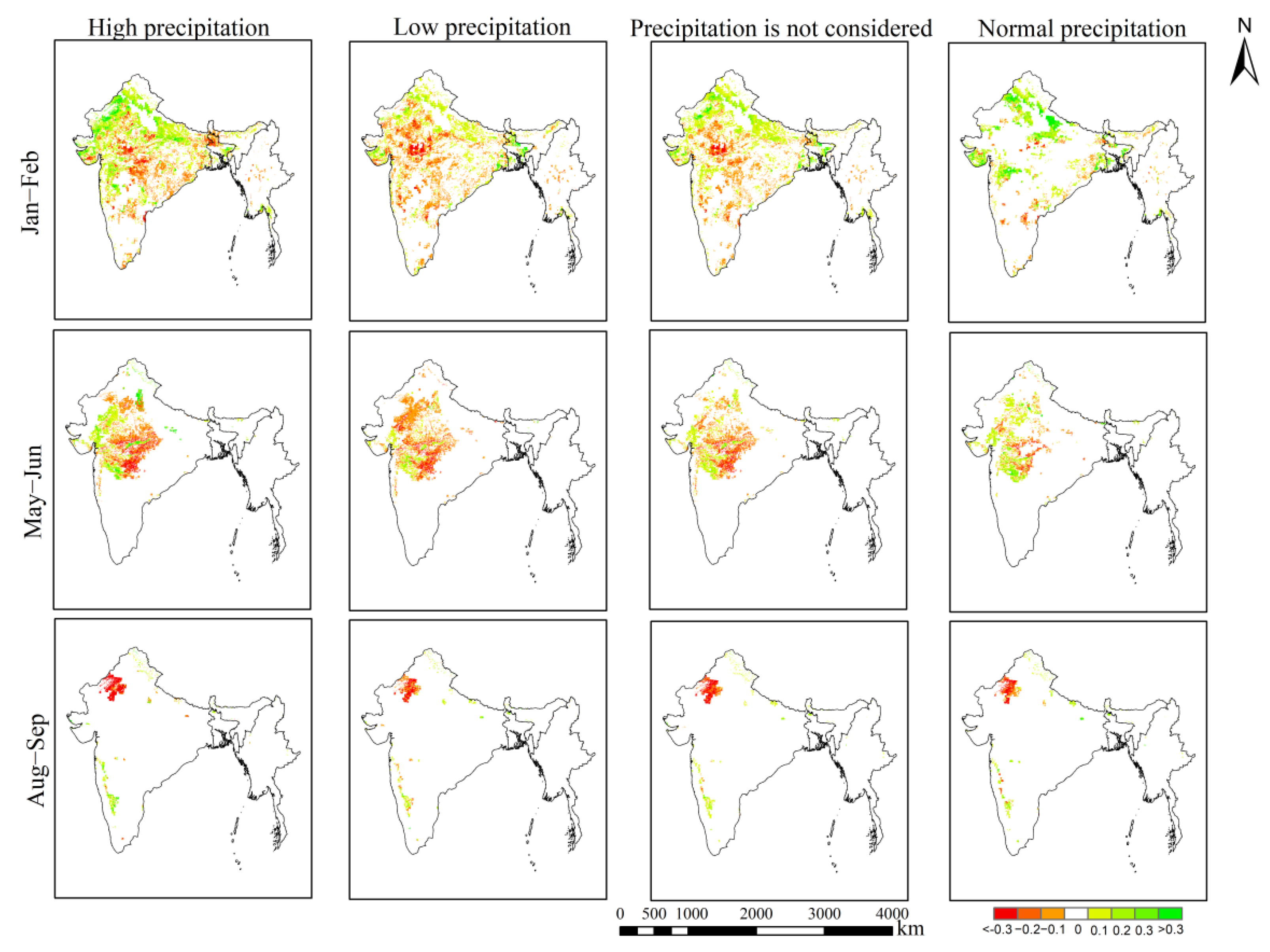
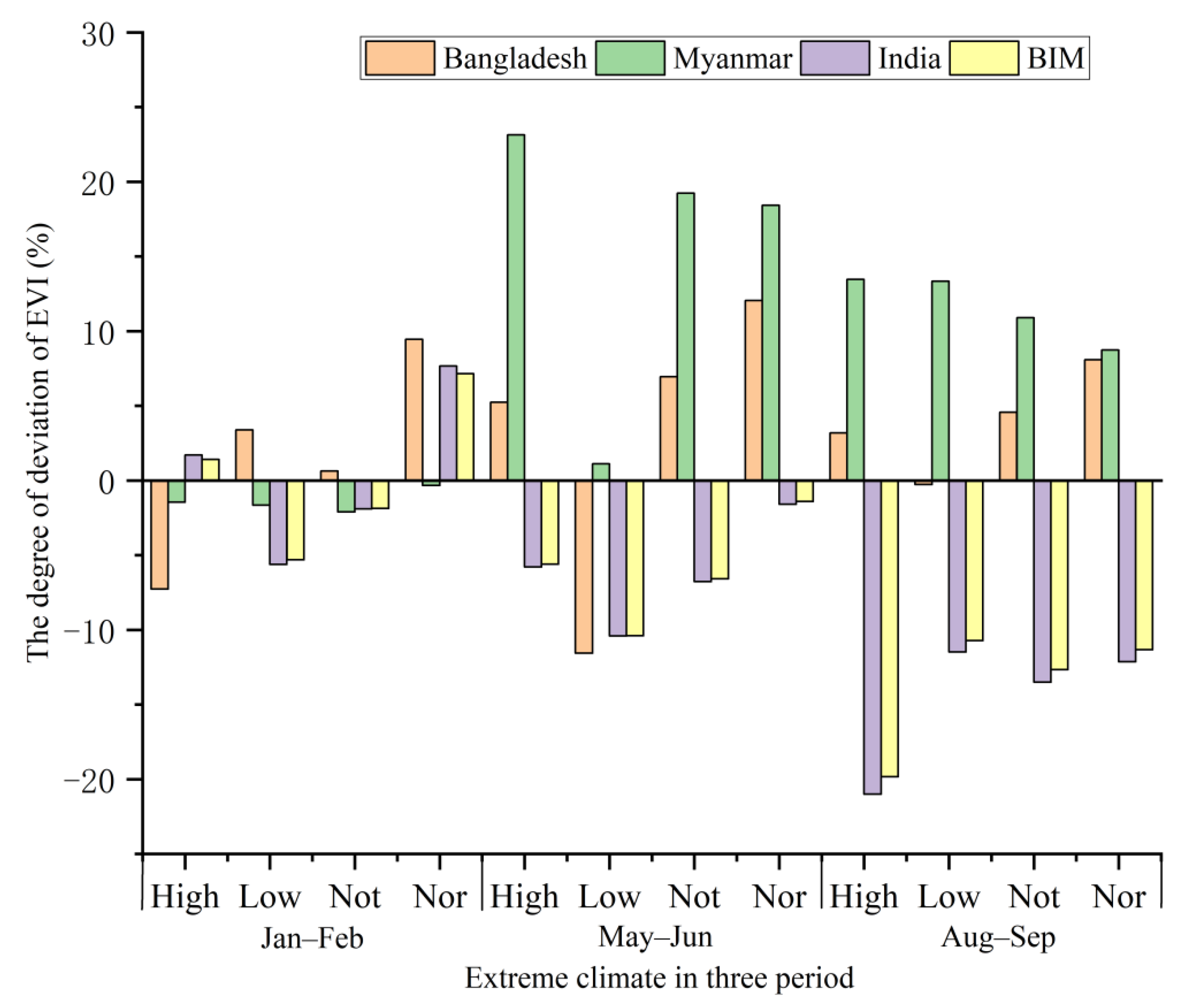
3.2. Changes of EVI Due to Extreme Climate Events
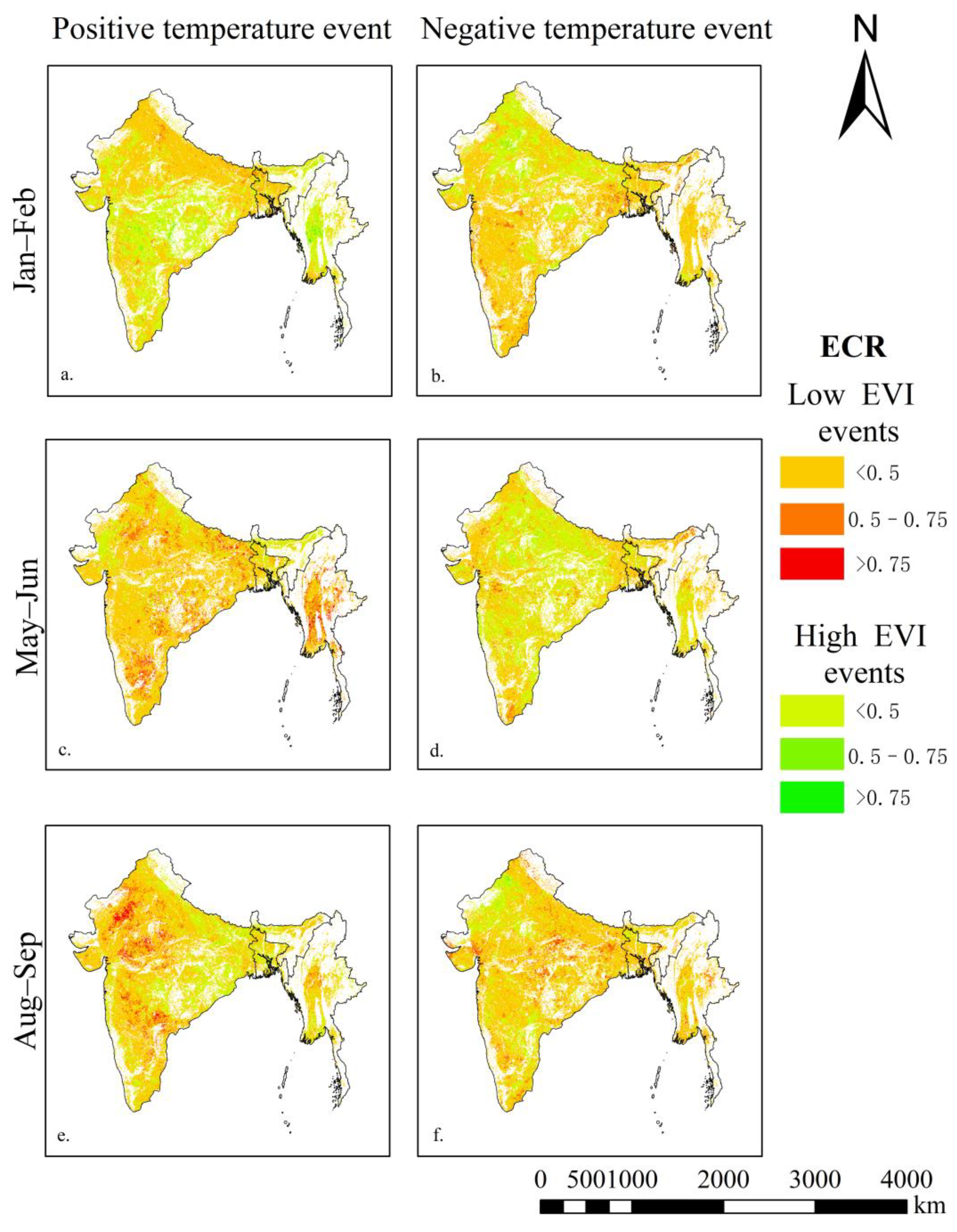
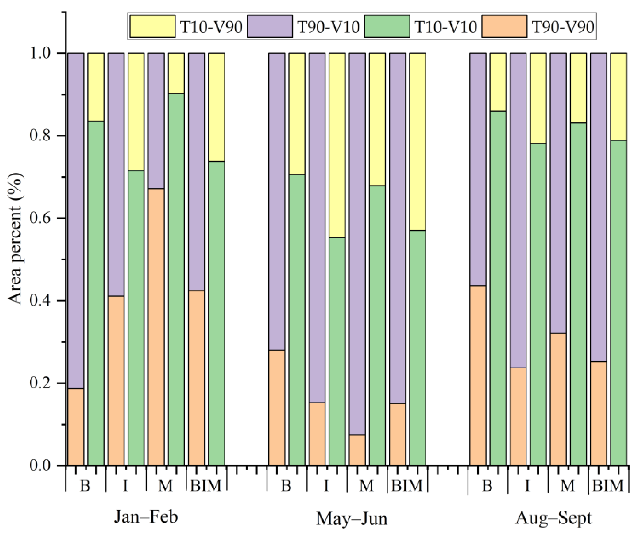
3.3. Event Coincidence Analysis
4. Discussion
4.1. Extreme Climate Events under Global Warming
4.2. The Mechanism of Crop Yield Reduction Caused by Extreme Climate
4.3. Similarities and Differences in Vegetation Index
4.4. Adapting Measures to Climate Change
5. Conclusions
Supplementary Materials
Author Contributions
Funding
Data Availability Statement
Acknowledgments
Conflicts of Interest
Appendix A
References
- Lai, L.W. The relationship between extreme weather events and crop losses in central Taiwan. Theor. Appl. Climatol. 2018, 134, 107–119. [Google Scholar] [CrossRef]
- Lesk, C.; Rowhani, P.; Ramankutty, N. Influence of extreme weather disasters on global crop production. Nature 2016, 529, 84–87. [Google Scholar] [CrossRef] [Green Version]
- Regan, P.M.; Kim, H.; Maiden, E. Climate change, adaptation, and agricultural output. Reg. Environ. Chang. 2018, 19, 113–123. [Google Scholar] [CrossRef]
- Trenberth, K.E. Changes in precipitation with climate change. Clim. Res. 2011, 47, 123–138. [Google Scholar] [CrossRef] [Green Version]
- Wassmann, R.; Jagadish, S.V.K.; Sumfleth, K.; Pathak, H.; Howell, G.; Ismail, A.; Serraj, R.; Redona, E.; Singh, R.K.; Heuer, S. Chapter 3 Regional Vulnerability of Climate Change Impacts on Asian Rice Production and Scope for Adaptation. Adv. Agron. 2009, 102, 91–133. [Google Scholar]
- Rummukainen, M. Changes in climate and weather extremes in the 21st century. Wiley Interdiscip. Rev. Clim. Chang. 2012, 3, 115–129. [Google Scholar] [CrossRef]
- Yin, J.; Gentine, P.; Zhou, S.; Sullivan, S.C.; Wang, R.; Zhang, Y.; Guo, S. Large increase in global storm runoff extremes driven by climate and anthropogenic changes. Nat. Commun. 2018, 9, 4389. [Google Scholar] [CrossRef] [Green Version]
- Mojid, M.A. Climate change-induced challenges to sustainable development in Bangladesh. IOP Conf. Ser. Earth Environ. Sci. 2020, 423, 012001. [Google Scholar] [CrossRef]
- Mishra, A.; Singh, R.; Raghuwanshi, N.S.; CHATTERJEE, C.; Froebrich, J. Spatial variability of climate change impacts on yield of rice and wheat in the Indian Ganga Basin. Sci. Total Environ. 2013, 468, S132–S138. [Google Scholar] [CrossRef]
- Rohini, P.; Rajeevan, M.; Mukhopadhay, P. Future projections of heat waves over India from CMIP5 models. Clim. Dyn. 2019, 53, 975–988. [Google Scholar] [CrossRef]
- Sattar, A.; Srivastava, R.C. Modelling climate smart rice-wheat production system in the middle Gangetic plains of India. Theor. Appl. Climatol. 2021, 144, 77–91. [Google Scholar] [CrossRef]
- Sillmann, J.; Kharin, V.V.; Zwiers, F.W.; Zhang, X.; Bronaugh, D. Climate extremes indices in the CMIP5 multimodel ensemble: Part 2. Future climate projections. J. Geophys. Res. Atmos. 2013, 118, 2473–2493. [Google Scholar] [CrossRef]
- Gu, H.; Wang, G.; Yu, Z.; Mei, R. Assessing future climate changes and extreme indicators in east and south Asia using the RegCM4 regional climate model. Clim. Chang. 2012, 114, 301–317. [Google Scholar] [CrossRef]
- Brown, P.T.; Caldeira, K. Greater future global warming inferred from Earth’s recent energy budget. Nature 2017, 552, 45–50. [Google Scholar] [CrossRef] [PubMed]
- Huang, J.; Zhang, X.; Zhang, Q.; Lin, Y.; Hao, M.; Luo, Y.; Zhao, Z.; Yao, Y.; Chen, X.; Wang, L.; et al. Recently amplified arctic warming has contributed to a continual global warming trend. Nat. Clim. Chang. 2017, 7, 875–879. [Google Scholar] [CrossRef]
- Swami, D.; Dave, P.; Parthasarathy, D. Analysis of temperature variability and extremes with respect to crop threshold temperature for Maharashtra, India. Theor. Appl. Climatol. 2021, 144, 861–872. [Google Scholar] [CrossRef]
- Chowdhury, M.A.; Zzaman, R.U.; Tarin, N.J.; Hossain, M.J. Spatial variability of climatic hazards in Bangladesh. Nat. Hazards 2021, 110, 2329–2351. [Google Scholar] [CrossRef]
- Sein, Z.M.M.; Zhi, X.; Ogou, F.K.; Nooni, I.K.; Lim Kam Sian, K.T.C.; Gnitou, G.T. Spatio-Temporal Analysis of Drought Variability in Myanmar Based on the Standardized Precipitation Evapotranspiration Index (SPEI) and Its Impact on Crop Production. Agronomy 2021, 11, 1691. [Google Scholar] [CrossRef]
- Zhu, X.; Troy, T.J. Agriculturally Relevant Climate Extremes and Their Trends in the World’s Major Growing Regions. Earth’s Future 2018, 6, 656–672. [Google Scholar] [CrossRef]
- Dash, B.K.; Rafiuddin, M.; Khanam, F.; Islam, M.N. Characteristics of meteorological drought in Bangladesh. Nat. Hazards 2012, 64, 1461–1474. [Google Scholar] [CrossRef]
- Hoarau, K.; Bernard, J.; Chalonge, L. Intense tropical cyclone activities in the northern Indian Ocean. Int. J. Climatol. 2012, 32, 1935–1945. [Google Scholar] [CrossRef]
- Khudri, M.M.; Bagmar, M.S.H.; Redwan, A.M. Characterisation of spatio-temporal trend in temperature extremes for environmental decision making in Bangladesh. Int. J. Glob. Warm. 2019, 19, 364–381. [Google Scholar] [CrossRef]
- Swain, M.; Sinha, P.; Mohanty, U.C.; Pattnaik, S. Dominant large-scale parameters responsible for diverse extreme rainfall events over vulnerable Odisha state in India. Clim. Dyn. 2019, 53, 6629–6644. [Google Scholar] [CrossRef]
- Sikka, A.K.; Rao, B.B.; Rao, V.U.M. Agricultural disaster management and contingency planning to meet the challenges of extreme weather events. Mausam 2016, 67, 155–168. [Google Scholar] [CrossRef]
- Aleshina, M.A.; Semenov, V.A.; Chernokulsky, A.V. A link between surface air temperature and extreme precipitation over Russia from station and reanalysis data. Environ. Res. Lett. 2021, 16, 105004. [Google Scholar] [CrossRef]
- Chan, S.C.; Kendon, E.J.; Roberts, N.M.; Fowler, H.J.; Blenkinsop, S. Downturn in scaling of UK extreme rainfall with temperature for future hottest days. Nat. Geosci. 2016, 9, 24–28. [Google Scholar] [CrossRef] [Green Version]
- Lenderink, G.; Barbero, R.; Westra, S.; Fowler, H.J. Reply to comments on “Temperature-extreme precipitation scaling: A two-way causality?”. Int. J. Climatol. 2018, 38, 4664–4666. [Google Scholar] [CrossRef] [Green Version]
- Hernandez, M.J.; Montes, F.; Ruiz, F.; Lopez, G.; Pita, P. The effect of vapour pressure deficit on stomatal conductance, sap pH and leaf-specific hydraulic conductance in Eucalyptus globulus clones grown under two watering regimes. Ann. Bot. 2016, 117, 1063–1071. [Google Scholar] [CrossRef] [Green Version]
- Huybers, P.; Holbrook, N.M.; Siebert, S.; Ray, D.K.; Butler, E.E.; Rhines, A.; Mueller, N.D. Global Relationships between Cropland Intensification and Summer Temperature Extremes over the Last 50 Years. J. Clim. 2017, 30, 7505–7528. [Google Scholar]
- Lee, S.; Bae, Y.S.; Kim, H.S. The Study and Analysis of Extreme Weather in Seoul. Seoul Stud. 2011, 12, 1–17. [Google Scholar]
- Min, S.-K.; Son, S.-W.; Seo, K.-H.; Kug, J.-S.; An, S.-I.; Choi, Y.-S.; Jeong, J.-H.; Kim, B.-M.; Kim, J.-W.; Kim, Y.-H.; et al. Changes in weather and climate extremes over Korea and possible causes: A review. Asia-Pac. J. Atmos. Sci. 2015, 51, 103–121. [Google Scholar] [CrossRef]
- van der Wiel, K.; Selten, F.M.; Bintanja, R.; Blackport, R.; Screen, J.A. Ensemble climate-impact modelling: Extreme impacts from moderate meteorological conditions. Environ. Res. Lett. 2020, 15, 034050. [Google Scholar] [CrossRef]
- Zeng, F.W.; Collatz, G.J.; Pinzon, J.E.; Ivanoff, A. Evaluating and Quantifying the Climate-Driven Interannual Variability in Global Inventory Modeling and Mapping Studies (GIMMS) Normalized Difference Vegetation Index (NDVI3g) at Global Scales. Remote Sens. 2013, 5, 3918–3950. [Google Scholar] [CrossRef]
- Wang, J.B.; Dong, J.W.; Liu, J.Y.; Huang, M.; Li, G.C.; Running, S.W.; Smith, W.K.; Harris, W.; Saigusa, N.; Kondo, H.; et al. Comparison of Gross Primary Productivity Derived from GIMMS NDVI3g, GIMMS, and MODIS in Southeast Asia. Remote Sens. 2014, 6, 2108–2133. [Google Scholar] [CrossRef] [Green Version]
- Tiedemann, J.L. Fenología y productividad primaria neta aérea de sistemas pastoriles de Panicum maximun en el dpto. Moreno, Santiago del Estero, Argentina, derivada del NDVI MODIS. Ecol. Apl. 2015, 14, 27–39. [Google Scholar] [CrossRef] [Green Version]
- Valverde-Arias, O.; Garrido, A.; Valencia, J.L.; Maria Tarquis, A. Using geographical information system to generate a drought risk map for rice cultivation: Case study in Babahoyo canton (Ecuador). Biosyst. Eng. 2018, 168, 26–41. [Google Scholar] [CrossRef]
- Vannoppen, A.; Gobin, A.; Kotova, L.; Top, S.; De Cruz, L.; Viksna, A.; Aniskevich, S.; Bobylev, L.; Buntemeyer, L.; Caluwaerts, S.; et al. Wheat Yield Estimation from NDVI and Regional Climate Models in Latvia. Remote Sens. 2020, 12, 2206. [Google Scholar] [CrossRef]
- Xu, X.; Piao, S.; Wang, X.; Chen, A.; Ciais, P.; Myneni, R.B. Spatio-temporal patterns of the area experiencing negative vegetation growth anomalies in China over the last three decades. Environ. Res. Lett. 2012, 7, 035701. [Google Scholar] [CrossRef]
- Huete, A.; Justice, C.; Liu, H. Development of vegetation and soil indices for MODIS-EOS. Remote Sens. Environ. 1994, 49, 224–234. [Google Scholar] [CrossRef]
- Stoy, P.C.; Mauder, M.; Foken, T.; Marcolla, B.; Boegh, E.; Ibrom, A.; Arain, M.A.; Arneth, A.; Aurela, M.; Bernhofer, C.; et al. A data-driven analysis of energy balance closure across FLUXNET research sites: The role of landscape scale heterogeneity. Agric. For. Meteorol. 2013, 171, 137–152. [Google Scholar] [CrossRef] [Green Version]
- Wardlow, B.D.; Egbert, S.L.; Kastens, J.H. Analysis of time-series MODIS 250 m vegetation index data for crop classification in the US Central Great Plains. Remote Sens. Environ. 2007, 108, 290–310. [Google Scholar] [CrossRef] [Green Version]
- Xiao, X.; Hollinger, D.; Aber, J.; Goltz, M.; Davidson, E.A.; Zhang, Q.; Moore, B. Satellite-based modeling of gross primary production in an evergreen needleleaf forest. Remote Sens. Environ. 2004, 89, 519–534. [Google Scholar] [CrossRef]
- Lyapustin, A.; Alexander, M.J.; Ott, L.; Molod, A.; Holben, B.; Susskind, J.; Wang, Y. Observation of mountain lee waves with MODIS NIR column water vapor. Geophys. Res. Lett. 2014, 41, 710–716. [Google Scholar] [CrossRef]
- Didan, K.; Munoz, A.B.; Solano, R.; Huete, A. MODIS Vegetation Index User’s Guide (MOD13 Series); Vegetation Index and Phenology Lab, University of Arizona: Tucson, AZ, USA, 2015. [Google Scholar]
- Mishra, V. Long-term (1870–2018) drought reconstruction in context of surface water security in India. J. Hydrol. 2020, 580, 124228. [Google Scholar] [CrossRef]
- Mishra, V.; Tiwari, A.D.; Aadhar, S.; Shah, R.; Xiao, M.; Pai, D.S.; Lettenmaier, D. Drought and Famine in India, 1870–2016. Geophys. Res. Lett. 2019, 46, 2075–2083. [Google Scholar] [CrossRef]
- Thomas, T.; Nayak, P.C.; Ghosh, N.C. Irrigation planning for sustainable rain-fed agriculture in the drought-prone Bundelkhand region of Madhya Pradesh, India. J. Water Clim. Chang. 2014, 5, 408–426. [Google Scholar] [CrossRef]
- Biradar, C.M.; Xiao, X. Quantifying the area and spatial distribution of double- and triple-cropping croplands in India with multi-temporal MODIS imagery in 2005. Int. J. Remote Sens. 2011, 32, 367–386. [Google Scholar] [CrossRef]
- Hossain, M.S.; Qian, L.; Arshad, M.; Shahid, S.; Fahad, S.; Akhter, J. Climate change and crop farming in Bangladesh: An analysis of economic impacts. Int. J. Clim. Chang. Strateg. Manag. 2019, 11, 424–440. [Google Scholar] [CrossRef] [Green Version]
- Gumma, M.K.; Thenkabail, P.S.; Deevi, K.C.; Mohammed, I.A.; Teluguntla, P.; Oliphant, A.; Xiong, J.; Aye, T.; Whitbread, A.M. Mapping cropland fallow areas in myanmar to scale up sustainable intensification of pulse crops in the farming system. GIScience Remote Sens. 2018, 55, 926–949. [Google Scholar] [CrossRef]
- Huete, A.; Didan, K.; Miura, T.; Rodriguez, E.P.; Gao, X.; Ferreira, L.G. Overview of the radiometric and biophysical performance of the MODIS vegetation indices. Remote Sens. Environ. 2002, 83, 195–213. [Google Scholar] [CrossRef]
- Zhengxing, W.; Chuang, L.; Alfredo, H. From AVHRR-NDVI to MODIS-EVI: Advances in vegetation index research. Acta Ecol. Sin. 2003, 23, 979–987. [Google Scholar]
- Tucker, C.J.; Pinzon, J.E.; Brown, M.E.; Slayback, D.A.; Pak, E.W.; Mahoney, R.; Vermote, E.F.; El Saleous, N. An extended AVHRR 8-km NDVI dataset compatible with MODIS and SPOT vegetation NDVI data. Int. J. Remote Sens. 2005, 26, 4485–4498. [Google Scholar] [CrossRef]
- Pinzon, J.E.; Tucker, C.J. A Non-Stationary 1981–2012 AVHRR NDVI3g Time Series. Remote Sens. 2014, 6, 6929–6960. [Google Scholar] [CrossRef] [Green Version]
- Hersbach, H.; Bell, B.; Berrisford, P.; Hirahara, S.; Horányi, A.; Muñoz-Sabater, J.; Nicolas, J.; Peubey, C.; Radu, R.; Schepers, D. The ERA5 global reanalysis. Q. J. R. Meteorol. Soc. 2020, 146, 1999–2049. [Google Scholar] [CrossRef]
- Copernicus Climate Change Service. ERA5: Fifth generation of ECMWF atmospheric reanalyses of the global climate. Copernic. Clim. Chang. Serv. Clim. Data Store (CDS) 2017, 15, 2020. [Google Scholar]
- Bontemps, S.; Defourny, P.; Radoux, J.; Van Bogaert, E.; Lamarche, C.; Achard, F.; Mayaux, P.; Boettcher, M.; Brockmann, C.; Kirches, G. Consistent global land cover maps for climate modelling communities: Current achievements of the ESA’s land cover CCI. In Proceedings of the ESA Living Planet Symposium, Edinburgh, UK, 13 December 2013; pp. 9–13. [Google Scholar]
- Li, W.; MacBean, N.; Ciais, P.; Defourny, P.; Lamarche, C.; Bontemps, S.; Houghton, R.A.; Peng, S. Gross and net land cover changes in the main plant functional types derived from the annual ESA CCI land cover maps (1992–2015). Earth Syst. Sci. Data 2018, 10, 219–234. [Google Scholar] [CrossRef] [Green Version]
- Al-Nassar, A.R.; Jansa, A.; Sangrà, P.; Alarcon, M.; Jansa, A. Cut-off low systems over Iraq: Contribution to annual precipitation and synoptic analysis of extreme events. Int. J. Climatol. 2019, 40, 908–926. [Google Scholar] [CrossRef]
- Baumbach, L.; Siegmund, J.F.; Mittermeier, M.; Donner, R.V. Impacts of temperature extremes on European vegetation during the growing season. Biogeosciences 2017, 14, 4891–4903. [Google Scholar] [CrossRef] [Green Version]
- Donges, J.F.; Schleussner, C.F.; Siegmund, J.F.; Donner, R.V. Event coincidence analysis for quantifying statistical interrelationships between event time series. Eur. Phys. J. Spec. Top. 2016, 225, 471–487. [Google Scholar] [CrossRef] [Green Version]
- Odenweller, A.; Donner, R.V. Disentangling synchrony from serial dependency in paired-event time series. Phys. Rev. E 2020, 101, 052213. [Google Scholar] [CrossRef]
- Masson-Delmotte, V.; Zhai, P.; Pirani, A.; Connors, S.L.; Péan, C.; Berger, S.; Caud, N.; Chen, Y.; Goldfarb, L.; Gomis, M. Climate Change 2021: The Physical Science Basis. Contribution of Working Group I to the Sixth Assessment Report of the Intergovernmental Panel on Climate Change. 2021. Available online: https://www.ipcc.ch/report/ar6/wg1/ (accessed on 14 October 2022).
- Sedlmeier, K.; Feldmann, H.; Schädler, G. Compound summer temperature and precipitation extremes over central Europe. Theor. Appl. Climatol. 2017, 131, 1493–1501. [Google Scholar] [CrossRef]
- Gu, L.; Chen, J.; Yin, J.B.; Slater, L.J.; Wang, H.M.; Guo, Q.; Feng, M.Y.; Qin, H.; Zhao, T.T.G. Global Increases in Compound Flood-Hot Extreme Hazards Under Climate Warming. Geophys. Res. Lett. 2022, 49, e2022GL097726. [Google Scholar] [CrossRef]
- van der Velde, M.; Tubiello, F.N.; Vrieling, A.; Bouraoui, F. Impacts of extreme weather on wheat and maize in France: Evaluating regional crop simulations against observed data. Clim. Chang. 2012, 113, 751–765. [Google Scholar] [CrossRef] [Green Version]
- Hansen, J.; Sato, M.; Ruedy, R. Perception of climate change. Proc. Natl. Acad. Sci. USA 2012, 109, E2415–E2423. [Google Scholar] [CrossRef] [PubMed] [Green Version]
- Singh, V.; Goyal, M.K. Spatio-temporal heterogeneity and changes in extreme precipitation over eastern Himalayan catchments India. Stoch. Environ. Res. Risk Assess. 2017, 31, 2527–2546. [Google Scholar] [CrossRef]
- Vinnarasi, R.; Dhanya, C.T. Changing characteristics of extreme wet and dry spells of Indian monsoon rainfall. J. Geophys. Res.-Atmos. 2016, 121, 2146–2160. [Google Scholar] [CrossRef]
- Reshma, T.; Varikoden, H.; Babu, C.A. Observed Changes in Indian Summer Monsoon Rainfall at Different Intensity Bins during the Past 118 Years over Five Homogeneous Regions. Pure Appl. Geophys. 2021, 178, 3655–3672. [Google Scholar] [CrossRef]
- Sahu, R.T.; Verma, M.K.; Ahmad, I. Some non-uniformity patterns spread over the lower Mahanadi River Basin, India. Geocarto Int. 2021, 23, 1010–6049. [Google Scholar] [CrossRef]
- Zampieri, A.C.M.; Dentener, F.; Toreti, A. Wheat yield loss attributable to heat waves, drought and water excess at the global, national and subnational scales. Environ. Res. Lett. 2017, 12, 064008. [Google Scholar] [CrossRef]
- Prado, K.; Maurel, C. Regulation of leaf hydraulics: From molecular to whole plant levels. Front. Plant Sci. 2013, 4, 255. [Google Scholar] [CrossRef] [Green Version]
- Degife, A.W.; Zabel, F.; Mauser, W. Climate change impacts on potential maize yields in Gambella Region, Ethiopia. Reg. Environ. Chang. 2021, 21, 60. [Google Scholar] [CrossRef]
- Hao, Z.; Hao, F.; Singh, V.P.; Zhang, X. Changes in the severity of compound drought and hot extremes over global land areas. Environ. Res. Lett. 2018, 13, 124022. [Google Scholar] [CrossRef]
- Huo, Y.; Peltier, W.R. Dynamically Downscaled Climate Change Projections for the South Asian Monsoon: Mean and Extreme Precipitation Changes and Physics Parameterization Impacts. J. Clim. 2020, 33, 2311–2331. [Google Scholar] [CrossRef]
- Xu, Y.; Zhou, B.-T.; Wu, J.; Han, Z.-Y.; Zhang, Y.-X.; Wu, J. Asian climate change under 1.5–4 degrees C warming targets. Adv. Clim. Chang. Res. 2017, 8, 99–107. [Google Scholar] [CrossRef]
- Reddy, K.R.; Seghal, A.; Jumaa, S.; Bheemanahalli, R.; Kakar, N.; Redoña, E.D.; Wijewardana, C.; Alsajri, F.A.; Chastain, D.; Gao, W.; et al. Morpho-Physiological Characterization of Diverse Rice Genotypes for Seedling Stage High- and Low-Temperature Tolerance. Agronomy 2021, 11, 112. [Google Scholar] [CrossRef]
- Hasanuzzaman, M.; Nahar, K.; Alam, M.M.; Roychowdhury, R.; Fujita, M. Physiological, biochemical, and molecular mechanisms of heat stress tolerance in plants. Int. J. Mol. Sci. 2013, 14, 9643–9684. [Google Scholar] [CrossRef]
- Lesk, C.; Anderson, W. Decadal variability modulates trends in concurrent heat and drought over global croplands. Environ. Res. Lett. 2021, 16, 055024. [Google Scholar] [CrossRef]
- Lobell, D.B.; Hammer, G.L.; McLean, G.; Messina, C.; Roberts, M.J.; Schlenker, W. The critical role of extreme heat for maize production in the United States. Nat. Clim. Chang. 2013, 3, 497–501. [Google Scholar] [CrossRef]
- Tack, J.; Barkley, A.; Hendricks, N. Irrigation offsets wheat yield reductions from warming temperatures. Environ. Res. Lett. 2017, 12, 114027. [Google Scholar] [CrossRef]
- Tao, F.; Zhang, S.; Zhang, Z. Changes in rice disasters across China in recent decades and the meteorological and agronomic causes. Reg. Environ. Chang. 2012, 13, 743–759. [Google Scholar] [CrossRef]
- Timsina, J.; Jat, M.L.; Majumdar, K. Rice-maize systems of South Asia: Current status, future prospects and research priorities for nutrient management. Plant Soil 2010, 335, 65–82. [Google Scholar] [CrossRef]
- Li, Y.; Guan, K.; Peng, B.; Franz, T.E.; Wardlow, B.; Pan, M. Quantifying irrigation cooling benefits to maize yield in the US Midwest. Glob. Chang. Biol. 2020, 26, 3065–3078. [Google Scholar] [CrossRef] [PubMed]
- Luan, X.; Bommarco, R.; Scaini, A.; Vico, G. Combined heat and drought suppress rainfed maize and soybean yields and modify irrigation benefits in the USA. Environ. Res. Lett. 2021, 16, 064023. [Google Scholar] [CrossRef]
- Minoli, S.; Mueller, C.; Elliott, J.; Ruane, A.C.; Jaegermeyr, J.; Zabel, F.; Dury, M.; Folberth, C.; Francois, L.; Hank, T.; et al. Global Response Patterns of Major Rainfed Crops to Adaptation by Maintaining Current Growing Periods and Irrigation. Earths Future 2019, 7, 1464–1480. [Google Scholar] [CrossRef]
- Rao, A.; Chandran, M.A.S.; Bal, S.K.; Pramod, V.P.; Sandeep, V.M.; Manikandan, N.; Raju, B.M.K.; Prabhakar, M.; Islam, A.; Kumar, S.N.; et al. Evaluating area-specific adaptation strategies for rainfed maize under future climates of India. Sci. Total Environ. 2022, 836, 155511. [Google Scholar]
- Mishra, V.; Ambika, A.K.; Asoka, A.; Aadhar, S.; Buzan, J.; Kumar, R.; Huber, M. Moist heat stress extremes in India enhanced by irrigation. Nat. Geosci. 2020, 13, 722–728. [Google Scholar] [CrossRef]
- Jackson, N.D.; Konar, M.; Debaere, P.; Sheffield, J. Crop-specific exposure to extreme temperature and moisture for the globe for the last half century. Environ. Res. Lett. 2021, 16, 064006. [Google Scholar] [CrossRef]
- Babaeian, F.; Delavar, M.; Morid, S.; Srinivasan, R. Robust climate change adaptation pathways in agricultural water management. Agric. Water Manag. 2021, 252, 106904. [Google Scholar] [CrossRef]
- Duffy, C.; Pede, V.; Toth, G.; Kilcline, K.; O’Donoghue, C.; Ryan, M.; Spillane, C. Drivers of household and agricultural adaptation to climate change in Vietnam. Clim. Dev. 2020, 13, 242–255. [Google Scholar] [CrossRef]
- Harvey, R.J.; Chadwick, D.R.; Sánchez-Rodríguez, A.R.; Jones, D.L. Agroecosystem resilience in response to extreme winter flooding. Agric. Ecosyst. Environ. 2019, 279, 1–13. [Google Scholar] [CrossRef] [Green Version]
- Holzkämper, A.; Klein, T.; Seppelt, R.; Fuhrer, J. Assessing the propagation of uncertainties in multi-objective optimization for agro-ecosystem adaptation to climate change. Environ. Model. Softw. 2015, 66, 27–35. [Google Scholar] [CrossRef]
- Khanal, U.; Wilson, C.; Hoang, V.N.; Lee, B.L. Autonomous adaptations to climate change and rice productivity: A case study of the Tanahun district, Nepal. Clim. Dev. 2019, 11, 555–563. [Google Scholar] [CrossRef]
- Beacham, A.M.; Hand, P.; Barker, G.C.; Denby, K.J.; Teakle, G.R.; Walley, P.G.; Monaghan, J.M. Addressing the threat of climate change to agriculture requires improving crop resilience to short-term abiotic stress. Outlook Agric. 2018, 47, 270–276. [Google Scholar] [CrossRef]
- Kato, T.; Kimura, R.; Kamichika, M. Estimation of evapotranspiration, transpiration ratio and water-use efficiency from a sparse canopy using a compartment model. Agric. Water Manag. 2004, 65, 173–191. [Google Scholar] [CrossRef]
- Singh, N.P.; Anand, B.; Khan, M.A. Micro-level perception to climate change and adaptation issues: A prelude to mainstreaming climate adaptation into developmental landscape in India. Nat. Hazards 2018, 92, 1287–1304. [Google Scholar] [CrossRef]
- Skinner, C.B.; Poulsen, C.J.; Mankin, J.S. Amplification of heat extremes by plant CO2 physiological forcing. Nat. Commun. 2018, 9, 1094. [Google Scholar] [CrossRef]
- Alamgir, M.; Khan, N.; Shahid, S.; Yaseen, Z.M.; Dewan, A.; Hassan, Q.; Rasheed, B. Evaluating severity-area-frequency (SAF) of seasonal droughts in Bangladesh under climate change scenarios. Stoch. Environ. Res. Risk Assess. 2020, 34, 447–464. [Google Scholar] [CrossRef]
- Arreyndip, N.A. Identifying agricultural disaster risk zones for future climate actions. PLoS ONE 2021, 16, e0260430. [Google Scholar] [CrossRef]
- Islam, A.R.M.T.; Nabila, I.A.; Hasanuzzaman, M.; Rahman, M.B.; Elbeltagi, A.; Mallick, J.; Techato, K.; Pal, S.C.; Rahman, M.M. Variability of climate-induced rice yields in northwest Bangladesh using multiple statistical modeling. Theor. Appl. Climatol. 2022, 147, 1263–1276. [Google Scholar] [CrossRef]
- Islam, A.R.M.T.; Rahman, M.S.; Khatun, R.; Hu, Z. Spatiotemporal trends in the frequency of daily rainfall in Bangladesh during 1975–2017. Theor. Appl. Climatol. 2020, 141, 869–887. [Google Scholar] [CrossRef]
- Jha, R.; Mondal, A.; Devanand, A.; Roxy, M.K.; Ghosh, S. Limited influence of irrigation on pre-monsoon heat stress in the Indo-Gangetic Plain. Nat. Commun. 2022, 13, 4275. [Google Scholar] [CrossRef] [PubMed]
- Lacombe, G.; Chu Thai, H.; Smakhtin, V. Multi-year variability or unidirectional trends? Mapping long-term precipitation and temperature changes in continental Southeast Asia using PRECIS regional climate model. Clim. Chang. 2012, 113, 285–299. [Google Scholar] [CrossRef]
- Prodhan, F.A.; Zhang, J.; Sharma, T.P.P.; Nanzad, L.; Zhang, D.; Seka, A.M.; Ahmed, N.; Hasan, S.S.; Hoque, M.Z.; Mohana, H.P. Projection of future drought and its impact on simulated crop yield over South Asia using ensemble machine learning approach. Sci. Total Environ. 2022, 807, 151029. [Google Scholar] [CrossRef] [PubMed]


| Country | Crop | Variety | Jan. | Feb. | Mar. | Apr. | May | Jun. | Jul. | Aug. | Sep. | Oct. | Nov. | Dec. |
|---|---|---|---|---|---|---|---|---|---|---|---|---|---|---|
| Bangladesh | rice | Aus | sowing | growing | harvest | |||||||||
| kharif | harvest | sowing | growing | harvest | ||||||||||
| Rabi | sowing | growing | harvest | sowing | ||||||||||
| wheat | growing | harvest | sowing | |||||||||||
| India | rice | Aus | sowing | growing | harvest | |||||||||
| Kharif | sowing | growing | harvest | |||||||||||
| Rabi | growing | harvest | sowing | |||||||||||
| wheat | growing | harvest | sowing | |||||||||||
| Myanmar | rice | Aus | harvest | sowing | growing | harvest | ||||||||
| Rabi | growing | harvest | sowing | |||||||||||
| wheat | growing | harvest | sowing | |||||||||||
| Product | Range | Temporal Resolution | Spatial Resolution | Resampling | |
|---|---|---|---|---|---|
| NDVI | GIMMS NDVI3g | 1982–2015 | Monthly | 5000 m | Monthly 5000 m × 5000 m |
| EVI | MOD13C2 | 2000–2018 | Monthly | 5000 m | |
| Temperature and Precipitation | ERA5 | 1982–2018 | 8-days | 0.25° | |
| Land use | ESA CCI | 2020 | Year | 300 m |
| Probability (%) | Distribution Area (%) | |||||
|---|---|---|---|---|---|---|
| Jan–Feb | May–Jun | Aug–Sep | Jan–Feb | May–Jun | Aug–Sep | |
| LTLP | 4.56 | 0.44 | 0.61 | 92.14 | 13.02 | 14.50 |
| LTNP | 2.18 | 4.02 | 6.16 | 62.52 | 84.95 | 91.64 |
| LTHP | 3.56 | 5.84 | 3.52 | 84.63 | 86.78 | 93.38 |
| NTLP | 41.35 | 25.79 | 11.77 | 100.00 | 97.57 | 96.60 |
| NTNP | 19.23 | 37.87 | 57.66 | 100.00 | 100.00 | 100.00 |
| NTHP | 18.82 | 15.76 | 9.98 | 100.00 | 99.61 | 93.20 |
| HTLP | 6.81 | 7.19 | 4.19 | 99.01 | 97.11 | 85.52 |
| HTNP | 1.68 | 2.54 | 5.97 | 55.47 | 86.73 | 93.86 |
| HTHP | 1.80 | 0.57 | 0.13 | 67.16 | 25.75 | 5.41 |
| 2000–2018 | Grop | Sum | Mean | Variance | SS | df | MF | F | α | F Crit | |
|---|---|---|---|---|---|---|---|---|---|---|---|
| January–February | NTNP | 31,873.58 | 0.26 | 0.01 | Within groups | 9.16 | 3.00 | 3.05 | 292.58 | 0.00 | 2.60 |
| HTHP | 20,033.14 | 0.25 | 0.01 | ||||||||
| HTLP | 30,092.49 | 0.25 | 0.01 | Between groups | 4566.31 | 437,428.00 | 0.01 | ||||
| HTNOP | 31,191.08 | 0.26 | 0.01 | ||||||||
| May–June | NTNP | 28,007.44 | 0.23 | 0.01 | Within groups | 165.15 | 3.00 | 55.05 | 5211.33 | 0.00 | 2.60 |
| HTHP | 4777.05 | 0.16 | 0.01 | ||||||||
| HTLP | 22,283.32 | 0.20 | 0.01 | Between groups | 4040.82 | 382,534.00 | 0.01 | ||||
| HTNOP | 25,670.35 | 0.21 | 0.01 | ||||||||
| August–September | NTNP | 47,735.72 | 0.40 | 0.01 | Within groups | 95.39 | 3.00 | 31.80 | 2377.91 | 0.00 | 2.60 |
| HTHP | 2472.22 | 0.30 | 0.03 | ||||||||
| HTLP | 36,986.52 | 0.37 | 0.01 | Between groups | 4640.95 | 347,078.00 | 0.01 | ||||
| HTNOP | 46,522.06 | 0.39 | 0.01 |
| Significant Event Coincidence Rates (%) | Jan–Feb | May–Jun | Aug–Sep | |||||||||
|---|---|---|---|---|---|---|---|---|---|---|---|---|
| B | I | M | BIM | B | I | M | BIM | B | I | M | BIM | |
| T90–V90 | 5.10 | 13.80 | 27.00 | 14.52 | 8.76 | 4.60 | 2.89 | 4.57 | 14.49 | 7.39 | 10.08 | 7.83 |
| T90–V10 | 13.44 | 4.65 | 2.03 | 4.78 | 6.94 | 15.56 | 30.30 | 16.58 | 5.04 | 14.07 | 8.59 | 13.29 |
| T10–V10 | 11.29 | 8.13 | 10.66 | 8.48 | 8.36 | 7.20 | 7.03 | 7.26 | 13.74 | 13.24 | 15.32 | 13.50 |
| T10–V90 | 4.41 | 8.94 | 2.81 | 8.14 | 8.30 | 14.93 | 10.00 | 14.12 | 4.01 | 6.79 | 5.10 | 6.47 |
Publisher’s Note: MDPI stays neutral with regard to jurisdictional claims in published maps and institutional affiliations. |
© 2022 by the authors. Licensee MDPI, Basel, Switzerland. This article is an open access article distributed under the terms and conditions of the Creative Commons Attribution (CC BY) license (https://creativecommons.org/licenses/by/4.0/).
Share and Cite
Fan, X.; Zhu, D.; Sun, X.; Wang, J.; Wang, M.; Wang, S.; Watson, A.E. Impacts of Extreme Temperature and Precipitation on Crops during the Growing Season in South Asia. Remote Sens. 2022, 14, 6093. https://0-doi-org.brum.beds.ac.uk/10.3390/rs14236093
Fan X, Zhu D, Sun X, Wang J, Wang M, Wang S, Watson AE. Impacts of Extreme Temperature and Precipitation on Crops during the Growing Season in South Asia. Remote Sensing. 2022; 14(23):6093. https://0-doi-org.brum.beds.ac.uk/10.3390/rs14236093
Chicago/Turabian StyleFan, Xinyi, Duoping Zhu, Xiaofang Sun, Junbang Wang, Meng Wang, Shaoqiang Wang, and Alan E. Watson. 2022. "Impacts of Extreme Temperature and Precipitation on Crops during the Growing Season in South Asia" Remote Sensing 14, no. 23: 6093. https://0-doi-org.brum.beds.ac.uk/10.3390/rs14236093