1. Introduction
Tropical forests play a significant role in the global carbon cycle, storing approximately one-quarter of the carbon in the terrestrial biosphere [
1] and performing one-third of terrestrial photosynthesis [
2]. Taking into account deforestation, forest degradation, and environmental stress due to climate change, these regions are becoming a net source of carbon, which is predicted to increase in magnitude [
3,
4,
5,
6]. Monitoring the biomass dynamics of tropical forests at fine spatial scales (<1 ha) is important if we are to estimate the magnitude of this source and predict its impact on global climate [
7]. Forest degradation, in particular, is a substantial but difficult-to-quantify driver of greenhouse gas emissions [
8,
9]. Degradation is broadly defined as a human-driven loss of forest biomass that does not result in conversion to a non-forest state. It has been estimated that carbon emissions from degradation exceed those from deforestation in the Amazon [
10], and the flux from tropical Africa could be expected to be higher still given its higher population density [
5]. However, the lack of data on degradation means its spatial and temporal patterns are very poorly known. Degradation encompasses a range of disturbance types, including livestock grazing, wildfire and fuelwood extraction, but around half of tropical degradation is driven by selective logging [
11]. This form of degradation affected approximately 20% of humid tropical forests between 2000 and 2005 [
12], and has likely impacted larger areas since then, with the global area of timber producing forests estimated to have increased by 14% between 2005 and 2010 [
13].
Disparate reporting practices, commercial sensitivities, and the fact that extracted timber makes up a varying fraction of biomass depletion [
8] all make a bottom-up approach difficult to verify. Remote sensing is therefore well-placed to map and quantify logging consistently at a country to pantropical scale. However, remote sensing of tropical logging is also challenging due to the ‘selective’ nature of timber extraction, whereby only the most valuable trees are removed. Outside SE Asia, this often means removing fewer than one tree per ha (where each hectare contains many hundreds of trees larger than 10 cm diameter). Although additional damage is caused by site access and timber extraction, low-intensity logging still leaves the majority of forest components relatively unchanged. This necessitates high spatial resolution and high sensitivity to detect it, or harder still the difference between sustainable (e.g., following reduced impact logging protocols or FSC practices) and unsustainable or illegal logging practices [
14,
15]. While there are an increasing number of high-resolution optical sensors available, forest regrowth or the presence of green sub-canopy trees and vegetation can make degraded areas optically indistinguishable from intact forest within days-months of degradation events [
16], and high cloud cover in the tropics reduces the probability of obtaining any useful images in this period [
17].
Spaceborne synthetic aperture radar (SAR) systems are advantageous in their ability to image the Earth through cloud cover, allowing monthly to weekly sequences of high-resolution images [
18]. This has led to an increased focus on SAR for forest change detection through various mechanisms including backscatter statistics [
19] and shadowing effects [
20]. An additional advantage of SAR is that the phase of the scattered signal can be measured—this is of particular interest in high-biomass tropical forests where relationships between aboveground biomass (AGB) and backscattered intensity saturate [
21,
22]. With SAR interferometry (InSAR) it is possible to relate the phase difference between two images to the relative vertical height of the scatterers within each resolution cell: this is termed the interferometric phase height (
). Changes in
should, in theory, relate strongly to the magnitude of a disturbance event within a resolution cell. However, this technique is possible only if the phase contribution from the scattering components is stable across the temporal baseline separating the two images. In a tropical forest, wind and rain can cause canopy scatterers to decorrelate within minutes [
23], so the temporal baseline must be close to zero for successful extraction of
. The TanDEM-X SAR interferometer (TDX) achieves this using two twin satellites orbiting in a helix formation [
24], meaning images from different angles are captured simultaneously.
Previous work has shown that TDX
is a promising metric for measuring changes in forest structure. It has been shown that the temporal variability of
in an undisturbed tropical forest is modest (standard deviation 0.5 m) and uncorrelated with weather conditions [
25]. In another study,
decreased by several meters in 0.25 ha areas of tropical forest cleared for agriculture [
26]. The same study found increases in
for undisturbed plots over a 3.2 year period, with secondary forest plots increasing by an average of 0.8 m yr
, suggesting a sensitivity to biomass increases as well as decreases. Selective logging in the same area (Tapajos, Brazil) has been quantified using a disturbance index (DI), defined by the fraction of projected crown area removed from a 0.25 ha plot [
27]. The authors used a modeling approach to show that the DI is approximately proportional to
, where
is the mean canopy height relative to the topography. The lack of bare earth digital terrain models (DTMs) for most forested tropical areas makes it a challenge to extract
from TDX data, although a method has been presented to do so using the distribution of
in few-look interferograms [
28].
While these previous studies were conducted in areas with relatively flat terrain [
25,
27], it is known that steep slopes have a strong effect on InSAR data [
29]. This is potentially a major issue, as much of the world’s forests are in steep terrain. We estimate that close to one-third (29%) of the world’s primary humid tropical forests are located on slopes steeper than 10°. We estimated this by comparing the slope of 1 arc-second resolution Shuttle Radar Topography Mission (SRTM) data [
30] to a 2001 map of primary humid tropical forest cover [
31], adjusted to account for forest losses between then and 2020 [
32]. This estimate is likely to be conservative, considering that the true topography in these regions is masked by tree cover in the SRTM dataset. Therefore, if we aim to quantify forest degradation across the tropics, it is vital to develop methods that are reliable in hilly areas.
The aim of this work was to predict AGB loss in an area of complex terrain, such that artifacts due to strong slopes were minimised without compromising the ability to detect low levels of degradation. To this end, we posed the following two hypotheses:
Firstly, that there would exist an optimal method of spatial averaging (multilooking) at which TDX would have the highest sensitivity to degradation;
Secondly, that selecting only data from a single orbital pass direction on a pixel-by-pixel basis would mitigate topographic effects on predictions of AGB loss.
Our hypotheses were tested using TDX data from before and after a controlled selective logging experiment in Gabon. A description of the study area and the TDX data are given in
Section 2.1 and
Section 2.2, respectively. This is followed in
Section 2.3 by details on the manual field surveys, terrestrial laser scanning (TLS) and aerial laser scanning we conducted to provide benchmark measurements of AGB change.
Section 2.5 describes the processing chain used to calculate
from co-registered TDX image pairs, while our method for aggregating changes in
to 1 ha scale is given in
Section 2.6. The methods section finishes with a theoretical description of how selecting a single-pass direction for each pixel is advantageous, alongside the algorithm we used to implement this. Our results (
Section 3) show that the smallest number of multi-looks tested (
) gave the best sensitivity to degradation, and that pass selection dramatically reduces errors due to topography. Finally, in
Section 4 we discuss the implications of our results for wide scale mapping of degradation and contrast our findings to recently published forest disturbance alerts derived from Sentinel-1 (S-1) C-band SAR [
19] before we conclude in
Section 5.
2. Methods and Materials
2.1. Study Site
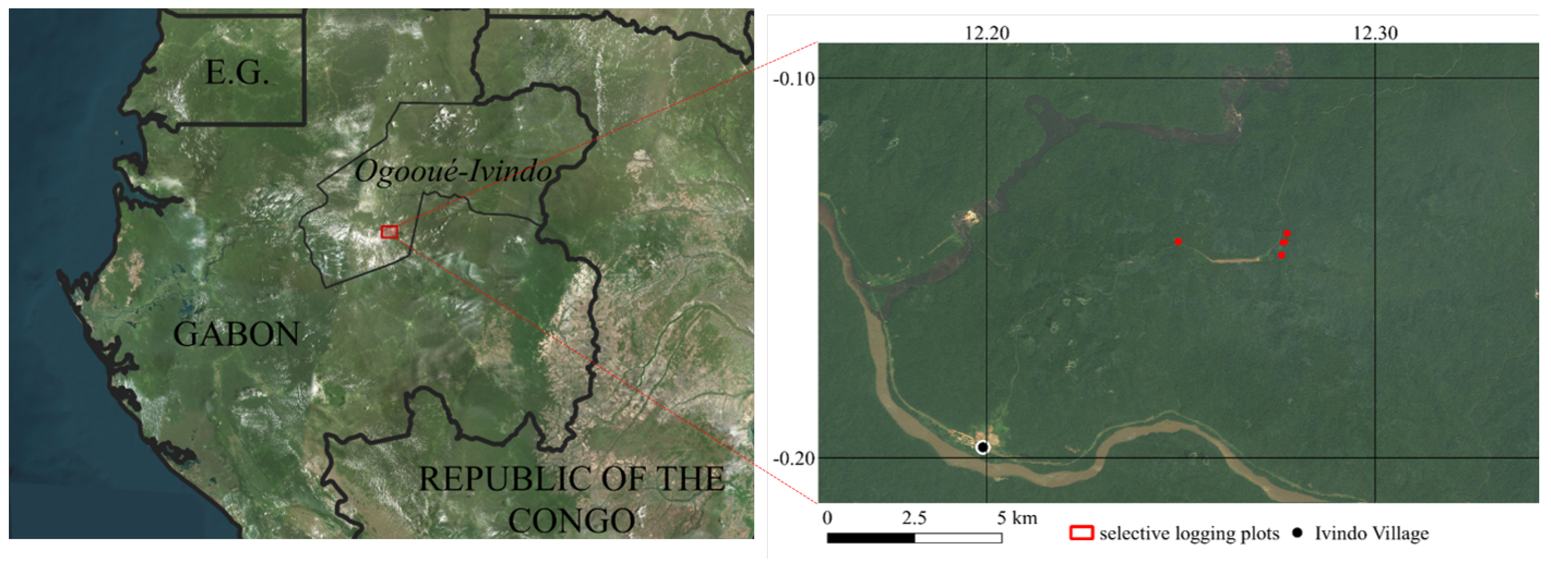
The study site is located around a disused airstrip (0.148°S, 12.264°E) close to the confluence of the Ivindo and Ogooué rivers in the Ogooué-Ivindo department of Gabon (
Figure 1). The nearest settlement, Ivindo village, is also an operational base for logging company Rougier Gabon which holds concessions to extract timber from the surrounding forest, the primary species of commercial value being Okoumé (
Aucoumea klaineana). The logging concession is certified by the Forest Stewardship Council (FSC-C144419).
Mature forest is the dominant landcover in the region, the only exceptions being rivers and some small areas cleared for habitation, agriculture, transport and logging activities. The forest has a stem density in the range of 200 to 300 ha
, and the tallest trees generally reach heights of 40 to 50 m. Regionally, the forest has a high biomass density and relatively low stem turnover (e.g., compared to many Amazonian areas) with annual mortality of trees >10 cm diameter estimated to be about 1% [
33].
Central Gabon is one of the cloudiest regions in the world [
34], and its climate is characterised by a long dry season June–August, during which precipitation is below 1 mm/day, but extensive low cloud cover suppresses temperatures and maintains high humidity [
35]. A second dry season occurs December–February. According to TRMM monthly precipitation estimates [
36], annual precipitation at the study site is less than 2000 mm per year, and has been declining in recent years towards 1500 mm per year or less—a trend also confirmed by nearby ground data [
37].
2.2. TanDEM-X Acquisitions
The TDX mission consists of twin X-band SAR satellites that orbit in close proximity to each other (<1 km, quantified to the nearest mm) following a helix trajectory [
24]. For each bistatic data acquisition by TDX, one satellite (the primary) acts as a transmitter-receiver while the other (the secondary) receives the signal only. The result is therefore a pair of images, representing the signals received by the two satellites. For this study, eight such pairs of images were obtained from the German Aerospace Center (DLR) in coregistered single look slant range complex (CoSSC) format. The CoSSC products were captured using stripmap mode, used horizontal polarisation both in transmission and reception (HH), and had an azimuth resolution of approximately 3 m [
38]. The range resolution, meanwhile, varies according to the bandwidth of the transmitted signal: those acquisitions for which a bandwidth of 150 MHz was possible have a slant range resolution of 1.3 m, while other acquisitions were limited to 100 MHz and have a slant range resolution of 1.9 m [
38].
Table 1 shows the dates, pass directions and bandwidths of the eight CoSSC products in chronological order, indicating also the dates of selective logging in our field plots. The effective perpendicular baseline between the satellites and the corresponding height of ambiguity (HoA; the vertical displacement equivalent to a 2
shift in interferometric phase) are also shown [
18].
For each pass direction, there are two acquisitions before logging and two acquisitions after logging. It should be noted that the descending images were all limited to 100 MHz bandwidth, meaning they have a slightly lower range resolution than the ascending images.
In general, if the HoA is less than or equal to the height of a tree, the interferometric phase contributions from the top and bottom of the tree would differ by over 2
[
26]. As the tree height in the study area rarely exceeded 50 m (our data showed the top canopy height to be less than 50 m for 98% of forested area), and all acquisitions have a HoA greater than this, it is unlikely that such ambiguities will affect our results. We note, however, that HoA magnitudes are smaller and thus ambiguities more likely in the pre-logging acquisitions than the post logging acquisitions, and in the descending passes than the ascending passes.
2.3. Field Data
Forest inventories in four 1 ha plots were conducted in August 2019 and February 2020, to estimate biomass change from controlled selective logging in January 2020. To improve the accuracy of our biomass change estimates, TLS was used to create structural models of all logged trees (prior to felling). Unoccupied aerial vehicle (UAV) laser scanning (LiDAR) data were also obtained immediately before the logging began, and then again one year later, following the removal of logs from the inventory plots and additional logging in the surrounding area. This allowed the creation of eleven control plots of 1 ha each, in which the UAV data showed no significant changes in Top Canopy Height.
2.3.1. Forest Inventories
Four permanent plots were established such that they were easily accessible by UAV from the disused airstrip and contained commercially viable trees. Each plot was rectangular with one side orientated within 10° of North, and an area within 10% of 1 ha. The locations of the plot corners were measured by the integrated GNSS receiver of a Riegl VZ-400 terrestrial laser scanner.
For the pre-logging census, conducted in August 2019, every living tree stem with diameter at breast height (DBH) greater than 10 cm was tagged and given rough coordinates (≈
m) relative to the southwest corner of the plot. At a height of 1.3 m along the stem from the ground a tape measure was used to determine DBH according to the RAINFOR field protocol [
39]. Tree species were determined by local botanists, from which wood density was estimated using a global database [
40]. In addition, each stem was inspected for structural damage, and categorised according to the approximate reduction in wood volume compared to an undamaged stem of the same size (0, 10, 25, 50 or 75%). It was noted if stems were leaning, fallen or showing obvious signs of disease or parasitic damage.
In collaboration with Rougier Gabon, trees were selected for logging such that the plots would span a range of AGB change values, while also providing useful timber. The logging took place between the 24 and 28 January 2020, under special permission from Gabon’s Ministry for the Protection of the Environment and Natural Resources, Forests and the Seas, removing 18 trees in total. The selected trees were felled in the direction which would cause the least damage to other trees, according to standard low-impact logging practice (the concession is certified by the Forest Stewardship Council, license FSC-C144419).
A second census was carried out at the beginning of February 2020, in which all remaining tagged trees were remeasured and reassessed for damage. At this stage, the logs remained in the plots, meaning that later damage is very likely to have occurred upon the extraction of the logs. However, the timing is appropriate for this study as it matches the acquisition of post-logging TDX images.
Wood density for each tree was estimated at the species level from a global database [
41] where possible. Genus averages and local averages were used for trees where an exact species match in the database could not be found. An allometric equation based on destructive harvests across the tropics [
42] was used to convert DBH (
D) and wood density (
) values to AGB according to an environmental stress factor (
E) that averaged −0.096 across the plots. The form of the equation is as follows:
The AGB was adjusted to account for structural damage where this was recorded in the census, and fallen stems were assigned an AGB of zero. The application of this allometry constitutes the main source of error in field based estimates of AGB, as tree-level values have a relative error of around 50% [
42]. Furthermore, it has been found that large trees (DBH > 70 cm) are poorly characterised by this allometry [
43], in part due to the lack of destructive harvest data from large trees, and also due to the large variation in AGB of such trees [
44,
45]. This could have had a strong effect on our biomass change estimates, as only 2–7 trees were removed from each plot, and these had a median DBH of over 100 cm. To avoid this, we used TLS to estimate the AGB of these trees with higher accuracy and less bias [
46].
2.3.2. Terrestrial Laser Scanning
TLS surveys of all four selective logging plots were conducted in August 2019 using a Riegl VZ-400 scanner. For each plot, two scans were obtained at every point on a square 10 m grid aligned with the plot edges—one with the scanner orientated vertically and another with the scanner tilted horizontally to allow for complete (and oversampled) coverage of the hemisphere above each scan location. Highly reflective targets were used for approximate coregistration of the point clouds from successive scan positions, which was fine tuned using a plane-fitting algorithm implemented in Riegl’s RiSCAN PRO software. The TLS acquisition followed the protocol of [
47].
The point clouds of the logged trees were extracted from the coregistered data using an open-source software package called treeseg [
48]. These were then used to create quantitative structural models (QSMs) according to the methods detailed in [
49,
50]. From the QSMs, the AGB of each tree was estimated by multiplying the model volume by wood density. The relative error in TLS derived AGB compared to destructive harvest values can be as low as 3% [
46], although older studies obtained 28% [
43], 23% [
51], and 16% [
50]. From this evidence, even in a worst case scenario TLS provides a considerable accuracy improvement compared to DBH-based allometry. Our final estimate of absolute AGB loss for each plot was given by the sum of the TLS-derived AGB of the logged trees plus the net change in AGB of the other trees as measured in the field survey.
2.3.3. UAV Control Plots
A canopy height change map covering 328 ha of forest around the selective logging plots was derived from UAV LiDAR data collected in January 2020 and January 2021. A RIEGL miniVUX-1DL discrete-return lidar was mounted to a DELAIR DT26X fixed-wing UAV, which was flown at a height of about 140 m above the ground and at an average speed of 17 m/s. A GNSS base station was used for post-processing kinematic (PPK) corrections to the flight paths, which, in combination with ground control points, resulted in point clouds with a geometric accuracy of 1.8 cm. The average point density was 240 pts·m
[
52].
Canopy height maps (CHMs) were derived at a pixel scale of 25 cm by taking the difference between the lowest and highest returns (after noise filtering) in each cell. The difference between the CHMs in 2020 and 2021 was taken to produce a
CHM raster, and resampled to 2 m pixels. In 1 ha regions where fewer than 2% of
CHM pixels were less than −5 m, we randomly selected eleven control plots, as shown in
Figure 2. The control plots are all square and orientated parallel to north. One control plot is situated on bare ground, while the rest are all in forested areas.
2.4. Topography of Field Site
The region covered by TDX acquisitions has elevation varying from about 300 to 700 m, while the area covered by UAV data ranges from 400 to 550 m. These values are according to 1 arc-second SRTM data, which was also used to analyse slope steepness. As shown in
Figure 3, a significant proportion of the area covered by the TDX acquisitions has slope >10°, and the distribution of slopes in the region covered by UAV lidar is representative of this wider region.
The selective logging plots include a reasonable proportion of slopes between 5 and 10°, but are generally flatter than the surrounding topography (
Figure 3). The control plots, meanwhile, contain steeper slopes typical of the region but no completely flat areas. This allowed us to build an empirical model relating TDX
to
AGB in flatter regions (where logging is more likely to occur anyway), while evaluating its stability in steeper regions using the control plots.
2.5. InSAR Data Processing
The Sentinels Application Platform (SNAP) software was used in conjunction with custom Python scripts to process the CoSSC images. All Python scripts written in conjunction with this paper can be accessed on Github at
https://github.com/harrycrstrs/tandex, accessed on 3 November 2021. The first step was to generate interferograms by multiplying the complex pixel values of the primary image by the corresponding conjugate values in the secondary image. This product has an argument equal to the phase difference between the images (the interferometric phase), which—ignoring decorrelation—is a function of the range difference from the target to the two satellites.
Two components of the interferometric phase were estimated and subtracted from the interferograms. The first of these was the theoretical phase that would be obtained from a featureless surface at zero elevation, known as the ‘flat earth’ phase. Secondly, the additional phase due to surface elevation was estimated using the 1 arc-second SRTM DEM [
30]. By subtracting the SRTM phase, we obtained a residual component representing only the difference between SRTM and TDX
. This was beneficial because it reduced the range of phase values to less than
, as SRTM and TDX
should not differ by more than the HoA [
28]. As a result, the process of unwrapping to solve for absolute phase was considerably simplified. In summary, we calculated the phase difference between complex signals
and
and then subtracted the flat earth phase
and topographic phase
as follows:
Noise is present in
over vegetated areas due to volume decorrelation [
53], making it necessary to perform a multilooking step. In this study, we investigated the effect of multilooking on TDX sensitivity to forest disturbance by processing each interferogram with different numbers of looks, achieved by fixing the number of range looks between 3 and 32 and requiring an approximately square pixel in ground coordinates. This corresponded to pixel spacings ranging from 5.3 m (6.0 m ) to 53.4 m (66.5 m) for the ascending (descending) passes. We will refer to results by the number of range looks
as this was the fixed quantity in our processing chain.
Goldstein Phase Filtering [
54] was applied to further reduce phase noise without reducing resolution. The adaptive filter exponent, which controls the strength of the filtering [
55], was set to 0.2 (from a range of 0 to 1). This was kept low because we expected our interferograms to contain high phase gradients—for example around canopy gaps—which may have been smoothed over by strong filtering.
A basic unwrapping algorithm was then applied, under the assumption that no two ‘true’ phase values differed by more than
. This consisted of applying a constant offset
according to Equation (
3), where
i and
j refer to range and slant coordinates.
The optimal value for was estimated by numerically minimising the number of adjacent pixels that differed by more than five radians. This value is equivalent to a height difference of 43 m for the TDX acquisition with the smallest HoA, meaning anything beyond this could reasonably be assumed to be unphysical, considering the UAV data showed trees higher than this to be uncommon.
At this stage, most images contained a systematic phase component dependant on range and azimuth coordinates. This ‘ramp’ is likely due to small errors in orbit information [
26], but can be corrected using standard methods. A random sample of 10,000 points was taken from each image and fitted by least squares to a plane. The plane was then subtracted from the unwrapped phases to give deramped phases according to the Equation (
4), where
,
and
are the parameters of the plane.
The unwrapped, deramped phase values were converted to
by dividing them by the interferometric wavenumber
k. This was calculated on a pixel-by-pixel basis from slant range
and incidence angle
, according to Equation (
5), where
is the effective perpendicular baseline [
56].
Finally, the SNAP tool for range-doppler terrain correction was applied using the SRTM 1 arc-second DEM, thus transforming the images into geographic coordinates.
2.6. Multilooking
A quantitative analysis in [
26] shows that TDX
is typically located within 1 m of the mean height of the X-band radar scattering profile. In the case of a tropical forest, we can relate this to the spatial distribution and sizes of leaves and branches—the higher these scattering surfaces are, the higher
will be. Under the assumption of stable topography, we can therefore relate changes in successive measurements
to changes in vegetation structure. Specifically, we hypothesised that plots with the highest intensity logging and greatest losses of AGB would show the largest reductions in
.
However, changes at the pixel level will occur for a number of reasons, including variations in sensor geometry and movement of scatterers in the canopy. For this reason, it seems desirable to use a large number of multilooks in order to average out these variations. Previous studies examined phase changes at a scale of 50 m [
26,
27]. On the other hand, it is important to recognise that variations in
are related to the vertical structure of tropical forest, rather than being simply ‘noise’, meaning that spatial averaging risks the loss of useful information [
57]. The X-band signal is able to penetrate through small gaps, resulting in a few-look
distribution that correlates strongly with forest height [
28]. Our first analysis, therefore, was to compare relationships between
and
AGB from selective logging at different levels of multilooking, to determine the optimal level for quantification of biomass change. It should be noted here that by multilooking, we specifically refer to spatial averaging of the complex radar signal, as opposed to spatial averaging of
, which was performed in all cases.
We estimated
changes in the logged plots according to Equation (
6), where
and
indicate the mean of pre- and post-logging images, respectively. The sum was taken over all pixels intersecting with a 10 m buffer around the plots, to allow for the fact that some logged trees fell outside of the plot boundaries.
To ensure spatial averaging was performed over the same area at each level of multilooking, all images were resampled using the nearest neighbour method to the coordinates of the first 3 × 3 look ascending image. Although each layer contained an arbitrary constant, no calibration was required because our analysis was concerned only with the spatial variation in . Instead, the resulting constant term in was approximated by assuming the average change over the image was zero. For this part of the analysis, all acquisitions from both pass directions were used.
2.7. Combining Pass Directions
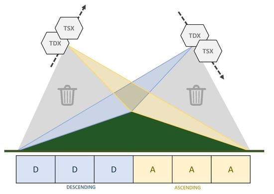
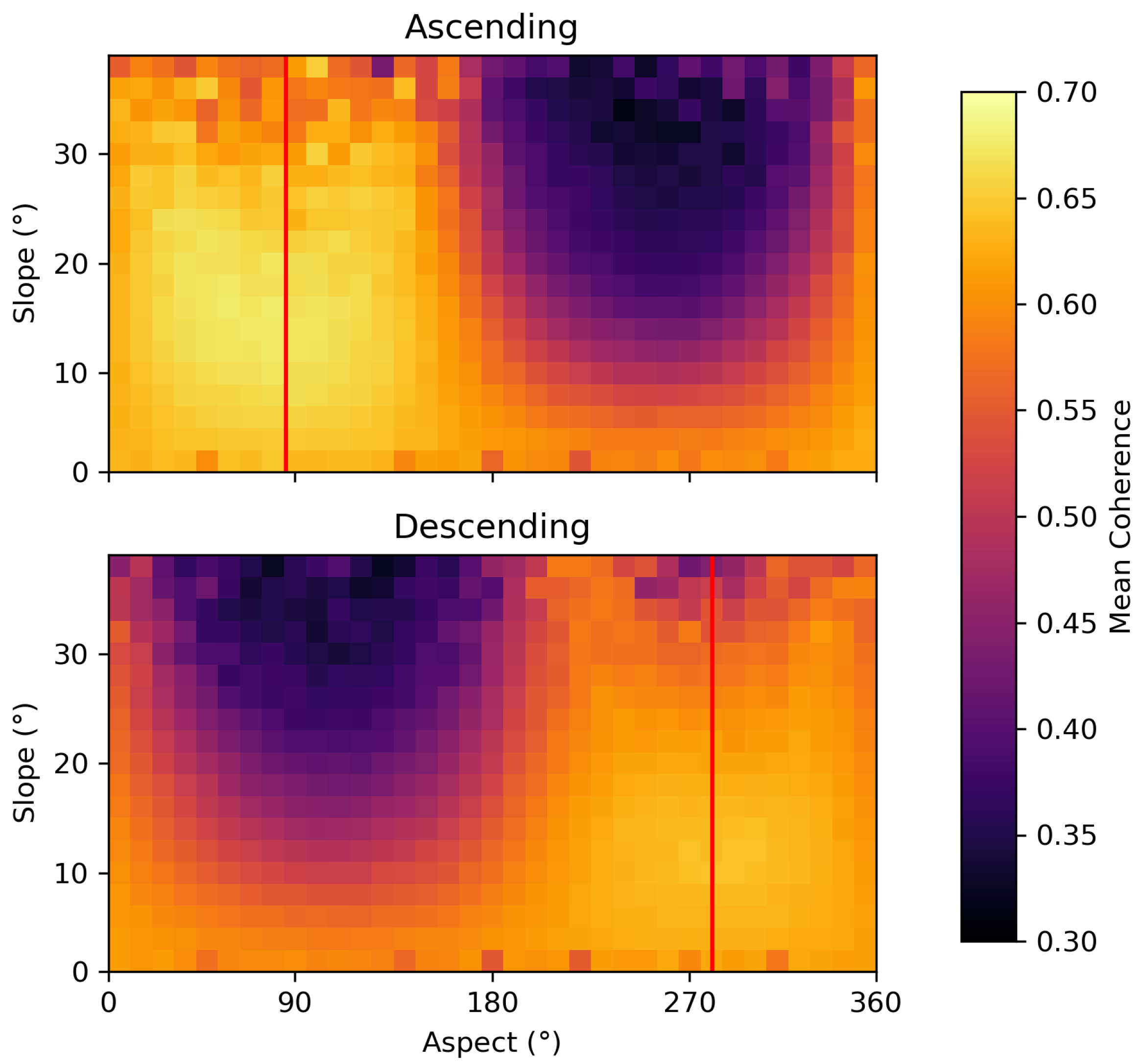
In hilly terrain, it is inevitable that some slopes will face towards the SAR sensor, resulting in small local incidence angles
. This degrades the range resolution on the ground and leads to poor coherence [
58,
59,
60], as reflections from across such slopes are compressed in the slant range direction, as illustrated in
Figure 4a,b.
In contrast, slopes facing away from the SAR sensor with large values of
lead to smaller areas of ground and less vegetation in each range bin, as shown in
Figure 4c,d. Small values of
can be suppressed by fusing data from multiple pass directions: a technique previously shown to improve DEM creation and water body detection using TDX data [
61]. To quantify this, we consider how
relates to viewing geometry and topography. Specifically, it may be expressed in terms of terrain slope from horizontal
S, slope aspect from north
a, sensor azimuth angle from north
z and radar incidence angle to the vertical
.
An illustration of
for fixed
S is shown in
Figure 5a. By the nature of a sun-synchronous orbit (such as the one used by TDX) the azimuth angles for ascending (
) and descending (
) passes are fixed for a given scene. Slope aspect, on the other hand, may be anything between 0 and 360. Therefore, for a given
S, we can write the lower bound of
for each pass.
If we allow the possibility of flexibly choosing either pass for a given slope and aspect, then the minimum value of
can be increased if the ascending and descending curves cross, that is, if there is a value of
a which satisfies:
This equation has a solution when the following condition is met:
In other words, selecting from multiple pass directions mitigates small
for slopes greater than a critical angle, equal to half the difference between the ascending and descending nominal incidence angles. Below this threshold, one pass always has higher
than the other. Intuitively, the magnitude by which
is enhanced will be greatest when
= 180°, that is, when the cosine terms in Equation (
7) for the two passes are perfectly out of phase. In this situation, slopes that face towards the sensor during one pass face away from it during the opposite pass. As sun-synchronous orbits are nearly polar, the reality is not too far away from this ideal condition—for our TDX scenes
. While Equation (
9) has no analytical solution, a numerical result is shown in
Figure 5b, confirming that
enhancement is strongest for the steepest slopes.
To test if pass selection provides more stable results in practice, we estimated degradation across the AOI using four different methods. The first two methods used one acquisition of each pass direction from before and after the selective logging event. For the
naive averaging method, the change in
for each pixel was calculated using data from both pass directions according to:
where the sum is over ascending and descending passes. In contrast, the
pass selection method used the estimated projected local incidence angle (based on SRTM data)
and median coherence values for each pass
to determine which pass direction to use for each pixel, according to the algorithm shown in Equation (
12).
The coherence was used for flatter areas as topographic features <30 m in size may not be well represented in the SRTM data, and because other factors (such as range bandwidth) also have an effect on image quality. Areas that had low coherence in both pass directions ( < 0.4) were masked. In addition, an ascending only estimate was obtained using all four ascending acquisitions, and a descending only estimate was obtained using all four descending acquisitions. For these estimates, pixels for which were masked, and was simply taken as .
For each method, was averaged to a pixel size of 1 ha. Then, a linear model—the parameters of which were determined by comparison to our field data—was used to produce estimates of AGB.
4. Discussion
We found that the selection of the optimal TDX pass direction for each pixel removes the sensitivity of interferometric phase height change () to incidence angle (). In our case, with images spanning about a month, this led to a plausible map of forest degradation over a study area. The measured responded well to the magnitude of change in our field plots, but whether this holds for areas of higher slopes remains currently unvalidated with field data; however, it appears plausible. This suggests that, even in hilly areas, X-band InSAR appears to be a useful method for quantitatively mapping the presence and magnitude of biomass change, provided images are captured from ascending and descending passes. With one pass only, errors on slopes facing the sensor are large, and likely impossible to correct in post-processing.
Unlike the majority of current methods for large-scale degradation mapping, which output binary results [
62], our InSAR approach provides a measure of the magnitude of biomass change (
Figure 7). There is a need for measurements of this kind because countries are required by the Intergovernmental Panel on Climate Change to report the biomass extracted during commercial felling as an immediate carbon emission [
63], regardless of how the timber is subsequently used. A binary indicator of degradation could mask differences in emissions intensity spanning an entire order of magnitude, and such differences are not random: they are driven by the type and intensity of degradation, for example the number of logged trees and reduced impact logging practices. This means that spatial averaging will not be sufficient to estimate carbon losses based on a binary map of degradation. Such maps would therefore force policy makers to assume that regions undergoing the most degradation by area are the most at risk, despite the fact that these regions could be experiencing lower levels of biomass depletion than other regions with localised but more intense degradation. While lidar surveys by UAV or plane can provide more accurate quantitative measures of forest structural change, it is not feasible to make regular surveys spanning the whole of the tropics with these platforms. Spaceborne InSAR, therefore, appears to be a promising approach to fully quantifying carbon emissions from forest degradation.
An additional advantage to our approach is that it can detect changes in humid tropical forests throughout wet and cloudy seasons, during which cloud-free optical imagery is rare. Especially in central Africa and SE Asia, where cloud cover is high all year round, this is vital to producing accurate degradation maps. Relying on optical data could—at best—lead to lag times of a year or more before degradation is detected, and at worst, could result in degradation in cloudy regions being missed entirely.
Our study highlights the uniquely rich data of TDX. It is important, however, to note some limitations of this sensor. The main objective of the TDX mission is to create a worldwide DEM, and as such, its acquisition program is not optimised for tropical forest monitoring. Acquisitions for science applications cannot be requested for particular dates, as they must be taken in the gaps between the systematic DEM acquisitions, meaning that regular repeat times are not guaranteed [
64]. While TDX has already surpassed its design lifetime, it is predicted to continue performing well for several more years [
64], potentially providing more opportunities during the 2020s for experimental acquisitions. A number of new X-band SAR constellations are now being developed commercially (such as Umbra, ICEEYE and Capella Space), but we are not aware of any that will attempt to replicate the bistatic formation of TDX required for coherent interferometry of forests. It may be crucial, then, to make use of this novel imaging mode for scientific purposes while it is available.
4.1. Importance of Multiple Geometries in SAR Acquisition
Our results show that collecting SAR imagery from both ascending and descending passes leads to a transformational improvement in the quality of interferometric data over tropical forests, even in areas of moderate topography. This improvement comes about directly from the multiple viewing geometries (because slopes greater than 10 lead to poor coherence when facing away from the sensor) and is not related to the overall volume of data. If anything, our results suggest that fewer acquisitions with multiple geometries would be far more useful for this application than a dense time series where every image is from the same pass direction.
This finding adds to the list of applications where multiple geometries are known to be beneficial. This includes the use of S-1 SAR shadows to detect patches of tropical deforestation [
20]. Furthermore, Du et al. showed that multiple geometries also leads to improved accuracy in detecting waterbodies with TDX data, as well as creating DEMs in complex terrain, including urban environments [
61]. Multiple passes are also important when using InSAR to precisely track targets in 3D, such as ice flows [
65], artificial reflectors [
66], or geological faults [
67].
Despite this, multiple geometries are not always prioritised by spaceborne SAR acquisition plans. In the case of TDX, a second global DEM is currently being produced, but this relies on a single acquisition for “considerable areas”, meaning that many changes in these regions could be masked by topography [
68]. Furthermore, the S-1 mission only ever collects one pass direction for vast swathes of the Brazilian Amazon and central Africa [
69]. Although bistatic interferometry is not possible with S-1, this still raises the concern that change detection in tropical forests could be adversely affected. To ensure total coverage, future SAR missions should aim to pass over all areas of interest in both directions.
4.2. Importance of Few-Look Interferograms
A strong relationship between TDX and AGB change was obtained by using few-look interferograms. It should be stressed that we still averaged values of to a 1 ha pixel size to generate maps of degradation: our finding is that performing this averaging on the real valued pixels was more effective than averaging the complex valued SAR signal. This suggests that the distribution of single look phases contains valuable information relating to the distribution of scatterers in dense vegetation, and should not be thought of as “noise” to be smoothed out.
The minimum number of looks we tested was , and this gave us the best sensitivity of to AGB. It may be possible to attempt an analysis using even fewer looks or no multilooking at all, but the computational requirements may become disproportionately large. On the other hand, it may be that different levels of multilooking can provide complementary information. Future work could investigate this by using multiple layers to take into account changes across different scales.
Our finding is in agreement with a previous study that used few-look TDX interferograms to estimate forest height [
28]. This was achieved by approximating the ground phase as
, where
was the mean and
the standard deviation of phase values over an area of 1 ha. Our results show that few-look interferograms are useful not just for estimating the ground elevation, but also for detecting structural changes throughout the vegetation profile.
4.3. Evaluation of Predicted Biomass Loss Maps
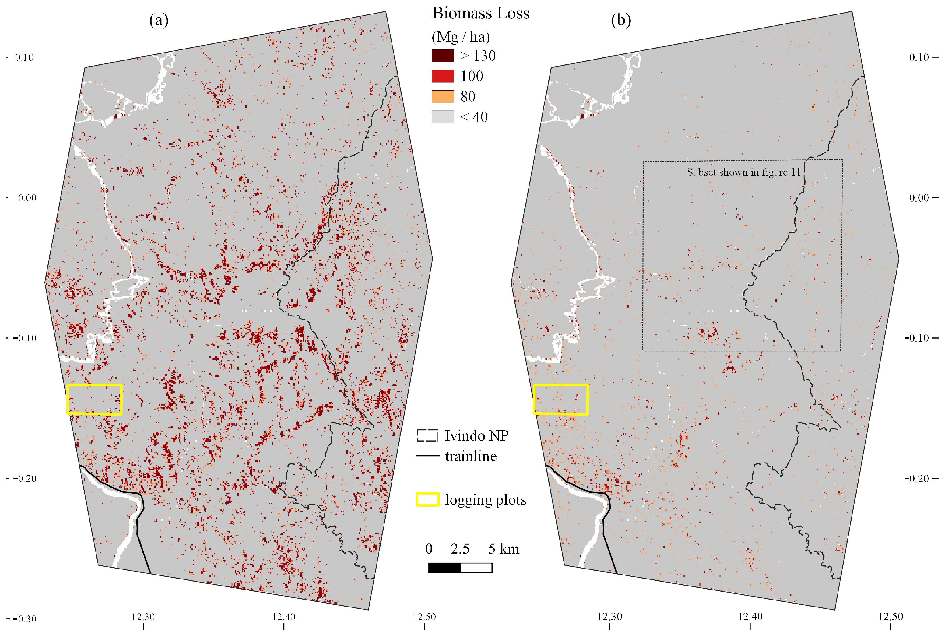
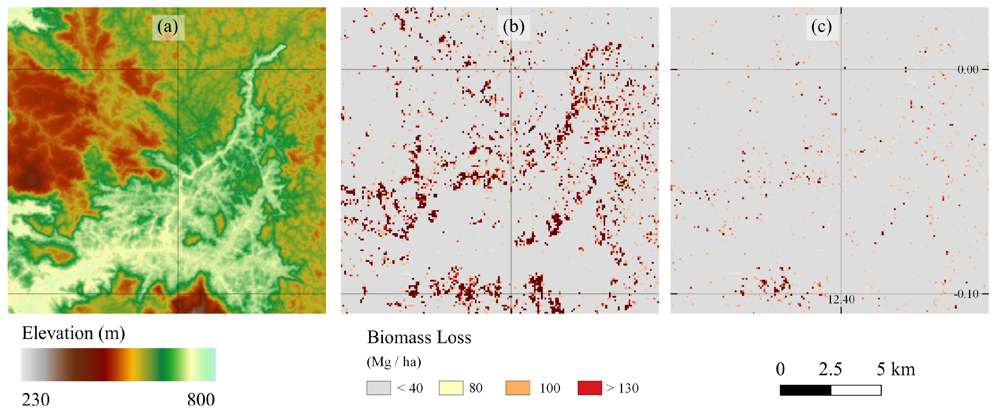
In addition to demonstrating the importance of multiple pass directions and few-look interferograms, we also extrapolated our method to the area of 115,370 ha over which the ascending and descending TDX passes overlapped. A cluster of severe biomass loss is discernible in the predicted map (
Figure 10b) around (12.4, −0.1). We are aware that logging operations were happening outside of the controlled plots at the time of the TDX acquisitions, in a limited geographical area to their north and east. While the cluster of loss may correspond to those logging operations, no data on their precise location has been published yet. Outside of this cluster, the map mostly indicates a random distribution of small disturbances which could realistically occur naturally as larger trees die, as well as a concentration of degradation in close proximity to the section of railway line leading to Ivindo village, where additional human disturbances might be expected due to accessibility.
Some topographic effects do still persist when using the pass selection method, although they are less pronounced than when using the naive method (
Figure 10a). These residual effects are illustrated in
Figure 11, where spatial patterns of biomass loss match regions of steep topography. Additional artifacts are present where changing water levels may have exposed islands in the wide rocky rivers, but it is possible to mitigate these using a forest/non-forest mask.
4.4. Comparison to Other Forest Disturbance Products
Here we make a brief comparison of our results to the RAdar for Detecting Deforestation (RADD) disturbance alerts [
19]. This product maps and estimates the date of disturbances greater than 0.2 ha in size by detecting changes in S-1 backscatter [
19]. Although S-1 has a lower resolution than TDX at around 20 m [
70], it provides the advantage of regular repeat passes (every 12 days over our study area) which allow long time series to be analysed. S-1 data is also publicly available and has global coverage, giving it huge potential for large-scale forest monitoring.
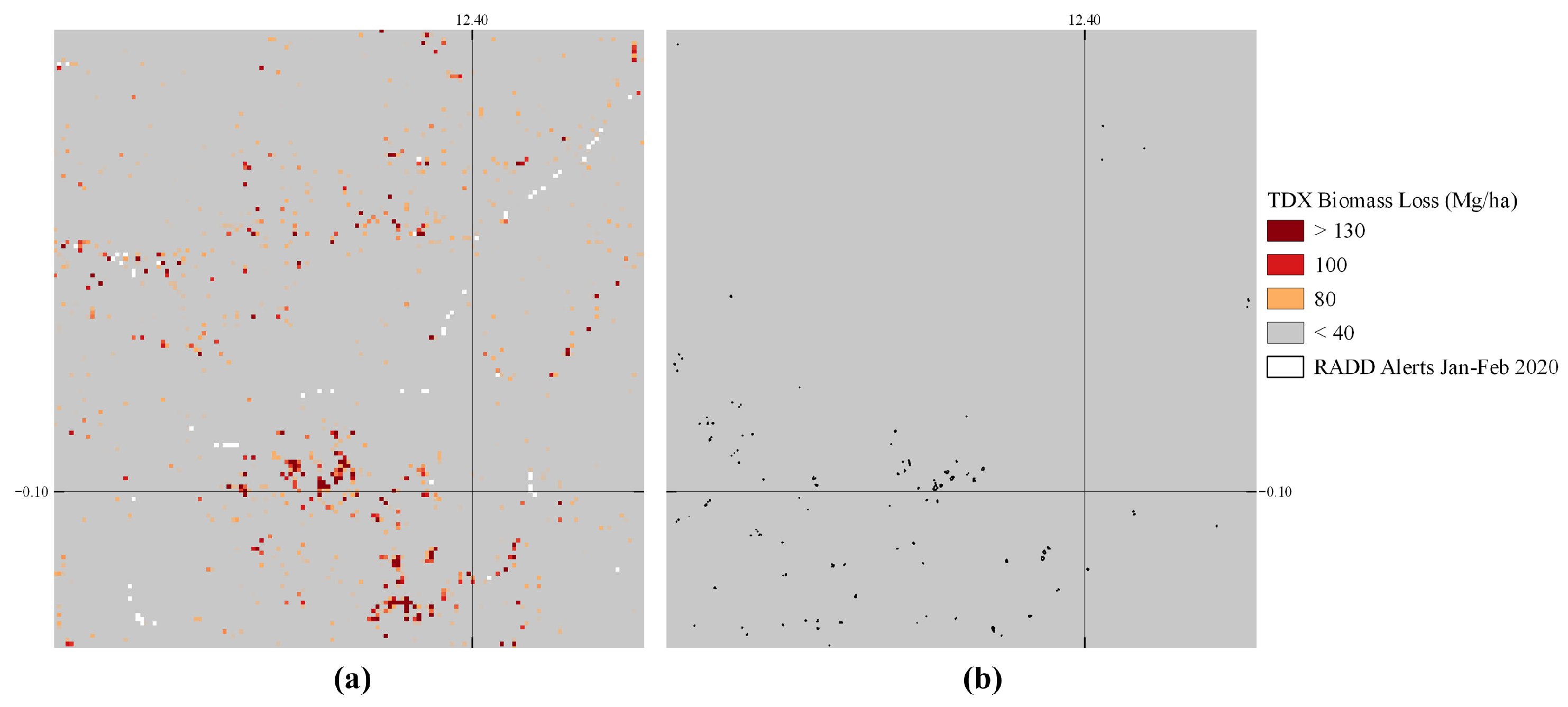
We compared RADD disturbance alerts from January 2020 onwards to our TDX derived estimates of degradation, using
looks and the pass selection method. In the cluster of degradation visible around the centre of our TDX scene which may be associated with logging activity, we found disturbances that were a spatial match across both data sets (see, for example,
Figure 12).
Overall, 11.6% of RADD alerts in the first half of 2020 coincided with areas where TDX
was less than −1.5 m, compared to a baseline of 1.5% across the study area, further suggesting some crossover in the events being detected by the two approaches. We included a time period extending beyond our final TDX acquisition to account for the fact that the statistical method used to generate RADD alerts may lead to late detections [
19]. On the other hand, the remaining 88.4% of TDX degraded area was not captured in the RADD alerts. This is likely to be due in part to the ability of TDX to pick up disturbances smaller than the 0.2 ha minimum mapping unit in the RADD product, which was comparatively insensitive to low level degradation. We found the RADD product was most sensitive to degradation events that caused TDX
to decrease by around 2 m or more, as shown in
Figure 13. Although
exceeded this 2 m threshold for two of our measured plots, the RADD alerts did not detect those events, suggesting that selective logging events of this kind are not spatially continuous enough to present as a disturbance greater than 0.2 ha, despite the fact that more than five large trees were removed from each hectare of forest.
In addition, our biomass loss map is likely to contain commission errors due to phase noise and topographic effects. Unfortunately, quantifying the rate of commission error would only be possible given a high-resolution degradation dataset of known accuracy, which does not yet exist for our study area. We can show, however, that TDX predicts a wider area of forest disturbance than the RADD alerts. This is demonstrated in
Table 4, where for comparison we also include the University of Maryland (UMD) forest loss product [
32] generated using optical data from the Landsat missions.
As expected, the UMD product detects much less disturbance than the radar products, as it is cloud limited and operates at too coarse a pixel size (30 m) to quantify selective logging. Our method using TDX appears to detect much more widespread forest disturbance than the RADD alerts, and this ratio is dependent on the temporal accuracy of the RADD alert dates (which is unknown) and the phase height decrease that is defined in this scenario as a disturbance. This comparison is somewhat limited by the fact that the TDX data use the statistics of a region to estimate a continuous variable (biomass loss), while the UMD and RADD systems work by classifying individual pixels as either disturbed or undisturbed. Nevertheless, it is clear that TDX phase height could have the potential to reveal lower intensities of forest degradation than these products if the false alarm rate is properly quantified.
4.5. Limitations
While our method has been shown to reduce topographic artifacts in TDX
, it is yet to be shown whether it provides accurate estimates of
AGB in areas where degradation and steep slopes coincide. The local angle of incidence should affect the penetration of X-band radar into canopy gaps, with steeper
leading to deeper penetration [
28]. It would therefore be expected that the relationship between
and
AGB is in turn parameterised by
. For this to be tested, temporally matching ground change data over steep slopes and satellite data would be required. Although our UAV lidar coverage includes steep terrain, no TDX acquisitions from the time of the second field campaign (January 2021) were available for comparison.
A further limitation of our AGB estimates is that they are restricted to a small range of values (losses between 40 and 130 Mg·ha). This is again due to the nature of our field data, which consisted of plots which lost up to 130 Mg of AGB. To obtain accurate estimates of landscape scale biomass change, an important step will be to include reference measurements spanning the full range from deforestation to forest regrowth. Furthermore, a larger number of ground based measurements are required to improve the statistical significance of the relationship we found. To do so, follow-up studies at this site should utilise the multi-temporal UAV lidar as a stepping stone between field measurements and satellite imagery.
In order for our method to be applicable in other regions, two other points must be considered. Firstly, in our plots, small numbers of large, merchantable trees were felled, which reflects one type of degradation seen in tropical forests, but does not match the structural changes typical of, for example, understorey clearing, fire, fuel-wood harvesting or road construction. As these changes remove different components of the forest at different heights, they will be likely to have a different effect on TDX
. Therefore, to develop a general degradation model, reference measurements should include alternative forms of degradation. Secondly, we have not considered in this study the importance of initial forest height and structure. Modelling suggests the magnitude of
AGB for a given
is heavily dependent on forest height [
28]. Studies across different tropical forest types will therefore be necessary to develop a generalisable model of
AGB, and methods of estimating forest height from satellite products, such as using GEDI-TDX fusion [
71], will also need to be refined.
5. Conclusions
TDX is a remote sensing variable capable of measuring the relative magnitude of selective logging events in a dense tropical forest. We found a linear relationship (r > 0.99) between and biomass change in four plots where AGB varied from −28 Mg·ha to −131 Mg·ha. The variation in amongst eleven control plots suggested that the minimum detectable change was approximately −40 Mg·ha.
Fewer looks of the radar signal (before calculating ) leads to the best sensitivity to forest degradation. We found the strongest relationship between and AGB was obtained for the smallest number of looks that was tested (). In this case, we found a sensitivity of 2.3 cm decrease per Mg of AGB lost, which was greater than for any larger number of looks. The standard deviation of amongst the control plots was 66 cm, which was more stable than for any larger number of looks.
If only a single-pass direction is available, steep terrain leads to large magnitude artifacts due to decorrelation on the slopes facing towards the SAR sensor. Neither ascending only or descending only passes showed more stability over our control plots than any method using both passes, even when the total number of images used was fixed. This can be attributed to a rapid loss of coherence with slope steepness for aspects differing from the azimuth angle by more than 90.
Where multiple pass directions are available, they can be most effectively utilised through a pixel-by-pixel pass selection algorithm. The issue of decorrelation on sensor-facing slopes can be mitigated because these regions will face away from the sensor when it is passing in the opposite direction. We designed an algorithm that chose to estimate either from ascending or descending acquisitions, based on estimated projected local incidence angle and coherence. Our pass selection algorithm performed significantly better than a simple averaging of pass directions, producing a map of degradation that was less biased by topography, more stable at the pixel level, and more plausible considering our knowledge of the study area. The accuracy of our predicted map of AGB could not be quantified due to a lack of suitable validation data, either ground or remote sensing based, but we compared it to the S-1 based RADD forest disturbance alerts and found that it suggested a higher level of degradation.
Finally, our results demonstrate that few-look TDX interferograms contain valuable information about forest structure, and highlight the vital importance of multiple SAR viewing geometries for InSAR mapping of degradation across the hilly regions of the world’s tropical forests.


 ,
, 


