Measurement of Aspect Angle of Field-Aligned Plasma Irregularities in Mid-Latitude E Region Using VHF Atmospheric Radar Imaging and Interferometry Techniques

Abstract

Multireceiver and multifrequency radar imaging were carried out with the 46.5 MHz MU radar in Japan (34.85°N and 136.10°E) to examine the aspect sensitivity of field-aligned plasma irregularities (FAIs) in the mid-latitude ionosphere E region. A radar beam was directed to geographic north and at 51° zenith angle, which was normal to the geomagnetic field line around 100 km height. Nineteen receivers and five carrier frequencies were used for radar imaging to retrieve the power distribution in the radar volume, and then the aspect angle along the geomagnetic field line was calculated according to the angular power distribution. Retrieval algorithms such as Fourier, Capon, and norm-constrained Capon (NC-Capon) were employed, in which the NC-Capon was applied to FAIs for the first time and found to be more suitable for the present study. The aspect angles estimated by the NC-Capon ranged between 0.1° and 0.4° mostly, and averaged around 0.2°, which were the same order to the previous measurements with radar interferometry (RI), made for equatorial electrojet irregularities and the lower mid-latitude sporadic E region. For comparison, RI-estimated aspect angles were also investigated and found to be close to that of NC-Capon, but distributed over a wider extent of angles.

1. Introduction

Aspect sensitivity of refractive irregularities in the atmosphere describes a dependence of radar echo intensity on angular direction. In horizontally structured atmosphere, the radar echoes are usually strongest near the zenith and drop off with off-zenith angle, which is evident in observations throughout the low and middle atmosphere with the radar at MF, HF, and VHF bands. For the field-aligned plasma irregularities (FAIs) in the ionosphere, however, the radar echoes are strongest at the beam direction normal to the geomagnetic field line, and decay very quickly with off-perpendicular angle along the geomagnetic field line. Aspect angle is a measurement of aspect sensitivity, which can be defined by the half width of half power, or the standard deviation of Gaussian fitting in the angular power distribution; the former is about $\sqrt{ln4}$ (≒1177) times the latter if the angular power distribution is characterized by a Gaussian function. The order of aspect angle in the lower atmosphere is within several degrees [1,2]. By contrast, it can be as small as several times 0.1° or less in FAI echoes, depending on latitude and height [3,4,5,6]. It has been addressed in [3,4,5,6] that the FAIs’ aspect angle in the direction of geomagnetic field line relates partly with the values of electron-neutral collision frequency (ν_e), electron gyrofrequency (Ω_e), ion-neutral collision frequency (ν_i), ion gyrofrequency (Ω_i), the ratio ν_e/Ω_e, among others, and moreover, is also subjected to nonlinear coupling process of unstable waves in the plasma irregularities.

Because of highly localized FAI echoes in the radar volume, and much, much smaller aspect angle in the ionosphere than in the lower atmosphere, many of the approaches/techniques proposed for measurement of aspect angle in the lower and middle atmosphere, such as those used in [1,2,7,8,9,10,11,12,13] (i.e., beam swing, spaced antenna, spectral width, etc.), are difficult to apply to FAIs. A proper approach to measurement of FAIs’ aspect angle is the radar interferometry (RI) technique that was first applied to equatorial ionosphere by Kudeki and Farley [3] and observed the aspect angles of electrojet irregularities ranging between 0.1° and 0.4° generally. A later study for equatorial spread F irregularities found an even smaller value of aspect angle, i.e., a few times 0.01° [4]. Additionally, RI was applied to the lower mid-latitude sporadic E region (~25.6°N and ~120.8°E geography; ~16.33°N and ~167.34°W in geomagnetic coordinate) but with a different process and definition [14], in which the aspect angles of layer-type and clump-type plasma irregularities were estimated, and were found to be the same order of magnitude as that of equatorial electrojet irregularities.

In this study, we attempted to apply the approach of coherent radar imaging (CRI) to estimate the aspect angle of mid-latitude E region FAIs. CRI has been employed for study of aspect sensitivity in the lower and middle atmosphere [2,15,16]. The technical requirement of CRI is the use of separate antennas as independent receiving channels to collect the radar echoes. The multiple-channel echoes received can be employed to retrieve the in-beam angular power distribution through a beamforming process. The algorithm of beamforming can be linear-based, e.g., the Fourier method, or adaptive, such as the Capon [15] and norm-constrained Capon methods [17,18,19,20], and others. CRI can be regarded as an advanced version of RI.

To meet the requirement of CRI, the Middle and Upper (MU) Atmosphere radar, a pulsed radar operated at 46.5 MHz and maintained by Kyoto University, Japan, was employed in this study. The MU radar is located at 34.85°N and 136.10°E in geographic coordinates, and 26.36°N and 153.78°W in geomagnetic coordinates. A total of 25 receiving channels can be assigned, and moreover, frequency hopping of five carrier frequencies between radar pulses is available. Such flexible capabilities of operation allow radar image processing not only in 1D range imaging and 2D angular imaging, but also 3D spatial imaging. To this end, the retrieval methods used consistently, such as the Fourier, Capon, and norm-constrained Capon methods, were examined to find their suitability for the present study. As far as we know, the norm-constrained Capon method has not yet been applied to full 3D radar imaging. In addition to radar imaging, several sets of subarrays aligned approximately with the direction of the geomagnetic field line are also available to test the RI technique in measurement of aspect angle. Therefore, comparison of measurements is possible to validate the usability of radar imaging and RI, or evaluate which kind of method is more suitable for estimating the aspect angle of FAIs with the MU radar configuration. To complete the study, the effect of signal-to-noise ratio (SNR) on the estimate of aspect angle was also examined.

The rest of this paper is organized as follows. In Section 2, measurement techniques are described, including experimental setup and data processing of radar imaging and RI. Section 3 provides the results and discussion, and Section 4 states the conclusions.

2. Measurement Techniques

Radar experimental setup, radar imaging, and radar interferometry are described in Section 2.1, Section 2.2 and Section 2.3, respectively.

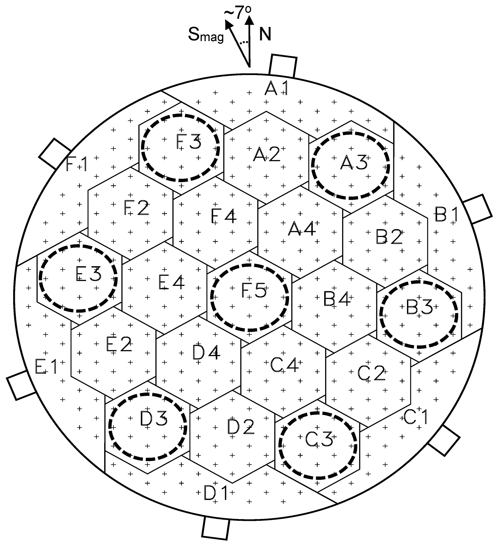
2.1. Radar Experimental Setup

Figure 1 shows the antenna array configuration of the MU radar, in which each plus symbol denotes a single antenna with an independent transceiver. The diameter of the array is about 103 m and the array can be partitioned into 25 subarrays, as denoted by the letters from A1 to F5. The separation of adjacent subarrays is 19.55 m, and central carrier frequency is 46.5 MHz. A detailed description of the radar characteristics can be found through the website http://www.rish.kyoto-u.ac.jp/English/MU/index.html (accessed on 25 December 2021). Some operational parameters related to the present study are described below and listed in

Table 1. Radar parameters.

Parameters	Values
Beam direction	Geographic north, 51° zenith
Interpulse period (IPP)	0.0015 s
Pulse length	4 μs
Sampling time step	4 μs
Number of sampling gates	128
Integration times	1
Pulse codes	no
Carrier frequencies	46.25, 46.375, 46.5, 46.625, and 46.75 MHz
Receiver channels	Full array and 19 subarrays A2–F5, exclusive of A1, B1, C1, D1, E1, F1
Sampling range (height)	120.0–196.8 km (~75.518–123.850 km)

.

Full array was used for transmission of radio waves, and the radar beam was steered to geographic north and at the zenith angle of 51°. As a result, the radar beam bearing was perpendicular to the geomagnetic field line around the height of 100 km. Moreover, five carrier frequencies were employed in sequential radar pulses that were operated repeatedly. In reception, the whole array and the 19 subarrays in the interior of the array were assigned to 20 receiving channels to collect the radar echoes from five different carrier frequencies. This multireceiver and multifrequency operation allows us to execute 1D range imaging, 2D angular imaging, and 3D spatial imaging. The imaging here means the retrieval of power distribution within the radar volume.

The sampling range interval was between 120.0 and 196.8 km. The corresponding sampling height interval was between about 75.518 and 123.850 km, which was estimated by projecting the sampling range at vertical direction and ignoring the curvature of the Earth surface. Sampling time was 0.0075 s for each carrier frequency returns (=5 × IPP = 5 × 0.0015 s). In calculation of covariance function for radar imaging, 256 raw data points were taken for ensemble average, resulting in an estimate of 1.92 s (=256 × sampling time = 256 × 0.0075 s).

2.2. Radar Imaging

The retrieval methods used for radar imaging in this study were Fourier, Capon, and norm-constrained Capon. We compared their effectiveness for deriving aspect angle in the 2D and 3D imaging processes. For 2D angular imaging, only multireceiver data are needed. For 3D spatial imaging, both multireceiver and multifrequency data are required. These methods of radar imaging were examined and employed in several studies in the research field of atmosphere [15,16,17,18,19,20,21,22,23,24,25]. A brief mathematical description of the radar imaging employed in this study is provided in Appendix A.

Two-dimensional angular imaging yields the power density (termed brightness distribution hereafter) as a function of angle for each sampling gate, and there could be more than one local maximum in the brightness distribution. Nevertheless, only the one with the maximum brightness level was used in the study. That is, the mean location of the brightness center encircled by the highest contour level was determined first, and then Gaussian-function fitting was applied to the brightness values around the estimated mean location of the brightness center to obtain a brightness width, i.e., the Gaussian-fitted standard deviation. The fitting was executed only in the direction along the geomagnetic field line, the aspect angle of which we surveyed. It was estimated that the geomagnetic south pole was about 7° west of geographic north in the field of view of the MU radar in the observation. Therefore, it was expected that the brightness distribution of FAI echoes is field-aligned and usually has a slant of about 7° in the 2D imaging surface viewed from the radar beam direction [25]. Notice that the imaging surface is the transverse plane of the radar beam, and the origin is at the radar beam bearing. Abscissa and ordinate of the imaging surface are zonal and elevation directions relative to the radar beam bearing, respectively (Figure 2b,c; explained later).

Since the aspect angle of FAIs could be as small as only 0.1~0.5°, the imaging was processed with an angular step of 0.05° in both zonal and elevation directions. To confirm the Gaussian-fitting result, we also used the peak-find process built in the computing software (i.e., MATLAB) to obtain the half-power peak width. The half-power peak width or the Gaussian-fitted standard deviation is an indication of the aspect angle of the FAIs, in which the former is about $\sqrt{ln4}$ (≒1177) times the latter if the angular brightness distribution around the mean location of the brightness center, in the geomagnetic field-aligned direction, is characterized by a Gaussian function.

It should be noticed that the aspect angle estimated from 2D angular imaging is a mean value within the range interval of the sampling gate. If one expects to observe the spatial structure and estimate the aspect angles at different ranges in the radar volume, 3D spatial imaging is one of the solutions. In the 3D radar imaging executed in this study, the range step of imaging was 37.5 m, giving 17 range locations in the sampling gate of 600 m length, i.e., at the range locations of −300, −262.5, −225, …, 300 m relative to the range center of the sampling gate. A smaller range step is certainly available, but it consumes more computation time and may not be helpful for improving the range resolution due to the finite number of carrier frequencies used in observation. For each range location, the Gaussian fitting and peak-find process can be performed for the 2D-angular brightness distribution to obtain two brightness widths in the geomagnetic field-aligned direction, which denote two possible values of aspect angles at that range location. The results from 19 subarrays and 7 subarrays (indicated by the dashed circles in Figure 1) are compared and shown later.

2.3. Radar Interferometry

Radar interferometry (RI) has been widely used in atmospheric studies such as mean angle of arrival of radar echoes [26], lightning detection [27], meteor radar wind [28], among others. Use of RI in measurement of the aspect angle of FAIs was first reported by Kudeki and Farley in 1989 [3] for the equatorial electrojet region. In their approach, normalized cross spectra were calculated for all receiver pairs and then a suitable fitting of a parabola to the absolute values (termed coherence) of the cross spectra was made to retrieve aspect angles at various spectral lines (i.e., Doppler shifts). Lu et al. [6] extended the study of [3] and provided the following normalized cross spectrum:

$$S_{mn}\left(k{D}_{mn},w\right)=e^{jk{D}_{mn}⟨\theta {⟩}_w}\exp \left[-\frac{1}{2}{k}^2{D}_{mn}^2{\theta }_{rms}^2\left(w\right)\right],$$

(1)

where k is wave number, w is Doppler shift, D_mn is the length of the baseline between receiver antennas m and n, ⟨θ⟩_w is the mean angular location of the irregularity pattern at the Doppler shift w, and θ_rms(w) denotes the angular spread value relative to ⟨θ⟩_w, which can be regarded as the aspect angle at w. Gaussian function is then employed to fit the coherence of the cross spectra to derive the parameter θ_rms.

In this study, we did not examine the aspect angle at different Doppler shifts. Therefore, the cross-correlation function S_mn(kD_mn) was estimated in time domain. Unfortunately, there was no set of subarrays with the baseline parallel to the direction of the geomagnetic field line exactly. As shown in Figure 1, the three subarrays (A2, F5, D2) and the two sets of five subarrays (A2, F4, F5, D4, D2; A2, A4, F5, C4, D2) had the alignments of about 7.60° east of geographic north, and thus had about 14.85° difference from the geomagnetic southern pole. Another set of subarrays, F3, F4, F5, C4, and C3, was aligned in the direction of about 28.07° west of geographic north, and thus had a difference of about 20.82° from the geomagnetic south pole. These sets of subarrays were used for RI in this study.

3. Results

The aspect angles retrieved from radar imaging and RI are shown and discussed in this section. Moreover, the effect of SNR on the estimate of aspect angle is also examined.

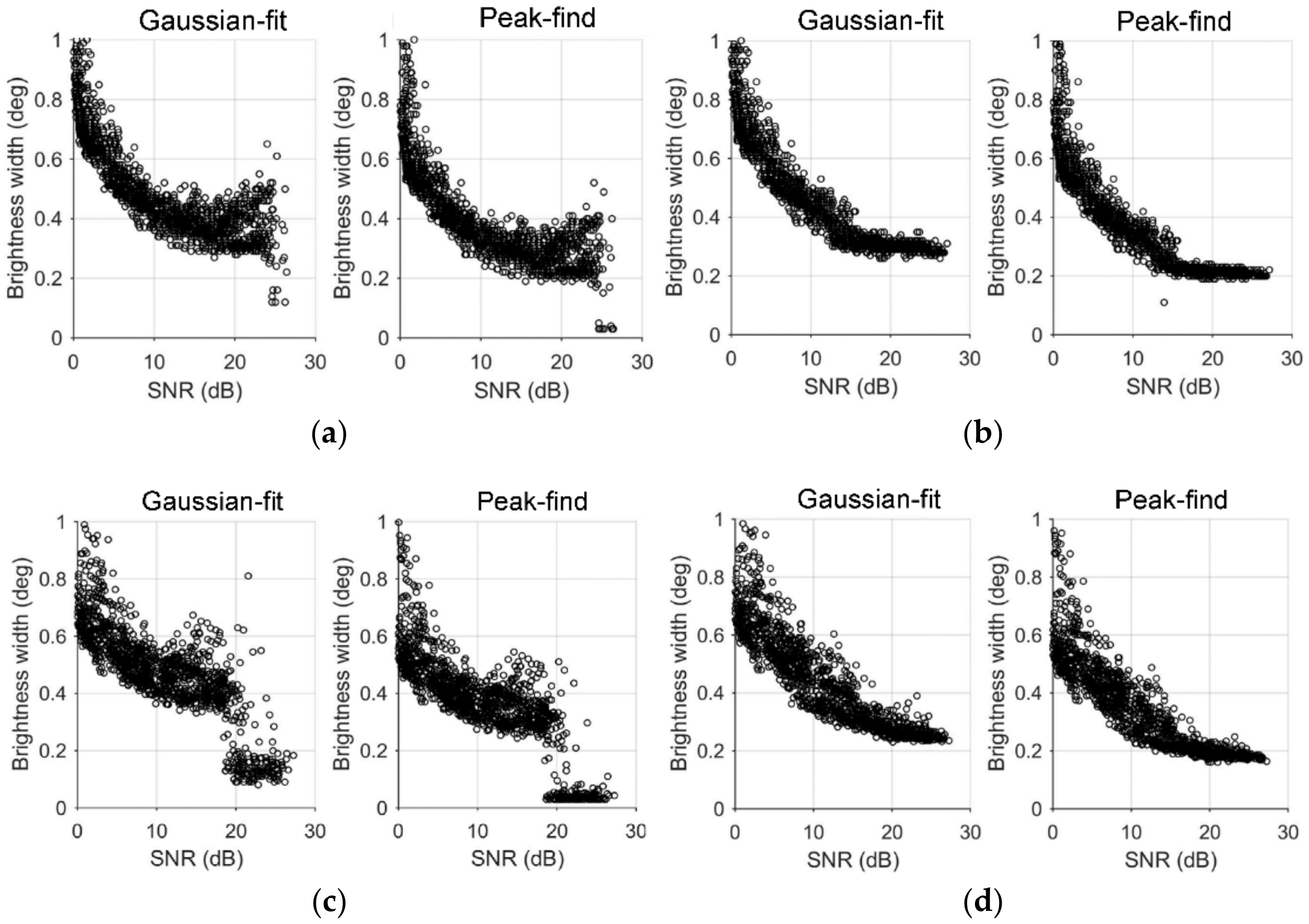
3.1. Radar Imaging in 1D, 2D, and 3D

First, the benefits and shortages of the Fourier, Capon, and NC-Capon methods in 2D and 3D radar imaging were investigated, as shown in Figure 2. Figure 2a shows the radar echoes collected by the full array of the radar, where the original range-time intensity of FAIs is present in the left panel and 1D range-imaging result is displayed in the middle panel. In the range imaging, the radar echoes collected from the full array and five carrier frequencies were processed with the standard Capon method, and the range step was 5 m. It is clearly seen in the range-imaged brightness distribution that these FAI echoes were positive range rate, indicating a northern component of motion. This direction of motion can be revealed from the typical range–Doppler spectrum of the echoes provided in the right panel of Figure 2a. As shown, the Doppler velocities spread out over a wide range, but were negative mostly and centered on −100 m/s, indicating a motion of away from the radar site according to our definition of Doppler velocity direction in calculation. Since the tilted radar beam was directed to geographic north, apparently a northern component of motion existed in the FAIs structure. Certainly, the zonal motion might also contribute a part to the Doppler spectrum, but could not be as large as 100 m/s because the radar beam was directed to geographic north and had a very narrow beamwidth (~3.6°). Notice that some visible spectral power at the Doppler velocities of around 200 m/s and in the range interval between 164 and 166 km were aliases of some negative Doppler velocities that were smaller than the negative Nyquist velocity (about −215 m/s).

Figure 2b shows 2D angular brightness distributions of two examples retrieved from different methods. The value given in the title of the Fourier panel is SNR in linear scale, and following the SNR value is the data time on 26 July 2019 (hh:mm:ss LT). Obviously, the first example shows that the Fourier and Capon methods were not good for retrieving the brightness distribution (present in dB scale). The Fourier result had a coarser angular resolution and suffered from serious contamination of sidelobes arising from the weighting vector used in retrieval (refer to the Appendix A). The Capon result, on the other hand, provided an unreliable distribution, which is known to be related to the sensitivity of the method to small errors in the received signals. Nevertheless, the Capon method is still workable for many of the echoes, as shown in the example displayed in the second row of Figure 2b. By contrast, the NC-Capon method exported more stable and reliable outcomes, and moreover, a larger δ value yielded a higher angular resolution. A comparison of the results from different δ values is given later. Readers can also find the meaning of the δ value in Appendix A.

Figure 2c shows two examples of the angular brightness distributions in 3D imaging retrieved from different methods. The upper two rows provide two slices of brightness distribution at the range position of 150 m and 0 m in the sampling gate, and the bottom row presents the brightness distribution at the central position (0 m) of the sampling gate in another example. In general, the features resulting from different methods were similar to that in 2D imaging.

Figure 3 shows the scatter plots of brightness width (degree) vs. SNR (dB). The outcomes of Gaussian fitting and peak-find methods, 2D and 3D imaging, and Capon and NC-Capon methods are present, where the δ value in the NC-Capon method was 60. In this study, we define the half width of half power as representative of aspect angle, and therefore the brightness width obtained from Gaussian fitting was multiplied by $\sqrt{ln4}$. This correction was also made for the results of the RI technique shown later. The brightness centers with angular locations within 2° of the radar beam direction were adopted, and moreover, the scatter plots of 3D imaging included only the brightness widths from the slices of angular distributions at the range positions of −75, −37.5, 0, 37.5, and 75 m in the sampling gate. The reason for this selection of outcomes is shown later in Figure 4. Several findings from Figure 3 are listed below:

• Brightness width was SNR-dependent; generally, a larger SNR produced a smaller brightness width.
• The brightness widths retrieved from the Capon method (Figure 3a,c) were more divergent at higher SNR as compared with the result of NC-Capon (Figure 3b,d), regardless of 2D or 3D imaging, and in Gaussian fitting or peak-find processes. Moreover, a sudden drop of brightness width at large SNR can be seen in the Capon result. This drop, together with divergence of brightness widths at larger SNR, implied a failure in using the Capon method for these cases.
• As revealed from the outcomes at higher SNR, Figure 3b,d shows that Gaussian-fitted brightness widths were about 0.1° larger than those of the peak-find method.

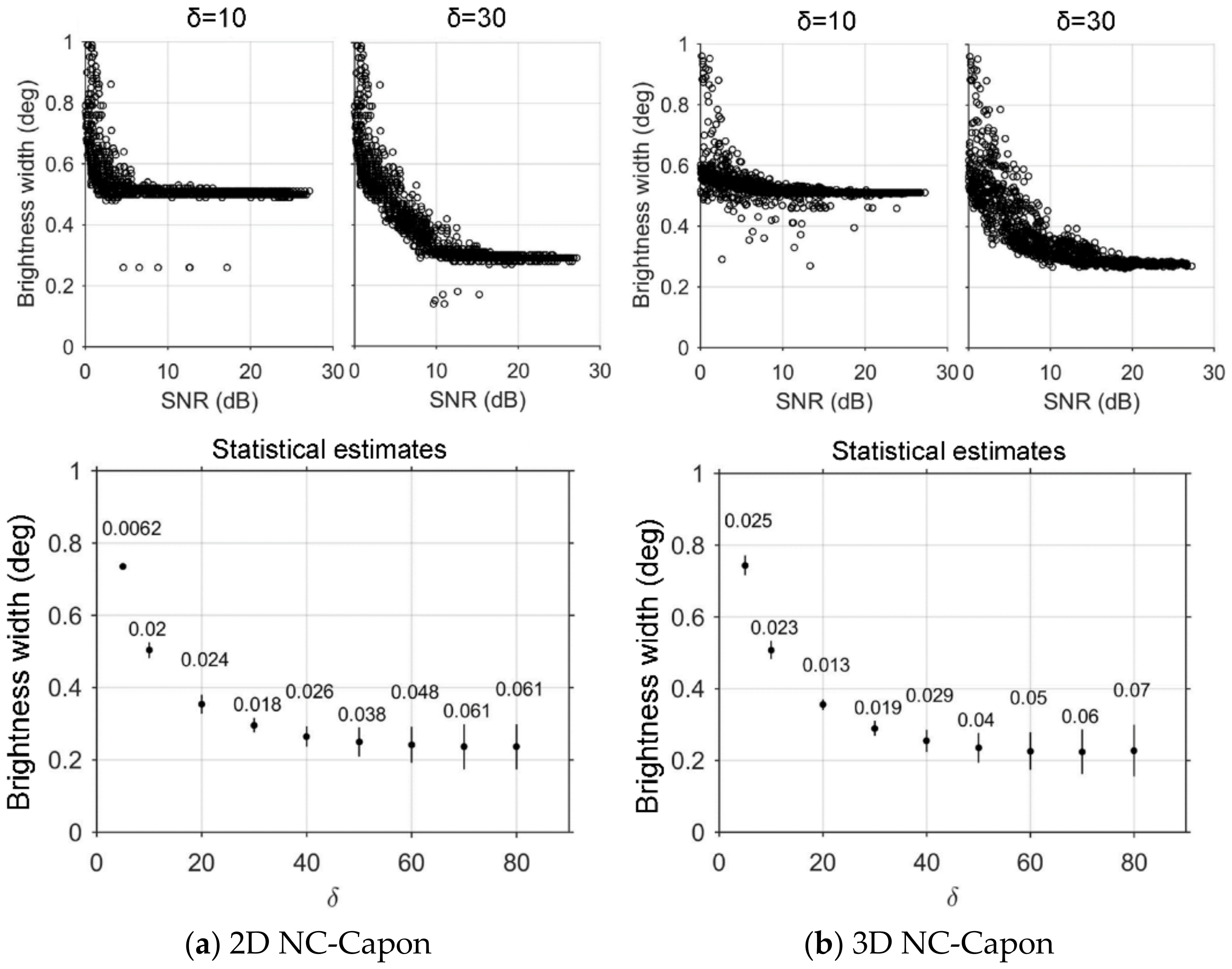
Figure 3. Scatter plots of brightness width (aspect angle) vs. SNR, retrieved from Capon and NC-Capon methods: (a,b) show 2D radar imaging results obtained from Capon and NC-Capon methods, respectively. The parameter of δ is 60 in NC-Capon method. (c,d) are similar to (a,b) but show 3D radar imaging results. Both outcomes of Gaussian-fit and peak-find methods are present.

Figure 3. Scatter plots of brightness width (aspect angle) vs. SNR, retrieved from Capon and NC-Capon methods: (a,b) show 2D radar imaging results obtained from Capon and NC-Capon methods, respectively. The parameter of δ is 60 in NC-Capon method. (c,d) are similar to (a,b) but show 3D radar imaging results. Both outcomes of Gaussian-fit and peak-find methods are present.

Figure 4. Profiles of brightness widths obtained from the NC-Capon method with three different δ values (20, 40, and 60). The brightness widths for statistical estimates are collected with the threshold of (a) SNR > 1 and (b) SNR > 20; g₁ to g₅ indicate the range center locations of five sampling gates.

Figure 4. Profiles of brightness widths obtained from the NC-Capon method with three different δ values (20, 40, and 60). The brightness widths for statistical estimates are collected with the threshold of (a) SNR > 1 and (b) SNR > 20; g₁ to g₅ indicate the range center locations of five sampling gates.

Based on the consequences of what is shown in Figure 2 and Figure 3, the NC-Capon method is definitely more suitable than the standard Capon method for retrieval of brightness width and thereby aspect angle. In the rest of this paper, therefore, only the results of the NC-Capon and peak-find methods are present. Readers can find additional maps of brightness distribution via the web link provided in [29].

As mentioned, in the scatter plot of 3D imaging, only the outcomes from the five slices of angular distributions at the range positions of −75, −37.5, 0, 37.5, and 75 m in the sampling gate were included. This was based on the features shown in Figure 4, where the profiles of mean brightness widths within five sampling gates are shown for three δ values: 20, 40, and 60. The left and right panels demonstrate the results from the outcomes with SNR > 1 and >20, respectively. The horizontal bar denotes the width of two times the standard deviation of brightness width. It can be seen clearly in the left panel that in each sampling gate, the mean value of brightness width varied with the range and had a smaller value around the central range of the sampling gate (indicated by g₁ to g₅). If a higher threshold of SNR was used, i.e., SNR > 20 as given in the right panel, the dependence of brightness width on the range in the sampling gate existed still although the dependence was mitigated significantly. One cause of this characteristic could be the volume weighting effect. In this study, range-weighting and beam-weighting effects were not corrected in either 2D or 3D imaging. This is under the consideration that the echoes of the FAIs are highly localized, and therefore correction of the weighting effect could produce overcorrected brightness values around the edge of the radar volume. To avoid the influence of the weighting effect on estimate of brightness width, we used the outcomes with the brightness centers located around the center of the sampling gate, that is, the range interval within −75 and 75 m, and the angular interval between −2° and 2°.

Figure 4 shows that mean brightness width varied with the δ value used in the NC-Capon method. In view of this, a dependence of the outcome on δ value should be examined further to find a suitable value of δ for the following data analysis. Figure 5a shows the results from the 2D NC-Capon method, where the upper two panels are the scatter plots of brightness width vs. SNR resulting from the δ values of 10 and 30. Obviously, the brightness width at larger SNR decreased with increased δ value. To reduce the influence of SNR, therefore, the outcomes with SNR > 10 were used to estimate mean brightness width, and the results are shown in the lower panel of Figure 5a. As seen, the change of mean brightness width was tiny when the δ value was larger than 40, although the standard deviation of brightness widths increased slightly with δ value. Similar behavior can also be found in the 3D NC-Capon results, as shown in Figure 5b.

More issues of the NC-Capon method that deserve inspection are computation time and brightness value at different δ values. Figure 6 provides an example of 3D NC-Capon showing the variations of brightness sum and computation time with δ value, where the values on ordinate are self-normalized. Note that the brightness sum in panel (a) was the summation of brightness values in the radar volume just from a single estimate; the other estimates had similar scenarios (not shown). On the other hand, the computation time shown in panel (b) was recorded from fifty estimates. As seen, the self-normalized brightness sum decreased with increased δ value, and had tiny changes at the δ values larger than ~40. Meanwhile, the computation time also decreased quickly with increased δ value.

Based on the investigation results shown in Figure 5 and Figure 6, we can use the value larger than 40 for δ to save much computation time, but should not be too large to avoid magnifying the divergence of brightness widths. In view of this, the consequences of δ = 60 are presented in the remaining discussion of the 2D and 3D NC-Capon methods.

3.2. SNR Effect

As seen in the scatter plots of brightness width vs. SNR shown in Figure 5, a lower SNR led to a larger brightness width. In many previous studies, finite correction of SNR effect for the coherence of the covariance function had been suggested to improve the consequences. Usually, this can be made through multiplying the coherence by (1 + 1/SNR₁)^1/2(1 + 1/SNR₂)^1/2, in which SNR₁ and SNR₂ are the respective SNRs of the two data sets used in the analysis. Such a correction will increase the coherence. However, a smaller SNR magnifies the coherence greatly, and could lead to a coherence larger than 1 sometimes, which is irrational and may cause the coherence matrix to be more singular, or lead to improper Gaussian fitting in the RI approach. In view of this, only the coherence with SNR > 1 was corrected, and moreover, the corrected coherence was assumed to be 0.99 when it was larger than 1.

Figure 7a,b provides the comparisons of original and SNR-corrected results of 2D and 3D imaging, respectively. The original scatter plots of 2D and 3D imaging show a significant decrease of brightness width with SNR for the echoes of SNR < ~15 dB. After SNR-correction, the dependence of brightness width on SNR was mitigated appreciably in the 2D imaging result, as shown in Figure 7a. By contrast, SNR-corrected coherence yielded less alleviation of SNR-dependent features in the 3D imaging result, as shown in Figure 7b.

Based on the consequences shown in Figure 7, it is suggested that the outcomes with SNR > 10 dB or even >15 dB can be adopted to calculate the brightness width of the echoes. On the condition of SNR > 10 dB, most of the aspect angles, represented by brightness widths, spread from ~0.15° to ~0.4°. This order of magnitude is consistent with the RI measurements of aspect angles at the equator [3,6] and lower mid-latitude E region [5,14].

3.3. Radar Interferometry

As mentioned in Section 2, four sets of subarrays in the MU radar array, of which baselines are aligned approximately with the direction of the geomagnetic field line, are available for radar interferometry (RI). To compare with the results of radar imaging, however, expression (1) without the factor of Doppler shift was employed. Figure 8 exhibits the results, where the scatter plots of brightness width vs. SNR are shown. Several features can be found in Figure 8:

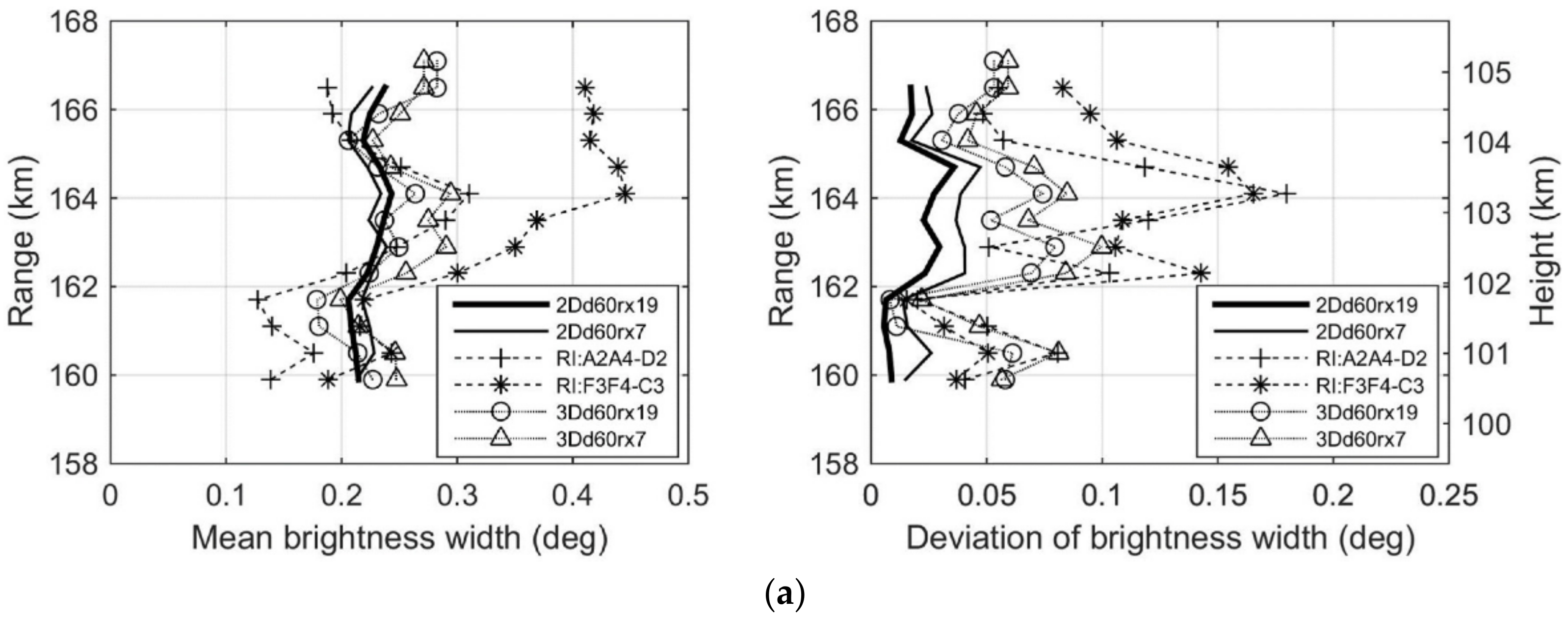
• The scatter plots from the original coherence values show that brightness widths were SNR dependent, as seen in the left subpanels of panels (a)–(d). The scenario was similar to that of 2D and 3D imaging shown in Figure 7. Nevertheless, there were more outliers than in 2D and 3D imaging, i.e., more divergent in the distribution.
• Correction of the SNR effect indeed reduced the brightness width significantly, as shown in the right subpanels of panels (a)–(d). Many brightness widths at lower SNR were now closer to the events at higher SNRs. However, brightness widths still spread over a wider interval of angle than in 2D and 3D imaging.
• The outcomes of the two sets of subarrays shown in (b) and (c) were more concentrated than in (a) and (d), although the baselines of the subarrays of (b) and (c) were not exactly linear.

Figure 8. Scatter plots of brightness width vs. SNR resulting from the radar-interferometry approach proposed by [3]. Four sets of receiving subarrays are used, as indicated in the panels (a–d). Left and right subpanels of each panel show the outcomes from the original and SNR-corrected coherence functions, respectively.

Figure 8. Scatter plots of brightness width vs. SNR resulting from the radar-interferometry approach proposed by [3]. Four sets of receiving subarrays are used, as indicated in the panels (a–d). Left and right subpanels of each panel show the outcomes from the original and SNR-corrected coherence functions, respectively.

For feature (3), it can be understood that (b) and (c) have more subarrays than (a), and the baselines of (b) and (c) are parallel to the direction of the geomagnetic field line more than that of (d). Accordingly, the subarrays in (b) and (c) are more suitable for retrieval of aspect angle of FAIs. As for the features (1) and (2), the aspect angles have more outliers and spread in a broader interval of angle as compared with 2D and 3D imaging results; one of the causes could be the certainty that the baselines of subarrays did not align with the geomagnetic field lines exactly, and another cause was the smaller length of baselines between subarrays. The maximum length of baseline was about 70 m in the subarrays used in Figure 8a–c, and about 80 m in Figure 8d, which were much smaller than that used in [3] and [6] (~310 m).

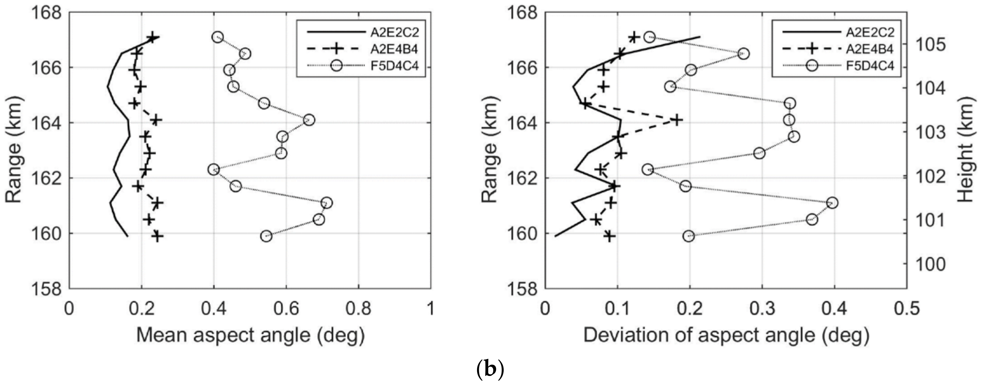
3.4. Statistical Comparison of Aspect Angles

Since different methods may result in different brightness widths (i.e., aspect angles), we compared their brightness widths, as shown in Figure 9. In panel (a), the results from 2D and 3D imaging with 19 subarrays and 7 subarrays (legend “…rx19” and “…rx7”, respectively), and RI (legend “RI:…”) are shown. The 7 subarrays used here are indicated by the dashed circles in Figure 1. The two sets of subarrays for RI are those used in Figure 8c,d. Correction of the SNR effect has been made for coherence and the threshold of 10 dB was given for SNR to select the outcomes for statistical calculation. The δ value was 60 in the NC-Capon method. As a result, the profile of mean brightness width denoted by RI:A2A4-D2 in panel (a) had smaller values than the others below the range of 162 km, while that denoted by RI:F3F4-C3 had the largest values above the range of 162 km. In addition, both mean profiles of RI were more range-variant than other profiles. On the other hand, the standard deviations of RI aspect angles were mostly larger than the others above 162 km, as observed in the right panel of Figure 9a. In the study, we also checked the RI results from the set of subarrays E3, E4, F5, B4, and B3, of which baseline alignment turns aside from the direction of the geomagnetic field line more than that of the subarrays present here, and found that the resultant aspect angles spread over a much broader interval of angle (not shown). It is thus demonstrated that the aspect angles resulting from RI are highly dependent on the baseline alignment of the subarrays. In contrast to the RI results, the mean profiles of 2D imaging, denoted by “2Dd60rx19” and “2Dd60rx7”, had the smallest variation through the range, and moreover, the standard deviations of brightness widths of 2D imaging were generally the smallest among the results. There was not much difference between the mean profiles of “2Dd60rx19” and “2Dd60rx7”, but the standard deviation marked by “2Dd60rx7” had values slightly larger than that of “2Dd60rx19”, suggesting that a smaller number of subarrays may deteriorate the outcomes of 2D imaging. On the other hand, 3D imaging provided consequences approximately between 2D imaging and RI results. In general, the outcomes of 3D imaging resulting from 19 subarrays were closer to that of 2D imaging.

Another outcome of aspect angle estimated from the definition of Wang et al. [14] is provided in Figure 9b. The method of [14] was also based on RI but three non-coplanar receiving antennas/subarrays were used to derive a mean echo center in the radar volume. These locations of echo centers obtained were generally geomagnetic field-aligned. The aspect angle was then defined to be half the angle subtended by the field-aligned length of echo center locations. There are many associations of three receiving subarrays available in the MU radar array. Among them, the results from the three sets of subarrays—A2E2C2, A2E4B4, and F5D4C4—are shown, which are typical and represent larger, medium, and smaller triangle configurations of receiving subarrays, respectively. Note that the abscissa scale in panel (b) is twice that in panel (a). Obviously, the estimated aspect angles depend on the baseline length between receiving antennas, in which a larger triangle configuration yielded smaller and more concentrated values of aspect angles (solid curves). The smallest triangle configuration (F5D4C4) provided the largest mean and most divergent outcomes (circles). In quantitative analysis, the mean aspect angles of the medium triangle configuration (A2E4B4) were around 0.2°, which were closer to those of 2D radar imaging. The largest triangle configuration (A2E2C2), however, produced mean aspect angles less than 0.2° and close to 0.1° at some heights; these were the smallest values among all results. Nevertheless, the deviations of aspect angles yielded by the largest and medium triangle configurations mostly ranged between 0.05° and 0.2°, which were comparable to those in panel (a) but still lager than the results of 2D radar imaging (<0.05°).

Based on the comparison made in Figure 9, 2D radar imaging can yield the brightness width/aspect angle of FAIs varying with range more smoothly and converging on smaller interval. It should be known, however, that the outcome from 2D imaging is an average throughout the range of the sampling gate (600 m in the present study); 3D imaging, on the other hand, is likely to be capable of inspecting the variation of aspect angle or irregularity structure within the sampling gate. A problem for 3D imaging is that its computation time is much longer than that of 2D imaging, especially when using the NC-Capon method. A test shows that the computation time of 3D imaging can be about 150 times that of 2D imaging. The iteration number in the computation of the NC-Capon method is unpredictable because it depends on the characteristics of the individual data set. In addition, the more subarrays employed and more slice numbers given in the processing, the more time consumed in computation, although using more subarrays and slice numbers for radar imaging may export a higher resolution of brightness distribution.

4. Conclusions

In this study, radar imaging and radar interferometry (RI) techniques were applied to the measurement of the aspect angle of field-aligned plasma irregularities (FAIs) in the mid-latitude ionospheric E region. This was achieved by means of multireceiver and multifrequency capabilities built in the Middle and Upper (MU) Atmosphere radar (34.85°N and 136.10°E) of Japan. The brightness distribution retrieved from 2D and 3D radar imaging with three retrieval methods, i.e., Fourier, Capon, and norm-constrained Capon, were investigated. It was shown that the norm-constrained Capon method could produce more reliable brightness distribution for most circumstances and thereby yield a more trustworthy value of aspect angle.

By taking the radar data of SNR > 10 dB for 2D and 3D radar imaging, the estimated mean aspect angles ranged from 0.2° to 0.3°, and the standard deviations of aspect angles were less than 0.1° and could be as small as 0.01° at some heights for 2D radar imaging. These values are consistent with those measured in the equatorial electrojet (EEJ) region and in the lower mid-latitude E region with RI technique. With the MU radar, the RI results are also acceptable for certain receiving configurations, but the derived aspect angles spread over an angular range wider than that of radar imaging. This is attributed to a much shorter baseline used for RI in the MU radar array, as compared with the radar used for the EEJ region, and/or different approaches/definitions of aspect angle made for the lower mid-latitude E region.

In conclusion, 2D radar imaging with the norm-constrained Capon method is preferable to other methods, examined in this study, for measurement of aspect angle with the MU radar configuration. Three-dimensional radar imaging is also recommended for further studies of variation in aspect angle and irregularity structure in the radar volume. Nevertheless, 3D radar imaging with the norm-constrained Capon method consumes a much longer time in computation, which is not advantageous to a great amount of data analysis for the ionosphere. In the future, variations of aspect angle with time and altitude can be investigated with 2D radar imaging for the mid-latitude ionosphere. The results can assist in understanding the spatial and temporal characteristics of plasma irregularities in the ionosphere within the radar volume and at the temporal resolution of instrument integration time.

References

1. Hocking, W.K.; Fukao, S.; Tsuda, T.; Yamamoto, M.; Sato, T.; Kato, S. Aspect sensitivity of stratospheric VHF radar wave scatterers, particularly above 15-km altitude. Radio Sci. 1990, 25, 613–627. [Google Scholar] [CrossRef]
2. Chen, J.-S.; Furumoto, J. Measurement of atmospheric aspect sensitivity using coherent radar imaging after mitigation of radar beam weighting effect. J. Atmos. Ocean. Technol. 2013, 30, 245–259. [Google Scholar] [CrossRef]
3. Kudeki, E.; Farley, D. Aspect sensitivity of equatorial electrojet irregularities and theoretical implications. J. Geophys. Res. 1989, 94, 426–434. [Google Scholar] [CrossRef]
4. Farley, D.T.; Hysell, D.L. Radar measurement of very small aspect angles in the equatorial ionosphere. J. Geophys. Res. 1996, 101, 5177–5184. [Google Scholar] [CrossRef]
5. Huang, C.-M.; Kudeki, E.S.; Frank, J.; Liu, C.-H.; Röttger, J. Brightness distribution of mid-latitude E region echoes detected at Chung-LI VHF radar. J. Geophys. Res. 1995, 100, 14703–14715. [Google Scholar] [CrossRef]
6. Lu, F.; Farley, D.T.; Swartz, W.E. Spread in aspect angles of equatorial E region irregularities. J. Geophys. Res. 2008, 113, A11309. [Google Scholar]
7. Briggs, B.H. Radar measurements of aspect sensitivity of atmospheric scatterers using spaced-antenna correlation techniques. J. Atmos. Terr. Phys. 1992, 54, 153–165. [Google Scholar] [CrossRef]
8. Hooper, D.; Thomas, L. Aspect sensitivity of VHF scatterers in the troposphere and stratosphere from comparison of powers in off-vertical beams. J. Atmos. Terr. Phys. 1995, 57, 655–663. [Google Scholar] [CrossRef]
9. Worthington, R.M.; Palmer, R.D.; Fukao, S. Complete maps of the aspect sensitivity of VHF atmospheric radar echoes. Ann. Geophys. 1999, 17, 1116–1119. [Google Scholar] [CrossRef]
10. Palmer, R.D.; Larsen, M.F.; Fukao, S.; Yamamoto, M. On the relationship between aspect sensitivity and spatial interferometric in-beam incident angles. J. Atmos. Sol. Terr. Phys. 1998, 60, 37–48. [Google Scholar] [CrossRef]
11. Tsuda, T.; VanZandt, T.E.; Saito, H. Zenith-angle dependence of VHF specular reflection echoes in the lower atmosphere. J. Atmos. Sol. Terr. Phys. 1997, 59, 761–775. [Google Scholar] [CrossRef]
12. Chu, Y.-H.; Chao, J.-K.; Liu, C.-H.; Röttger, J. Aspect sensitivity at tropospheric heights measured with vertically pointed beam of the Chung-Li VHF radar. Radio Sci. 1990, 25, 539–550. [Google Scholar] [CrossRef]
13. Zecha, M.; Bremer, J.; Latteck, R.; Singer, W.; Hoffmann, P. Properties of midlatitude mesosphere summer echoes after three seasons of VHF radar observations at 54°N. J. Geophys. Res. 2003, 108, 8439. [Google Scholar] [CrossRef]
14. Wang, C.-Y.; Chu, Y.-H.; Su, C.-L.; Kuong, R.-M.; Chen, H.-C.; Yang, K.-F. Statistical investigations of layer-type and clump-type plasma structures of 3-m field-aligned irregularities in nighttime sporadic E region made with Chung-Li VHF radar. J. Geophys. Res. 2011, 116, A12311. [Google Scholar] [CrossRef] [Green Version]
15. Palmer, R.D.; Gopalam, S.; Yu, T.-Y.; Fukao, S. Coherent radar imaging using Capon’s method. Radio Sci. 1998, 33, 1585–1598. [Google Scholar] [CrossRef]
16. Chilson, P.B.; Yu, T.-Y.; Palmer, R.D.; Kirkwood, S. Aspect sensitivity measurements of polar mesosphere summer echoes using coherent radar imaging. Ann. Geophys. 2002, 20, 213–223. [Google Scholar] [CrossRef] [Green Version]
17. Chen, J.-S.; Wang, C.-Y.; Su, C.-L.; Chu, Y.-H. Meteor observations using radar imaging techniques and norm-constrained Capon method. Planet. Space Sci. 2020, 184, 104884. [Google Scholar] [CrossRef]
18. Hashiguchi, H.; Manjo, T.; Yamamoto, M. Development of Middle and Upper atmosphere radar real-time processing system with adaptive clutter rejection. Radio Sci. 2018, 53, 83–92. [Google Scholar] [CrossRef]
19. Nishimura, K.; Nakamura, T.; Sato, T.; Sato, K. Adaptive Beamforming Technique for Accurate Vertical Wind Measurements with Multichannel MST Radar. J. Atmos. Ocean. Technol. 2012, 29, 1769–1775. [Google Scholar] [CrossRef]
20. Kamio, K.; Nishimura, K.; Sato, T. Adaptive sidelobe control for clutter rejection of atmospheric radars. Ann. Geophys. 2004, 22, 4005–4012. [Google Scholar] [CrossRef]
21. Yu, T.-Y.; Palmer, R.D. Atmospheric radar imaging using multiple-receiver and multiple-frequency techniques. Radio Sci. 2001, 36, 1493–1503. [Google Scholar] [CrossRef]
22. Hassenpflug, G.; Yamamoto, M.; Luce, H.; Fukao, S. Description and demonstration of the new Middle and Upper atmosphere radar imaging system: 1-D, 2-D, and 3-D imaging of troposphere and stratosphere. Radio Sci. 2008, 43, RS2013. [Google Scholar] [CrossRef]
23. Yu, T.-Y.; Furumoto, J.; Yamamoto, M. Clutter suppression for high-resolution atmospheric observations using multiple receivers and multiple frequencies. Radio Sci. 2010, 45, 1–15. [Google Scholar] [CrossRef]
24. Chen, J.-S.; Furumoto, J.; Yamamoto, M. Three-dimensional radar imaging of atmospheric layer and turbulence structures using multiple receivers and multiple frequencies. Ann. Geophys. 2014, 32, 899–909. [Google Scholar] [CrossRef] [Green Version]
25. Chen, J.-S.; Wang, C.-Y.; Chu, Y.-H.; Su, C.-L.; Hashiguchi, H. 3-D radar imaging of E-region field-aligned plasma irregularities by using multireceiver and multifrequency techniques. IEEE Trans. Geosci. Remote Sens. 2018, 56, 5591–5599. [Google Scholar] [CrossRef]
26. Lin, F.-F.; Wang, C.-Y.; Su, C.-L.; Shiokawa, K.; Saito, S.; Chu, Y.-H. Coordinated observations of F region 3 m field-aligned plasma irregularities associated with medium-scale traveling ionospheric disturbances. J. Geophys. Res. Space Phys. 2016, 121, 3750–3766. [Google Scholar] [CrossRef]
27. Yin, W.; Jin, W.; Zhou, C.; Liu, Y.; Tang, Q.; Liu, M.; Chen, G.; Zhao, Z. Lightning detection and imaging based on VHF radar interferometry. Remote Sens. 2021, 13, 2065. [Google Scholar] [CrossRef]
28. Su, C.-L.; Chen, H.-C.; Chu, Y.-H.; Chung, M.-Z.; Kuong, R.-M.; Lin, T.-H.; Tzeng, K.-J.; Wang, C.-Y.; Wu, K.-H.; Yang, K.-F. Meteor radar wind over Chung-Li (24.9°N, 121°E), Taiwan, for the period 10–25 November 2012 which includes Leonid meteor shower: Comparison with empirical model and satellite measurements. Radio Sci. 2014, 49, 597–615. [Google Scholar] [CrossRef] [Green Version]
29. Supplementary Brightness Maps of Radar Imaging. Available online: https://drive.google.com/drive/folders/1u-2wSzr5jdeMzXG7F_ZC0I-8SziWtoJC?usp=sharing (accessed on 27 August 2021).
Figure 1. Configuration of MU radar array. Each plus symbol denotes a single antenna with an independent transceiver. The diameter of the array is about 103 m, and the subarrays denoted by the letters from A1 to F5 are individual receiving arrays. The 19 subarrays in the interior and the seven subarrays encircled are employed in radar imaging. The geomagnetic south pole (Smag) is about 7° west of geographic north.
Remotesensing 14 00611 g001
Figure 2. One-, two-, and three-dimensional radar imaging. (a) Left: radar echoes; middle: 1D range imaging; right: one example of range-Doppler spectrum; (b,c) are the brightness distribution obtained from 2D and 3D radar imaging with Fourier, Capon, and norm-constrained Capon methods, respectively. Two examples are shown. Brightness values in (b,c) are self-normalized and displayed in dB scale. SNR is given in the Fourier panel title, present in linear scale, and following the SNR value is the data time in the format hh:mm:ss LT, on 26 July 2019. The numbers in the Capon column of (c) are the range positions of the slices of brightness distribution in the sampling gate, which are relative to the central range of the sampling gate.
Remotesensing 14 00611 g002
Figure 5. (a) Upper: brightness width (aspect angle) vs. SNR for 2D radar imaging, retrieved from the NC-Capon method with δ = 10 and 30, respectively. Bottom: brightness width vs. δ value; dots are mean values and short vertical segments denote two times the standard deviation of brightness widths. The brightness widths are selected from SNR > 10 and angular center location within 2°. The value of standard deviation is indicated above the segment. (b) The same as (a), but for 3D radar imaging, in which the restriction of range interval between −75 and 75 m is added to select the outcomes for statistical estimates.
Remotesensing 14 00611 g005
Figure 6. (a) Sum of brightness values vs. δ value, resulting from a single estimate. (b) Computation time of 50 estimates vs. δ value. Ordinate values are self-normalized. The computation is performed with NC-Capon method for 3D radar imaging.
Remotesensing 14 00611 g006
Figure 7. Scatter plots of brightness width vs. SNR. (a) Results of 2D radar imaging with norm-constrained Capon method, δ = 60. The left and right subpanels show the outcomes from the original and SNR-corrected coherence functions, respectively. (b) The same as (a) but for 3D radar imaging.
Remotesensing 14 00611 g007
Figure 9. Profiles of mean and standard deviation of brightness widths estimated from various approaches. (a) Results from 2D and 3D radar imaging with the norm-constrained Capon method (δ = 60), and from the radar interferometry (RI) used by Kudeki and Farley [3]. In radar imaging, the locations of echo centers within 2° and between −75 and 75 m in the sampling gate are adopted for statistical calculation. In RI, the outcomes shown in Figure 8c,d are used. Only the data with SNR larger than 10 are taken. (b) Results from the RI approach proposed by Wang et al. [14].
Remotesensing 14 00611 g009aRemotesensing 14 00611 g009b