Article

Signatures of Equatorial Plasma Bubbles and Ionospheric Scintillations from Magnetometer and GNSS Observations in the Indian Longitudes during the Space Weather Events of Early September 2017

by
Ram Kumar Vankadara
1,
Sampad Kumar Panda
1,*,
Christine Amory-Mazaudier
2,3,
Rolland Fleury
4,
Venkata Ratnam Devanaboyina
1,
Tarun Kumar Pant
5,
Punyawi Jamjareegulgarn
6,
Mohd Anul Haq
7,
Daniel Okoh
8,9 and
Gopi Krishna Seemala
10
1
Department of ECE, KL Deemed to be University, Koneru Lakshmaiah Education Foundation, Guntur 522501, India
2
LPP (Laboratoire de Physique des Plasmas, UMR 7648), Sorbonne Université, Centre National de la Recherche Scientifique (CNRS), Ecole Polytechnique, 75005 Paris, France
3
The Abdus Salam International Centre for Theoretical Physics (ICTP), Strada Costiera 11, I-34151 Trieste, Italy
4
Laboratoire des Sciences et Techniques de l’Information, de la Communication et de la Connaissance (Lab-STICC), UMR CNRS 6285, University of Brest, 29238 Brest, France
5
Space Physics Laboratory, Vikram Sarabhai Space Centre, Thiruvananthapuram 695022, India
6
Department of Electrical Engineering, Faculty of Engineering, King Mongkut’s Institute of Technology Ladkrabang, Prince of Chumphon Campus, Chumphon 86160, Thailand
7
Department of Computer Science, College of Computer Science and Information Science, Majmaah University, Al-Majmaah 11952, Saudi Arabia
8
Centre for Atmospheric Research, National Space Research and Development Agency, Anyigba 272102, Nigeria
9
Institute for Space Science and Engineering, African University of Science and Technology, Abuja 900107, Nigeria
10
Indian Institute of Geomagnetism, Navi Mumbai 410218, India
*
Author to whom correspondence should be addressed.
Submission received: 11 December 2021 / Revised: 20 January 2022 / Accepted: 26 January 2022 / Published: 29 January 2022

Abstract

:
Scintillation due to ionospheric plasma irregularities remains a challenging task for the space science community as it can severely threaten the dynamic systems relying on space-based navigation services. In the present paper, we probe the ionospheric current and plasma irregularity characteristics from a latitudinal arrangement of magnetometers and Global Navigation Satellite System (GNSS) stations from the equator to the far low latitude location over the Indian longitudes, during the severe space weather events of 6–10 September 2017 that are associated with the strongest and consecutive solar flares in the 24th solar cycle. The night-time influence of partial ring current signatures in ASYH and the daytime influence of the disturbances in the ionospheric E region electric currents (Diono) are highlighted during the event. The total electron content (TEC) from the latitudinal GNSS observables indicate a perturbed equatorial ionization anomaly (EIA) condition on 7 September, due to a sequence of M-class solar flares and associated prompt penetration electric fields (PPEFs), whereas the suppressed EIA on 8 September with an inverted equatorial electrojet (EEJ) suggests the driving disturbance dynamo electric current (Ddyn) corresponding to disturbance dynamo electric fields (DDEFs) penetration in the E region and additional contributions from the plausible storm-time compositional changes (O/N2) in the F-region. The concurrent analysis of the Diono and EEJ strengths help in identifying the pre-reversal effect (PRE) condition to seed the development of equatorial plasma bubbles (EPBs) during the local evening sector on the storm day. The severity of ionospheric irregularities at different latitudes is revealed from the occurrence rate of the rate of change of TEC index (ROTI) variations. Further, the investigations of the hourly maximum absolute error (MAE) and root mean square error (RMSE) of ROTI from the reference quiet days’ levels and the timestamps of ROTI peak magnitudes substantiate the severity, latitudinal time lag in the peak of irregularity, and poleward expansion of EPBs and associated scintillations. The key findings from this study strengthen the understanding of evolution and the drifting characteristics of plasma irregularities over the Indian low latitudes.

1. Introduction

The study of spatiotemporal propagation of ionospheric irregularities during space weather events remains an interesting topic among the ionospheric community. Rapid fluctuations in ionospheric irregularities can introduce severe ionospheric scintillations to disrupt the satellite-based communication links, degrading the performance or even can result in the loss of lock in the global navigation satellite system (GNSS) receiver measurements. The scintillations are known to be the random fluctuations of the signal amplitude and phase caused by the rapid small-to-medium scale plasma irregularities in the ionosphere, whose occurrence characteristics may change during the disturbed space weather condition. Although most of the aspects of the large-scale delay errors corresponding to the total electron content (TEC) along the signal ray path through the ionosphere have been resolved in the past, the scintillation effects remain a challenging task for the ionospheric modeling community as they can cause a serious threat to dynamic systems, depending on the space-based navigation services. There have been several studies on diverse space weather events in the past that strengthen the understanding of variability and modeling to a greater extent. However, some of the obscured features associated with the plasma dynamics, particularly over the equatorial and low latitude sector yet remain unsolved. The day-to-day dependence of the lives, technology infrastructure, navigation, and positioning are now concerning the space-based navigation services, which in turn depends on accurate modeling and the mitigation of effects due to plasma irregularities. The quality of the received signals at the GNSS receiver may be severely damaged by the scintillations, affecting the accuracy and reliability of the position, velocity, and time (PVT) solution. On the other hand, the TEC and its derivatives, as well as the scintillation indices extracted from the GNSS observations, serve as the signals of opportunity for understanding and mitigating the effects in the real-time applications.
In general, scintillation is believed to be strongly influenced by local time, season, solar activity, geomagnetic conditions, and wave propagation from the underlying atmosphere. The coronal mass ejections and solar wind interaction with the earth’s magnetosphere can cause severe ionospheric irregularities by introducing scintillations in the signals through plasma depletions associated with the equatorial plasma bubbles (EPBs) [1]. Geomagnetic storms may occur during the southward polarity of the interplanetary magnetic field (Bz) that manipulates the regular equatorial electric fields to trigger pre-reversal enhancements (PREs) to seed the generation and development of plasma bubbles [2,3,4]. Additionally, the substorms formed at the polar latitudes can alter the equatorial electric field during the recovery of geomagnetic storms resulting in an increase or decrease in the scintillation activity [5,6,7,8]. Generally, the ionospheric electrodynamics during the geomagnetic storms are affected by two sources: (1) the short-lived penetrating electric fields from high to low latitudes corresponding to the southward turning of the interplanetary magnetic field Bz to drive eastward (westward) the polarized disturbances at the day and evening sectors (nightside) [9,10,11,12]; and (2) the disturbance dynamo electric fields (DDEFs) resulting from the changes in neutral winds that develop a few hours after the onset of the storm and usually last for several hours via thermospheric wind dynamo action, often dominating in the recovery phase [13,14]. It has been observed that during an extended main phase of the storm, the prompt penetration phase may coincide with the local dusk-time PRE at the equatorial ionosphere to augment the post-sunset ionospheric irregularities, even if this occurs with the coexistence of DDEFs [15]. The DDEFs play an important role in the occurrence of daytime irregularities during the recovery phase of a storm [16] and references therein. It has been established that the scintillations are more frequent during the solar maximum years in the equatorial and auroral regions, whereas their occurrences are sparse in the mid-latitudes [17,18]. In the equatorial regions, the scintillations are more prominent in the post-sunset and midnight hours due to the occurrence of plasma bubbles [19,20,21]. However, there are also shreds of evidence for daytime scintillations, mostly associated with the sporadic-E (Es) structures, whose effects are relatively mild and less frequent, compared to the night-time scintillations [22,23]. The scintillations are quantified in terms of two basic measurable quantities, namely the amplitude scintillation index (S4 index) and phase scintillation index (σΦ). In GNSS operations, amplitude scintillations refer to the rapid fluctuations in the signal intensity (or carrier-to-noise ratio) measured by the receiver, whereas phase scintillation refers to the rapid fluctuation in the carrier-phase measurements, determined by the standard deviation of the detrended carrier phase over a period [24,25]. While severe scintillations can cause a loss of lock in the GNSS receivers, often making it impossible to calculate the position for a period, a less severe scintillation condition may degrade the positioning and navigation accuracy by adding uncertainty to the signal. In the case of the amplitude scintillation, the signal strength is degraded resulting in the possible loss of lock to attempt the reacquisition of the signal, whereas the phase scintillation introduces a cycle slip or even the loss of signal lock by holding considerable amount of time for the reacquisition of the signal [17,18]. Hence, the dynamic systems relying on the GNSS carrier phase tracking measurements are very much vulnerable to the scintillation conditions [26].
Apart from the amplitude and phase scintillations, the intensity of ionospheric scintillations or TEC fluctuations can be quantitatively described by another index, called the rate of TEC index (ROTI) [27,28]. The amplitude and phase scintillation indices are usually sampled at a high frequency with a specially configured cost-effective GNSS receiver exclusively for space weather monitoring, whose availability is sparse across any region. However, the relatively abundant ordinary non-scintillation geodetic receivers sampled at a lower frequency could provide equivalent ROTI estimates, which are equally useful for understanding the ionospheric irregularities in the absence of ionospheric monitoring receivers [29,30,31]. ROTI refers to the standard deviation of the rate of change of TEC (ROT), whose values per minute can be obtained from the slant TEC estimations following the dispersive nature of refractive ionospheres in the dual-frequency phase and pseudorange observables. Over the last two decades, the extensive analysis of scintillation indices and ROTI variations demonstrated a close relationship among the parameters [25,32,33]. Hence, it has been used by several ionospheric groups to analyze the TEC fluctuations from an adequate number of GNSS stations across the globe. Moreover, the next generation international GNSS service (IGS) ROTI maps product can serve as a valuable tool for monitoring global ionospheric irregularities and reanalyzing the impact of plasma irregularities on the GNSS positioning in the past [34].
There are several studies presenting scintillation occurrence characteristics with the help of ROTI in the equatorial, low-latitude, and sub-auroral regions, confirming that ROTI can be taken as a parametric index to identify the spatiotemporal variation of scintillations [33,35,36,37,38]. The ROTI observations from 21 reference stations in China show its consistent relation with scintillation characteristics [39]. The longitudinal variation in the percentage occurrence of ROTI is similar to the L-band variation [40]. Similarly, the generated ROTI and S4 maps from 26 GPS stations show an excellent agreement between the parameters, even during disturbed geomagnetic conditions [36]. The seasonal correlation studies between the ROTI and S4 at a low latitude station (Hyderabad) demonstrate a maximum correlation of 0.95, even during the disturbed days [1]. From the occurrence probability studies, it is observed that in most cases the log-normal distribution of S4 fits well in the overall range of ROTI [38]. The time series analysis of ROTI demonstrates that a value greater than 0.5 can be considered as a threshold for identifying the presence of ionospheric irregularities [41]. The scintillation characteristics were presented in the past by using the extracted ROTI from the GPS aided geo augmented system (GAGAN) and other data over the Indian low latitude region [42]. Furthermore, the observations at a low latitude location in Visakhapatnam in India reported strong fluctuations in ROTI during the St. Patrick’s day (17 March 2015) geomagnetic storm [43].
The space weather event of 6–10 September 2017 was a complex event associated with multiple X- and M-class solar flares and severe geomagnetic storms, when the GNSS signals witnessed pronounced post-sunset scintillations due to strong EPB irregularities. The occurrences of plasma density irregularities, their drifting characteristics, and the mechanisms responsible for this occurring over different longitude sectors during the storm of September 2017 have been widely investigated in the earlier literature [3,8,44,45,46,47,48,49,50,51]. From the investigation of the topside ionospheric conditions during this particular storm period, with uplooking GNSS TEC from the observations retrieved from TerraSAR-X, GRACE, Swarm, and MetOp-A, and the in situ electron density (Ne) from the Swarm satellite, Jimoh et al. [50] reported night-time ROTI enhancements across a wide latitudinal range during the main phase of the storm. With sufficient proof from the observations of the GPS network, SuperDARN radar, HF radar observations, and the in situ density structures in the Swarm and DMSP signals in North America, Nishimura et al. [48] reported the evolution of different density irregularity structures across a wide range of wavelengths in the middle-latitudes, during the main and recovery phases in this particular event. Concurrent observations of the network of GNSS receivers, ionosondes, and very high frequency (VHF) radars on 8 September 2017, reveal intense poleward drifting EPB irregularities in the American and Asian sectors attributing to the significantly enhanced PRE vertical drift, because of the in-phase prompt penetration under-shielding the eastward electric field enhancement during the local post-sunset hours [47,52]. Similarly, multi-instrumental analysis, including observations from ionosondes, GNSS ROTI maps, and the Swarm satellite in the South East Asia longitude of the sectors in China, indicated the existence of a pre-reversal vertical drift and night-time spread F (8 and 9 September 2017) accompanying spread Es (9 September 2017) at low and middle latitudes during the recovery stage of the storm [49]. However, ground- and satellite-based observations over Brazilian equatorial–low latitudes showed a substantial increase in the scintillations on 7 September 2017; the scintillation intensity was evidently inhibited on 8 September 2017 [51]. Concerning the Indian sector, with the help of EEJ strengths from ground-based magnetometers and L-band TEC and scintillation observations from GNSS signals during 8 September 2017, Alfonsi et al. [3] presented the evidence of freshly generated and inherited EPBs and their northward propagating structures.
Despite a good number of global and regional investigations on the event, we realize that there is still scope to improve the understanding of the driving mechanisms of and possible effects on a regional aspect, in particular, for the Indian longitudes that reported strong ionospheric disturbances/plasma irregularities during diverse geomagnetic storm events. Hence, in this paper, we probe the plasma irregularity characteristics that signify the strong scintillation effects on transionospheric signals during the space weather events of 6–10 September 2017. This is conducted by complementing the role of prompt penetration and ionospheric disturbance dynamo electric fields through an analysis of the ionospheric currents from local magnetometer recordings and real-time prompt penetration electric field model (PPEFM) runs, along with TEC and ROTI variations from the GNSS observables at latitudinally aligned locations from the equator to a higher low-latitude in the Indian longitude sector. From our observations in the literature and our own analysis, we realize that the earlier report on the Indian longitude is confined only to the event that took place on 8 September and does not highlight the EPB characteristics around the same time on the nearest day (10 September), which evidenced the visible plasma density irregularities at the equator and nearby latitudes [3]. Moreover, to the best of our knowledge, there are hardly any reports of this event with conclusive evidence of the signatures of ionospheric currents from a network of magnetometer observations along the Indian longitude sector. The probable influence of the enhanced asymmetric ring current (ASYH) signatures in the global magnetic data at the local post-midnight sector that present an indication of the prevailing ionospheric disturbance dynamo and changes in the thermospheric neutral compositions over the Indian longitude sector, has not been underlined in the earlier report on EPBs over the same region. We emphasize the spatio-temporal characteristics of ROTI to substantiate the understanding of the scintillations due to plasma bubble occurrences and their drifting behavior during the storm. The analysis from the results reveals strong plasma irregularities at the equator and their poleward expansion with a temporal lag that is discussed in the subsequent sections of this study.

2. Materials and Methods

The present work is undertaken for the space weather events of 6–10 September 2017 that are associated with the strongest and consecutive solar flares of the 24th solar cycle. The datasets used in this study are considered from four ground-based magnetometer observatories and four ground-based dual-frequency GPS stations, latitudinally aligned from the magnetic equator to the higher low-latitude beyond the northern anomaly crest in the Indian longitude sector, as shown in Figure 1 and Table 1. The ionospheric piercing point (IPP) locations for the selected GPS satellites (PRN-14 and PRN-32) during the storm day (8 September 2017), whose discussions are presented in the latter part of the study, are indicated by green (+) and blue (+) curves, respectively. Also, the interplanetary electric and magnetic field components (Ey and Bz), geomagnetic index (Kp), the components of the symmetric- and asymmetric- H indices (SYMH and ASYH), and auroral electrojet index (AE) are used in this study to support the analysis. The details about the datasets as well as the methodology involved in the data processing and analysis are described as follows.

2.1. Global Geomagnetic Indices and Interplanetary Parameters

In order to understand the progress of the geomagnetic storm and support the analysis in the local observation data, the three-hourly Kp index during the storm period was taken from the GFZ German Research Centre for Geosciences (ftp://ftp.gfz-potsdam.de, accessed on 9 August 2021). The selective geomagnetic quiet days (day of the month: 3, 9, 10, 19, 21, 25, and 26) were chosen from the list of international quiet days, based on the relative indication of the day characteristics in the month. The 1-min averaged Ey, Bz, AE, SYMH, and ASYH data were obtained from the Omniweb interface (https://omniweb.gsfc.nasa.gov/, accessed on 9 August 2021).

2.2. Local Magnetometer Data Processing

The magnetometer recordings from four observatories along the Indian longitude were used to analyze the ionospheric E region response to the geomagnetic storm. The 1-min datasets from three magnetometer observatories (Hyderabad (HYB), Alibag (ABG), and Jaipur (JAI)) were obtained from the International Real-Time Magnetic Observatory Network (INTERMAGNET; http://intermagnet.org, accessed on 14 October 2021), whereas the 1-min data for Tirunelveli (TIR) was obtained on request from the Indian Institute of Geomagnetism (http://iigm.res.in/, accessed on 6 October 2021). The geographic and geomagnetic coordinates of the magnetometer observatories along with their respective magnetic dip can be referred to in Table 1 and Figure 1. The variations of the horizontal component (H) of the magnetic fields at these observatories were considered to evaluate the disturbances in the ionosphere produced by the electric fields and currents at the E region heights by following two different approaches. The proxy equatorial electrojet (EEJ) strength to the EEJ current in the ionospheric E-layer was calculated by subtracting the local midnight baseline values from the magnetometer H variation at equatorial TIR and the off-equatorial ABG observatory, and then finding the difference between them, as shown in Equation (1). This approach was previously proposed by Nair et al. [53], and thereafter used by many researchers as a proxy to understand the characteristics of transmitted fields and the state of the equatorial ionosphere, especially during the daytime [2,54,55].
EEJ   index = Δ H TIR Δ H ABG
where ΔHTIR and ΔHABG are the variations of the magnetic field at TIR and ABG, respectively.
Further, in order to analyze the ionospheric E region response to the space weather event at different latitudes, we used the magnetic field data from four observatories, namely Tirunelveli (TIR), Hyderabad (HYB), Alibag (ABG), and Jaipur (JAI) in India, latitudinally aligned from the equator to the northern equatorial anomaly crest region, as shown in Figure 1. It is known from Biot and Savart’s law that the integral of ionospheric electric currents and magnetospheric electric currents can be realized from the perturbation in the ground magnetic field [56,57]. The magnetic field perturbation corresponding to the ionospheric electric currents is denoted as Diono that is essentially restricted to the E region. However, at low and middle latitudes, Diono is effective only during the daytime when there are conductivities due to solar radiation. As per Le Huy and Amory-Mazaudier [57], during the storm, the H of geomagnetic field can be written as a superposition of components (see Equation (2));
H =   H 0 +   S R +   D M +   D iono
Here, H0 is the baseline magnetic field due to Earth’s core and SR is the regular variation of Earth’s magnetic field on a given day, and Sq is the average of SR for selective magnetic quiet days. DM and Diono represent the variations in the magnetic fields associated with the magnetospheric and ionospheric currents, respectively.
Hence, the Diono can be estimated through the following expression (Equation (3)) presented by Le Huy and Amory-Mazaudier [57], and later used for various storm events at diverse locations across the globe [58,59,60,61,62].
D iono = Δ H   D M   S q  
ΔH can be obtained by subtracting H0 from the H component of the magnetic field. DM is calculated from the SYMH index normalized with the dip latitude ( Φ ), by assuming that the greatest contribution to the daytime H comes from the symmetric ring current, as presented in Equation (4).
D M = SYMH cos ( Φ )
Sq is estimated by taking the average value of quiet ΔHi from the 1-min resolution values of the selective quietest days in September 2017, as presented in Equation (5). The selective quiet days out of 10 international quiet days are chosen by following the quiet days’ definition of the GFZ German Research Centre for Geosciences (ftp://ftp.gfz-potsdam.de/pub/home/obs/kp-ap/quietdst/, accessed on 9 August 2021).
S q = H quiet = 1 n i = 1 n H i quiet
At low latitudes, Diono predominantly constitutes the combined effect of the ionospheric disturbance polar currents (DP2) and the ionospheric disturbed dynamo currents (Ddyn) [59]. In terms of the magnetic disturbance, DP2 is the disturbance associated with the penetration of the magnetospheric convection (PPEF; prompt penetration electric field) [9,10], and Ddyn is the magnetic disturbance associated with the disturbed ionospheric dynamo (DDEF; disturbance dynamo electric field) [13,57].

2.3. GPS TEC Data Processing

The GPS observation data are used in this study for investigating the ionospheric total electron content (TEC) and the rate of change of TEC index (ROTI) fluctuations during the space weather events of 6–10 September 2017, with the GPS observables at four latitudinally aligned GNSS stations ranging from an equatorial location to a higher low-latitude in the Indian longitude sector. All these stations are under the international GNSS service (IGS) network, of which one is situated in the vicinity of the magnetic equator in Colombo, Sri Lanka (SGOC), and the other three stations, Bangalore (IISC), Hyderabad (HYDE), and Lucknow (LCK4), are located in India. The geographic and geomagnetic coordinates of the stations, along with the respective magnetic dips, are presented in Table 1. The geographical location of the stations along with the approximate position of the magnetic equator and northern equatorial anomaly crest (EIA crest) contour line is shown in Figure 1. The dual-frequency GPS observation data of these stations were collected from the Crustal Dynamics Data Information System (CDDIS) (https://cddis.nasa.gov/archive/gnss/, accessed on 6 August 2021). The Almanac data required for extracting the TEC and ROTI from the GPS observables were accessed from the United States Coast Guard Navigation Center (https://www.navcen.uscg.gov/, accessed on 30 July 2021). To analyze the TEC and ROTI deviations during the disturbed days, we considered the average values of the parameters for the selected geomagnetic quiet days of the month.
Initially, the slant total electron content (STEC) was extracted from the dual-frequency GPS phase and pseudorange observables following the frequency-dependent dispersive characteristics of the ionosphere, as shown in Equation (6). The STEC refers to the total number of electrons along the ray path from the satellite to the receiver, measured with a unit of TECU where 1TECU = 1016 e/m2.
STEC = f 1 2     f 2 2 40.3 ( f 1 2 f 2 2 ) ( P 1 P 2 )
where f1 and f2 are the dual GPS frequency signals and P1 and P2 are the respective pseudorange observations. The vertical equivalent (VTEC) of STEC at the ionospheric piercing point (IPP) was then determined using the single-layer ionospheric model mapping function, as shown in Equation (7).
VTEC = STEC ∗ M(E)
where M(E) is the mapping function whose mathematical expression is presented in Equation (8).
M ( E ) = { 1 R e 2 R e + h IPP cos 2 E } 1 2
Here, h IPP is the ionospheric piercing point (IPP), considered to be at an altitude of 350 km. Re is the radius of the earth (Re = 6378 km) and E is the elevation angle, chosen as 30° to eliminate the possible interferences due to the multipath and tropospheric effects while determining the VTEC data.
The ROTI corresponding to each satellite signal received is calculated as the standard deviation of the rate of change of TEC (ROT), as presented in Equations (9) and (10). The ROT is obtained by computing the relative TEC changes from one epoch to another.
  ROT = VTEC n i VTEC n 1 i ( t n t n 1 )
where i indicates the visible satellite and n denotes the time of epoch. Hence, t n t n 1 is the time interval between the subsequent epochs. The standard deviation of the ROT is then calculated, as shown in Equation (10).
ROTI = ROT 2     ROT 2
where ‹ › indicates the averaging over every nonoverlapping 5 min interval.
To analyze the severity of irregularity on the storm day, we calculated the diurnal variation of the maximum absolute error (MAE) and root mean square error (RMSE) of ROTI on the storm day (September 8), with respect to the average quiet days’ reference levels, as presented in Equations (11) and (12), respectively.
  MAE = | ROTI S ROTI Q |
RMSE   = 1 N Σ i = 1 N ( ROTI S ROTI Q ) 2
where the ROTIS denotes the timestamp data of the storm day and ROTIQ refers to the corresponding temporal averages of the selected quiet days of the month. N is the number of data points considered in the study.

3. Results and Discussion

The highlighting feature of the space weather event of 6–10 September 2017 is that it was associated with multiple X- and M-class solar flare eruptions, including the strongest solar flare (X9.3) of solar cycle-24. Figure 2 shows the variations of the Kp, ASYH, SYMH, Bz, Ey, and AE parameters during the period, arranged from the bottom to the top panel. The arrow-headed, vertical, red, dashed lines indicate the onset of SSCs (SSC1 at 23:43 UT on 6 September 2017 and SSC2 at 23:00 UT on 7 September 2017) due to the shocks of the coronal mass ejections (CMEs). However, SSC-1 is not followed by a geomagnetic storm; rather, the episode started after SSC-2 with a two-stage main phase (stage-I and stage-II), manifesting two prominent minima in SYMH (−146 nT at 01:08 UT and −115 nT at 13:56 UT on 8 September 2017), followed by the recovery phase. It can be observed from Figure 2 that the event is characterized by southward turnings in the Bz values on 7 and 8 September (first, −10 nT; second, −31.21 nT; and third, −17.46 nT), manifesting the eastward directed Ey with the peak levels of 21.21 mV/m (23:49 UT) and 13 mV/m (11:58 UT) during an under shielding condition on the consecutive days of 7 and 8 September. The Kp index also reached a level of 8 during 00:00 to 03:00 UT on 8 September 2017. During the southward progress of Bz, the negative excursions of SYMH down to −146 nT (01:08 UT) and −115 nT (13:56 UT) on 8 September 2017, confirms the intensification of a westward ring current to develop the transmission of PPEF related to the magnetospheric convection. Interestingly, there are also enhancements of the ASYH component coinciding with the downward SYMH, describing the partial ring current influences on the nightside. The enhanced ASYH with the intensified AE index confirms the possible thermal expansion of the atmosphere to signify the compositional changes in the atmosphere through the molecular mass transport from the auroral regions to the middle and low latitudes, and the transmission of DDEF due to the auroral activity and joule heating [63]. Moreover, main phase stage-II overlaps with the recovery period of main phase stage-I during the local afternoon hours, augmenting the complex dynamics during the episode. The recovery phase follows for almost three days with gradual improvement in SYMH to attain normalcy around 14:00 UT on 11 September 2017. A detailed description of the solar flare occurrence, the arrival of SSCs, and the various phases during this particular event, with the variations of solar, interplanetary, and geomagnetic indices, were reported in the earlier literature [2,64,65]. To ascertain the local time dynamics of the ionospheric currents during the storm event, we considered the local magnetometer recordings.
In Figure 3, we present the 1-min variation of the horizontal magnetic field component H (in black), superimposed with the regular Sq variation (in blue) and Diono component (in red) that corresponds to the disturbances due to the ionospheric currents registered at all the four magnetometer observatories (top 4-panels) during the period from 6–10 September 2017. The bottom panel in the Figure depicts the variation of the EEJ index during the storm period and the corresponding quiet days’ variation, determined by the ΔHTIR–ΔHABG method, as presented in Equation (1). All the stations exhibit the global pattern of a momentary sharp simultaneous increase in H at the SSC, followed by a two-step downfall in the magnitude corresponding to the ring current effects, and the recovery phase evidently lasted for several hours. However, there are discrepancies in the H variation at the four latitudinal stations due to the small local time deviation effects on the electric currents. As the onset of the storm corresponds to the local dawn sector (23: 00 UT on 7 September 2017), it is not Diono but the DP2 equivalent current (PPEF transmission) in line with the eastward flipping of Ey that is simultaneously observable at all the latitudes at the beginning of the storm, and generally occurs over a period of 1 to 3 h. On the other hand, the Ddyn is a perturbation in the local time, which is characterized by a diurnal period with an anti-Sq signature. By revisiting Figure 2, the strong ASYH component at the beginning of the storm confirms the signature of the Ddyn equivalent current (DDEF transmission). Additionally, the storm-time composition changes in the neutral atmosphere at higher altitudes in the F region, associated with the transportation of the enhanced thermospheric mean molecular mass from high latitudes towards the middle and low latitudes along the meridional and diurnal winds, could not be overlooked [2,63]. In general, the thermospheric neutral compositions are mainly related to the chemistry in the F region, though there is also the electric field and neutral wind, which influence the transport in the F region. Furthermore, this can be described through the ratio of the atomic oxygen (O) to molecular species (N2 and O2). During the storm, the upward vertical wind strengthens due to the excess joule heating over the auroral latitudes, raising the molecular rich air to higher altitudes. The enhanced thermospheric mean molecular mass is transported towards the middle and low latitudes through the meridional and diurnal winds to enhance (O/N2) at low latitudes, which results in the enhanced ionospheric density (through the photoionization of atomic oxygen, e.g., [2,60,63,66,67]). However, the molecules that arrive later in time, reduce the electron density by enhancing the recombination rate with ambient N2+ and O2+ (e.g., [42,68,69]).
It should be noted that DDEF needs several hours to reach the low latitudes, which could be a result of SSC on the previous day (23:43 UT on 6 September 2017). The influence of ASYH corresponding to the partial ring currents was already discussed in the earlier literature [62,70]. Further, the reversal of the EEJ index variation to below the quiet-time reference level (about -54.34 nT at 00:45 UT) during the main phase stage-I, reinforces the signature of Ddyn, which should not be misrepresented as a counter electrojet (CEJ), as the latter is a phenomenon observed on the magnetically quiet days. The magnetospheric ring current and enhanced high-latitude ionospheric currents are responsible for the reversal of Sq and EEJ during the main phase of the geomagnetic storms. The reversal, due to the Ddyn, is strongly associated with the current systems driven by thermospheric storm winds related to the joule heating of the enhanced high-latitude currents [13,57]. It is important to note that, unlike September 8, a clear signature of Ddyn (anti-Sq) is remarkable at TIR on 9–10 September, which proves that the ionospheric dynamo is certainly active on 8 September, but there is also a very strong DP2 disturbance that weakens towards the recovery phase.
It can be seen from the Figure that during the main phase stage-I, the Diono moves downwards in the negative direction to attain the minimum values at the local morning sector with almost equal behavior, but different in magnitude and local time of occurrence as seen from Table 2. After the onset of main phase stage-II, the lowest value of H, as well as Diono at all stations, was observed, which coincides with a visible enhancement of EEJ (about 22.19 nT at 12:58 UT) just after recovering from the second reversed EEJ condition (about −18.94 nT at 10:24 UT) on the storm day (8 September 2017). The large decrease in Diono after 12:30 UT on 8 September is associated with a westward electric field (DDEF) in the ionosphere manifesting a southward fluctuation in the magnetic field, whilst the underlying short-time fluctuations in Diono are correspond to the PPEF [13,57]. The occurrence of the second reverse EEJ with its peat around 09:40 UT, disagreeing with the Ey fluctuation, supports the prevailing Ddyn characteristics related to DDEF, whereas the abrupt flipping in the EEJ index from a negative to positive direction attributes to the PPEF. The dominance of PPEF over DDEF, resulted in an increase in an eastward electric field to enhance the vertical drift during the local evening sector, which could probably trigger a pre-reversal enhancement (PRE)-like scenario that provided the seed perturbation for the development of the equatorial plasma bubble (EPB) during the geomagnetic storm [3,15,59,71]. The impact of the disturbance electric fields on the evening-time PRE vertical drift and ESF/EPB irregularities was examined earlier and discussed through the Digisonde-based F layer heights and vertical drift measurements in Brazil [72]. The fundamental driver for PRE generation could be the evening eastward wind in the equatorial region through the F-region dynamo process [73,74,75,76,77]. Therefore, the PRE can occur on any night with the evening wind in the equator still blowing eastward, and the normal PRE generated by the F region dynamo process can be strengthened by the PPEF [77]. Moreover, the multi-instrumental and multi-station studies by Tulasi Ram et al. [15], during the different geomagnetic storms, suggests that the dominating eastward electric fields, due to a prompt penetration in the presence of strong ambient westward electric fields at the equator, can result in spread F and scintillations in both the VHF and L-band observations, even during moderate geomagnetic storms. The enhanced dusk-time zonal electric field and electrodynamic uplift of the equatorial F layer at the sunset terminator can facilitate the EPB growth, despite the existence of background disturbance dynamo electric fields. Tulasi Ram et al. [71] presented the underlying mechanisms of the effects of PPEF on the equatorial evening PRE to trigger the EPB occurrence, in terms of the conductivity gradients in the low latitude E region at the sunset terminator, during the enhanced eastward Pedersen current, driven by convection electric fields manifested by the prevailing southward Bz condition.
To date, we do not have access to the Canadian Advanced Digital Ionosonde (CADI) operated by the Indian Institute of Geomagnetism (IIG) at an equatorial location in Tirunelveli (8.73° N, 77.70° E), India to provide the evening vertical plasma drift as a proxy for the PRE strength. The other equatorial Digisonde 4D located at Trivandrum (8.54° N, 76.87° E), India failed to record the observations after 9:15 UT. However, in the personal communication with S. Sripathi, a Professor at IIG, it was confirmed that there was a strong PRE in the observed ionograms at the equatorial ionosonde (CADI), at Tirunelveli on 8 September, against a normal PRE on the nearest international quiet day (10 September). Alternatively, to observe the effect of the penetration electric fields on the dusk-time PRE on the storm day, we plotted the estimated equatorial electric fields (5 min temporal resolution) at 78° E longitude by running the real-time prompt penetration electric field model (PPEFM; https://geomag.colorado.edu/real-time-model-of-the-ionospheric-electric-fields, accessed on 9 August 2021) [78]. Using the real-time solar wind data from the ACE satellite, the PPEFM model uses a transfer function to determine the equatorial ionospheric eastward electric field (EEF) variation with the help of a climatological model to account for the quiet day variations of the EEF. The model takes the user input time and longitude to output the following: (a) the background quiet-time electric field; (b) the prompt penetration electric fields; and (c) the total electric field (the sum of quiet-time and prompt penetration electric fields), as shown in Figure 4. It is clear from the Figure that there is a strong PPEF that coincides with the regular post-sunset PRE time to manifest a pronounced PRE on 8 September, compared to the previous day (7 September). The positive effect of the eastward PPEF on producing a very strong enhancement in the PRE over the Indian longitudes, leading to the development of EPBs and subsequent scintillation during the St. Patrick’s Day (17 March 2015) geomagnetic super storm, was highlighted by Nayak et al. [79] through the real-time PPEFM outputs. The enhancement/reduction in the PRE during other geomagnetic storms is also emphasized through supplementing the Diono and/or PPEFM model outputs for the diverse longitude sectors [61,80,81].
It should be noted that the EEF records in the model are mostly unavailable for the period from 9–10 September, to postulate the role of PPEF for any alteration in regular PRE, but the trend of EEF from 5:00 UT to 9:45 UT on 10 September indicates the non-existence of PPEF, leading to a regular duskside PRE. Moreover, the westward electric fields, due to DDEF, was certainly active on the storm day whose existence is affirmed by the inverted EEJ on 8 September and the anti-Sq signature of Diono at the equatorial magnetometer location (TIR) on 9–10 September. Using the extensive incoherent scatter radar observations from the Jicamarca Radio Observatory, Navarro et al. [82] showed that the disturbed F-region drifts during the equinox are strongly downwards (i.e., opposite to PRE) near dusk. The radar shows that, due to the disturbance dynamo effect, the night-time drift can be largely upwards, but at dusk it is always downwards. Therefore, it is not possible to obtain the strong PRE due to the ionospheric disturbance dynamo on 8 September. Moreover, the physical mechanisms presented by Tulasi Ram et al. [71] suggests that, despite the existence of a strong ambient westward electric field due to DDEF, the eastward electric fields due to PPEF dominate at the duskside to generate large PREs for triggering the development of EPBs at low latitudes. The plausible existence of EPBs, due to the pronounced PRE on the storm day, produce scintillations in the GNSS signals, and the poleward drifting characteristics of the scintillations are analyzed from the latitudinal variation of TEC and ROTI in the subsequent sections in this study.
In Figure 5, we present the diurnal storm-time variation of TEC (bottom panel) and ROTI (top panel) at the four latitudinally aligned GNSS stations, (a) SGOC, (b) IISC, (c) HYDE, and (d) LCK4, during the geomagnetic storm period from 6–10 September 2017, superimposed with the respective average quiet-time reference values during the month. It can be noticed from the diurnal TEC variations that on 7 September, there is a sharp enhancement in TEC at LCK4, a location beyond the anomaly crest in the low latitudes. However, the low latitude stations, such as HYDE and IISC, witness a slight enhancement, whereas the equatorial station (SGOC) did not show any visible response in the TEC magnitude. Despite any significant negative fluctuations in SYMH, the substantial increase in TEC at the higher low-latitude location is due to the combined effect of multiple M-class flares and the eastward penetrating interplanetary electric field (Ey), driven by frequent fluctuations in the Bz component on the day [42,83]. This supports the perturbances around the equatorial ionization anomaly (EIA) crest latitudes, following an intensification in the fountain effect under about a two-fold increased EEJ strength on 7 September 2017 (123 nT at 05:04 UT), compared to the pre-flare condition (58 nT), as confirmed in Figure 3. On 8 September, however, an increase in TEC is prominently visible from 00:00 UT to 03:00 UT (local morning) at the far low latitude station LCK4 and a sparingly noticeable magnitude at both HYDE and IISC, though the equatorial station (SGOC) did not evident any responses. This is attributed to the effects of the storm-time PPEF and thermospheric neutral compositional changes in (O/N2) in the atmosphere. From the maps by Global Ultraviolet Imager (GUVI) on board the Thermosphere Ionosphere Mesosphere Energetics and Dynamics (TIMED) satellite, the significant increase in (O/N2) on 8 September, compared to its preceding day, was reported by Bagiya et al. [2] and Chakraborty et al. [83] over the Indian low latitude. The enhanced TEC at latitudes higher than the equatorial and near latitudes during this period suggests that the storm-induced thermospheric neutral compositional changes (O/N2) could not reach the equatorial and near latitudes by this time.
Further, the temporary decrease in TEC from 05:00 UT to 06:00 UT could be associated with the DDEF and late-arriving thermospheric neutral wind to reduce the electron density with an enhanced recombination rate of the ambient ions in the atmosphere [2]. The second enhancement diurnal peak in TEC around 08:00 UT, at the higher low-latitude location LCK4 and with delays of a few hours at the locations towards the equator, can be attributed to the increased EEJ current through the M8.1 solar flare around 07:40 UT, when SYMH was transitioning from stage-I to stage-II during the episode of the two-stage main phase on the day. Although the diurnal peak of TEC increased to some extent towards the equator (SGOC and IISC), the locations at far low latitudes (HYDE and LCK4) showed a decreased level in TEC, compared to the non-flare days. This confirms that the EIA is suppressed, resulting in an increased ionization density over the equator, compared to the higher low-latitudes. This indicates the presence of a westward electric field due to strong ionospheric disturbance dynamo corresponding to Ddyn over the equator that has, in fact, reversed the daytime magnetic field to show an inverted EEJ signature at the equatorial magnetometer location. The TEC variations during the post-storm periods (9 and 10 September), however, show a reduced magnitude, compared to the storm days. The comparative analysis of TEC at all stations shows that the maximum difference in the TEC magnitude between the storm and quiet period is on 8 September for the near-equatorial stations (SGOC and IISC), whereas at the higher low-latitude stations (HYDE and LCK4), the difference is more evident on 7 September.
The interesting phenomenon observed from the ROTI variation plots in Figure 5, is the significant increased level of scintillations at all stations around 12:00 UT to 18:00 UT on 8 September. The scintillation amplitude was the highest at equatorial SGOC, followed by the IISC and HYDE stations. The severity and number of occurrences beyond the anomaly crest location (LCK4) seem to be larger than those at the HYDE station. The occurrence time of the scintillations at all the stations, and the variation of other geomagnetic and interplanetary indices, as discussed earlier, confirms the effects of a storm. It is worth mentioning that, despite high EEJ currents and solar flare emissions on the previous day (7 September), no scintillation occurrences were marked, as the geomagnetic storm was triggered towards the end of the day. On 8 September, the seeds of EPBs in the post-sunset period were prompted by a sudden flipping of a reverse EEJ current to an enhanced positive EEJ current, peaking at around 13:00 UT, referring to the local sunset terminator over the Indian longitude sector. This was indeed stimulated by the enhancement in the Ey by the southward turning of Bz and the negative departure of the SYMH, imitating a PRE scenario during the local evening hours on the day [3,4,42]. In fact, the interplay between the PPEF (increased) corresponding to the symmetric ring current and the DDEF (decreased) corresponding to the partial ring current, resulted in a dominant eastward electric field to satisfy the PRE condition [70]. From the quiet-day averaged diurnal ROTI variations, it can be observed that the magnitude did not exceed 0.3 TECU/min in most of the cases, with a minor deviation at LCK4, restricted to under 0.5 TECU/min. However, on the storm day (8 September), the magnitude of ROTI was far above the quiet-time level with the highest magnitude at SGOC crossing a value of 2 TECU/min, whereas the other locations manifested the highest ROTI level below 1.5 TECU/min, during the post-sunset period.
Another scintillation condition, but with relatively lesser spread over time, was also noticed on 10 September, nearly at the same central time as the 8 September scintillation event, which was relatively more prominent towards the equatorial region (SGOC and IISC), with faded occurrences at HYDE and non-existent of the same at LCK4 (the farthest station from the equator). However, the SYMH did not show any perceptible changes, though the diurnal peak TEC was roughly aligned with the scintillation occurrence time on the day. The supporting Ey, Bz, and modeled PPEF data were not available on the day, except for an hour of recordings from around 16:00 UT to 17:00 UT that indicated the minimal fluctuations in the amplitudes of the parameters. According to S. Sripathi, a Professor at IIG (on personal communication with), a stronger PRE was evident at their operated equatorial ionosonde (CADI) on 8 September (storm day), compared to the normal PRE on the nearest international quiet day (10 September). Hence, it can be speculated that the stronger PRE on 8 September caused the EPB to extend more poleward than that on 10 September [84,85]. Nevertheless, we concentrated on the plasma bubble event on 8 September in this study and analyzed the severity of the scintillations at different latitudinal locations during the whole episode.
In Figure 6, we classify the ROTI as no TEC irregularity (ROTI < 0.25), and weak (0.25 ≤ ROTI < 0.5), moderate (0.5 ≤ ROTI < 1), and strong (ROTI ≥ 1) TEC irregularities, following the classification scheme provided by Liu et al. [86]. As the ROTI < 0.25 does not really correspond to the scintillations, the values below 0.25 TECU/min are masked out from the analysis. It can be observed from Figure 6 that among the four locations, strong TEC fluctuations occurred at the equatorial location SGOC (2.4 TECU/min), followed by IISC (1.6 TECU/min), HYDE (1.5 TECU/min), and with exceptional increased ROTI values at LCK4 (2.4 TECU/min). The deviation at the latter station is due to the perturbations around the adjoining areas of the EIA crest latitude, associated with the storm-time disturbance effects. Usually, ROTI is relatively more sensitive to the large-scale fluctuations in the ionosphere with the scale size varying above a few kilometers, whereas the S4 index is sensitive to the small-to-medium scale irregularities with an order of a few hundred meters [3,39,87]. Basu et al. [88] suggested that, as the large- and small-scale irregularities often coexist in the equatorial irregularity structures during the post-sunset hours, the ROTI measurements can be used to predict the presence of the scintillations. In brief, ROTI, S4, and phase scintillation are all indices that characterize the state of the ionospheric perturbations. ROTI is most closely related to the phase scintillation as it expresses the sharpness of the GNSS phase fluctuations caused by the occurrence of ionospheric irregularities, and is characterized by the sharp TEC gradients as, for example, demonstrated by Jacobsen and Dahnn [89], Cherniak et al. [32], and Carrano et al. [90]. Mathematically, ROTI is explicitly described by using the differences/fluctuations in the phase measurements of two GNSS frequencies [89]. Carrano et al. [90] demonstrated that ROTI is a scaled version of the structure function of the phase fluctuations imparted to the wave by the irregularities. Empirically, Jacobsen and Dahnn [89] and Aquino et al. [91] obtained the same general pattern of similar risk statistics attained by respectively using ROTI and the phase scintillation measurements at Hammerfest. The analysis of the correlations between ROTI and S4/σΦ using GPS data in low latitude Hong Kong, demonstrates the consistent relationships among the indices for the geomagnetically disturbed days, emphasizing the feasibility of ROTI observations to characterize the ionospheric scintillations [39]. Moreover, the advantage of ROTI over the standard S4 is that it is calculated based on recordings from the regular dual-frequency GNSS receivers, which are relatively more abundant than the specialized scintillation monitoring (S4 and σΦ) GNSS receivers across any region [92]. Moreover, in the African longitude sector, Okoh et al. [20] showed that there was ~67% agreement in the occurrence of plasma bubbles (detected by an airglow imager) and significant ROTI fluctuations (captured by GNSS receivers within the field of view of the airglow imager). The structural similarities and correlations between the ROTI and scintillation indices (S4 and σΦ) prove that the ROTI could be considered as a proxy for S4 to serve as more than just an indicator of the irregularities in the ionosphere [30,90]. As the specialized scintillation monitoring receivers were not available, we tried to probe the event characteristics solely with the ROTI observations. We observed that, during the storm day (8 September), the moderate TEC fluctuation occurrences were comparatively minimal at HYDE, with an intermediate number of occurrences at LCK4 and a relatively higher percentage of occurrences at the IISC and SGOC stations. The increased number of occurrences at LCK4 than HYDE was probably because the LCK4 station is located near the outer edge of the EIA crest that often suffers more fluctuations than the temperate locations. The percentage occurrence rate of irregularities at all locations is presented in Table 3. It is realized that the occurrence rate of the strong irregularities is the highest at SGOC, followed by IISC, LCK4, and HYDE, whereas that of the moderate irregularities is at a maximum at LCK4, followed by SGOC, HYDE, and IISC. The occurrence rate of the weak irregularities is however at a maximum at HYDE, followed by IISC, LCK4, and SGOC.
Figure 7 depicts the diurnal variation of the maximum absolute error (MAE) and root mean square error (RMSE) of ROTI on the storm day (8 September) with respect to the average quiet days. The peak of MAE, as well as RMSE, occurred concurrently at around 16:00 UT at SGOC, 17:00 UT at IISC, 17:00 UT at HYDE, and 18:00 UT at LCK4, demonstrating a time delay in the progression of the irregularities from the equator towards the higher low-latitude locations. It is evident from Figure 7 that the time lag between the maximum value of MAE and RMSE between the equatorial (SGOC) and far low latitude station (LCK4) is about two hours. We also noticed that the diurnal MAE and RMSE values are at a maximum at SGOC and minimum at LCK4, elucidating the severity of the irregularity at the equator that is gradually weakening towards the far low latitude locations.
To further understand the spatiotemporal movement of the plasma irregularities, we probed the timestamps of the peaks in the ROTI magnitudes extracted from the respective observables of two selective PRNs (PRN 14 and PRN32) at all the locations, as shown in Figure 8. These PRNs were chosen owing to their visibility during the storm period at all the stations considered in this study. We arranged the stations from bottom to top in the Figure, based on their latitudes to realize the latitudinal drifting characteristics. It is clear from the Figure that there are two prominent peaks in ROTI, which are replicated at all stations but with varying magnitudes and increasing time lags with respect to the equator. There is also a third peak in ROTI with a relatively lesser magnitude visible only at SGOC, as observed in PRN-32 and to some extent at the IISC station. We interpreted these as irregularities that were initially developed at the equator and transferred towards the higher latitudes. The vertical dashed lines in the ROTI plot at all stations indicate the timestamps of the corresponding peaks in magnitudes. It can be observed from the ROTI plots from PRN-14 at all stations that there are two peaks in the irregularities developed around 14:50 UT and 16:08 UT at SGOC, whose corresponding appearance at a slightly higher latitude station (IISC) is felt with a delay of around 20–30 min, and approximately equivalent time lags are observed between the ROTI peaks of the successive latitudinal locations. Similar trends in the time-varying peaks in ROTI are also noticeable in the PRN-32 plots. The systematic latitudinal time delay observed in the onset of the scintillations corresponds to the velocity of the plasma bubble rise at the magnetic equator that strongly depends on the F-region dynamo electric field in the east–west direction. As the field-aligned plasma bubbles and the associated irregularities rise at the equator, the low-latitude extremities of the bubbles shift poleward, proportionately defining the latitudinal limit of scintillation occurrences in accordance with the upper height limit of the irregularities [93,94,95]. Our observations corroborate the apparent poleward expansion of the plasma irregularities in the form of bubbles, along with the magnetic field tubes, as argued in the previous literature, through the observations obtained from different instruments, such as ground-based GNSS, incoherent scatter radar, all-sky imager, and radar interferometer, in addition to the space-based defense meteorological satellite program (DMSP) and Swarm satellite observations in the American, Asian, and East Asian longitudes [3,21,44,52,96]. The poleward drift motion of the plasma bubbles usually decreases from local evening to dawn with the velocity being the smallest around the equinox, intermediate around summer, and the largest in winter [95]. Pertaining to the zonal irregularity drifts, at this moment, it is difficult to characterize the propagation characteristics in east–west direction due to the lack of a dense network of ionospheric observations across the longitude sector. However, we wish to indicate that earlier global and regional studies with networks of GNSS TEC/scintillation monitoring receivers, very high frequency radars, and ionosondes on the same event, demonstrated the prevailing westward drifting of the poleward portion of irregularities in the Asian and Brazilian low latitudes on the storm day (8 September 2017), as opposed to its preceding days (eastward drifting) [44,47,51], including the observations at the North-East sector of the Indian region [3].

4. Summary and Conclusions

In this study, the ionospheric TEC and rate of change of TEC index (ROTI) variations during the space weather events of 6–10 September 2017 were investigated with a latitudinal arrangement of four magnetometer observatories and four GNSS stations in the Indian longitude sector, spreading from the equator to the higher low-latitudes. Previous reports discuss the response of global and regional ionospheric TEC, electron density, and other ionospheric profile parameters to the combined effects of the solar flares and geomagnetic storms during this event, through instrument observations as well as model simulations. We focused on the investigation of ionospheric currents (Diono) corresponding to DP2 variation (PPEF) and Ddyn variation (DDEF) from the ground magnetometer observations, and the analysis of TEC and ROTI to probe the storm-time ionospheric TEC irregularities and scintillations associated with the occurrences of equatorial plasma bubbles during the disturbed period. The important findings from the present study are as follows:
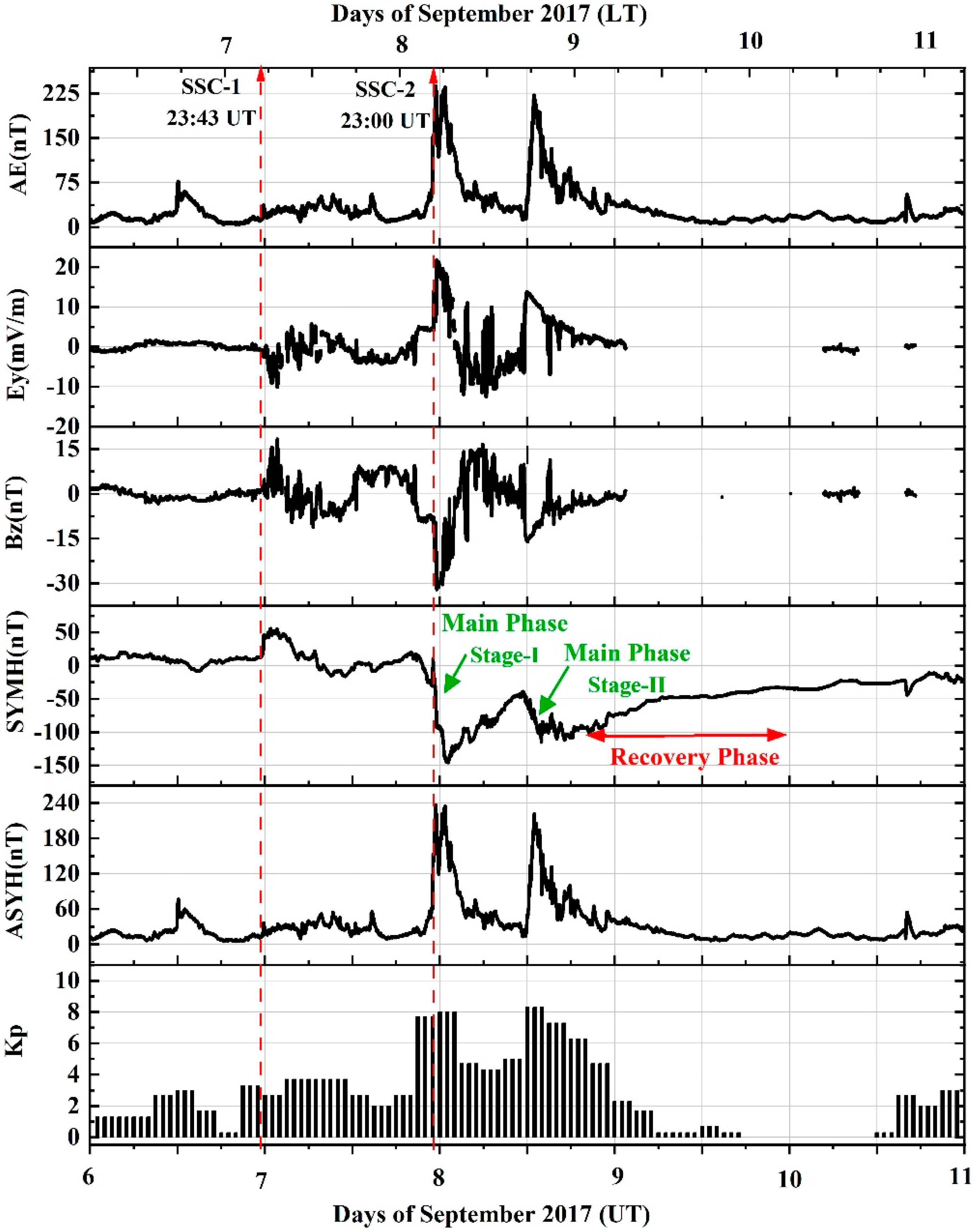
  • The concurrence of ASYH enhancement with the SYMH/local magnetometer H component depressions indicates joule heating at the auroral zone, resulting in the probable DDEF transmission and molecular exchange in conjunction with the PPEF transmission related to magnetospheric convection, making it a complex event in the Indian local time sector.
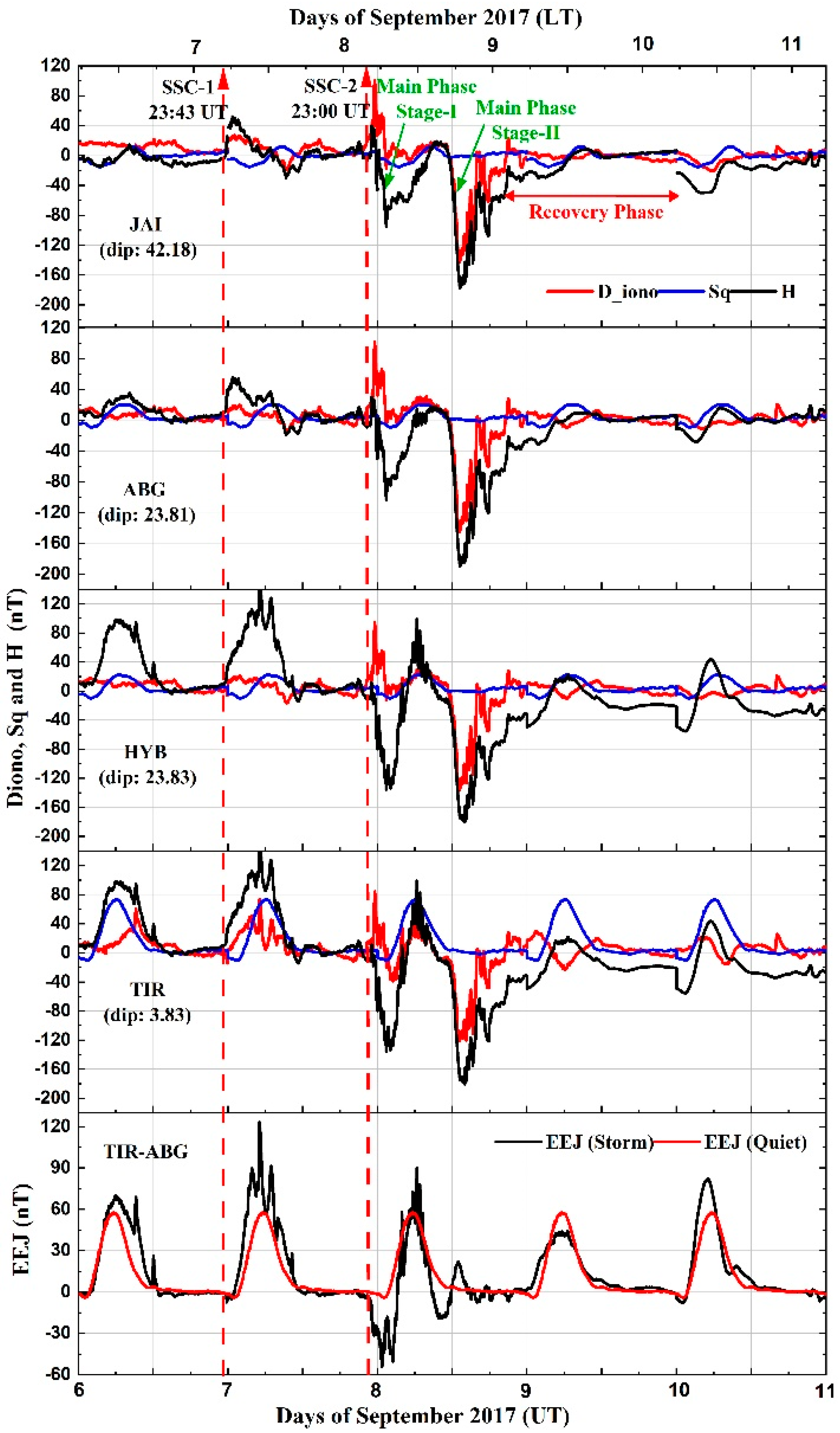
  • The enhanced ASYH signature influenced the local post-midnight to dawn sector, while the large decrease in Diono influenced the daytime ionospheric current during the storm.
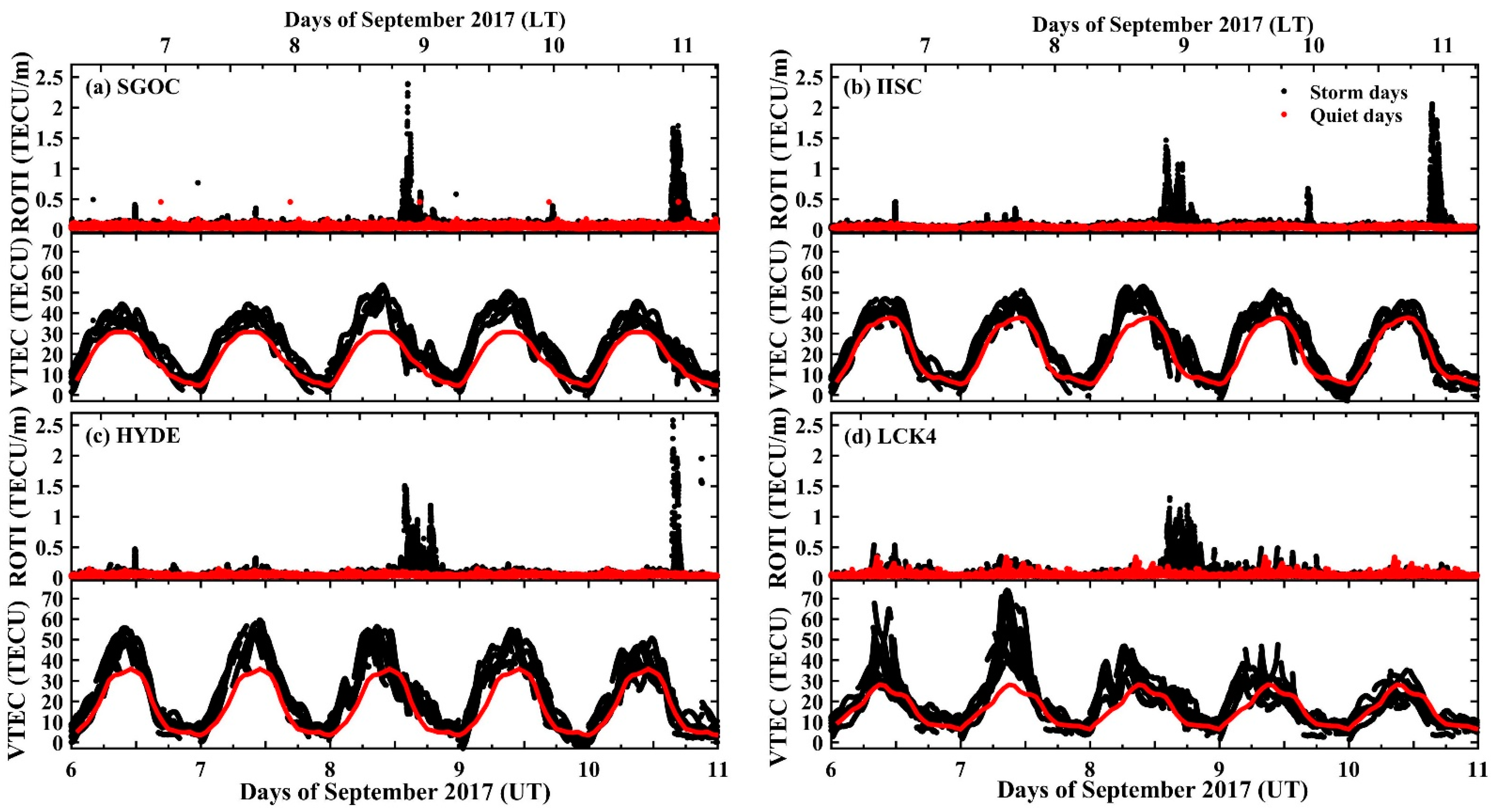
  • The sharp enhancement in the diurnal TEC variations at the higher low-latitude location (LCK4), almost no visible TEC response at the equator (SGOC), and slight enhancements at the intermediate stations (IISC and HYDE) on 7 September are associated with the disturbed equatorial ionization anomaly (EIA), due to multiple M-class flares and prompt penetration electric fields (PPEFs).
  • The significant decrement in the diurnal TEC at the higher low-latitudes and enhancements at the equatorial and nearby sectors on 8 September, confirms the delayed DDEF penetration and reduced EEJ current to suppressed EIA that resulted in the increased ionization over the equator. Additionally, contributions from the storm-time compositional changes (O/N2) in the F-region are also important to characterize the suppressed EIA at low latitudes.
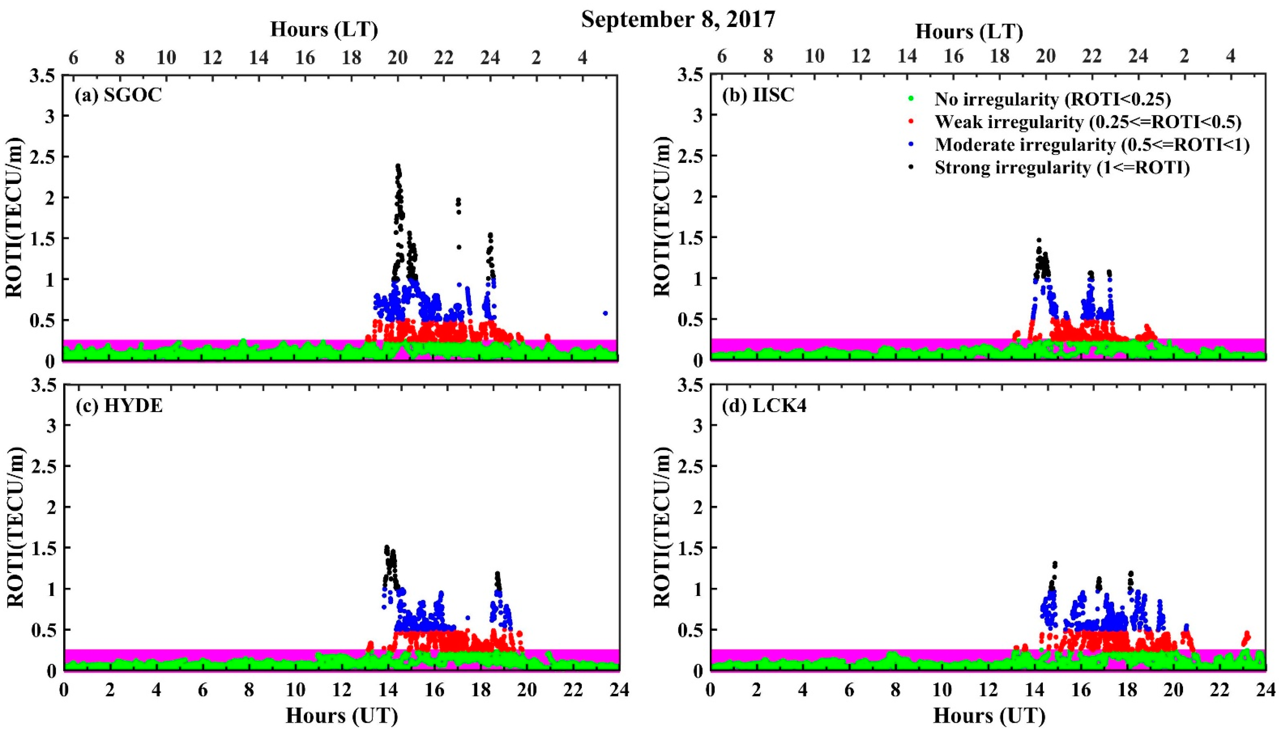
  • On 8 September, the cumulative effects of the southward turning of Bz, the negative departure in SYMH, and the flipped EEJ current conceived a pre-reversal enhancement (PRE)-like scenario. This indeed resulted in a more dominant eastward electric field during the combined effects of PPEF and DDEF during the local evening sector, which was complemented by the penetrating electric field calculations through the real-time PPEFM model. Thus, the PRE seeded the development of the equatorial plasma bubbles (EPBs) in the post-sunset period, which was captured in the ROTI variations at all the stations in our study.
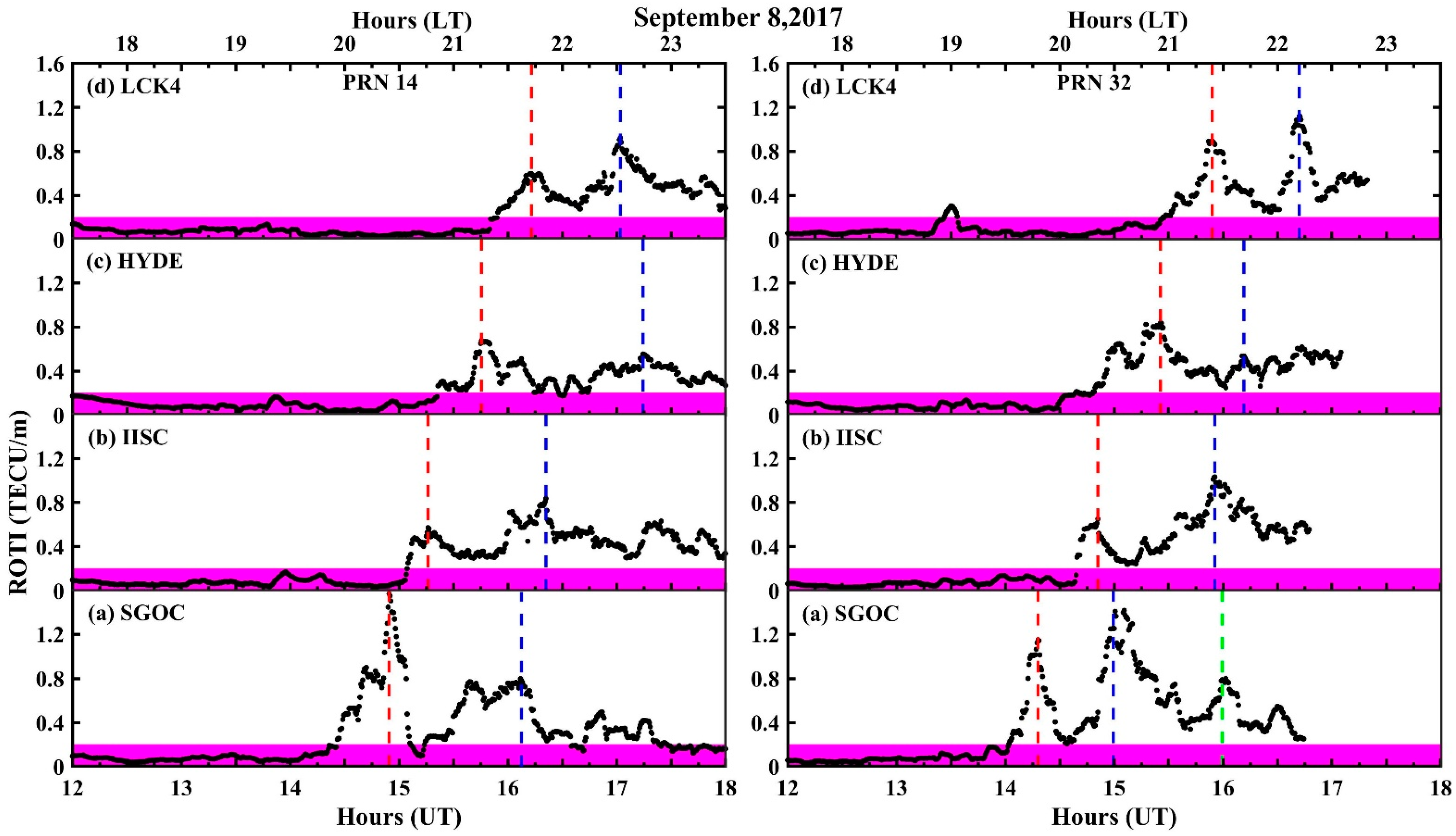
  • The relatively stronger PRE on 8 September caused the EPB to extend more poleward than the movement observed on 10 September, the nearest geomagnetically quiet day.
  • The higher magnitude of ROTI at the equatorial location (SGOC), reaching a level of 2 TECU/min, compared to the other low latitude region, confirms the severity of the scintillations at the equator. This was substantiated from the analysis of the % occurrence rate of the strong, moderate, and weak TEC fluctuations in the ROTI data at the locations.
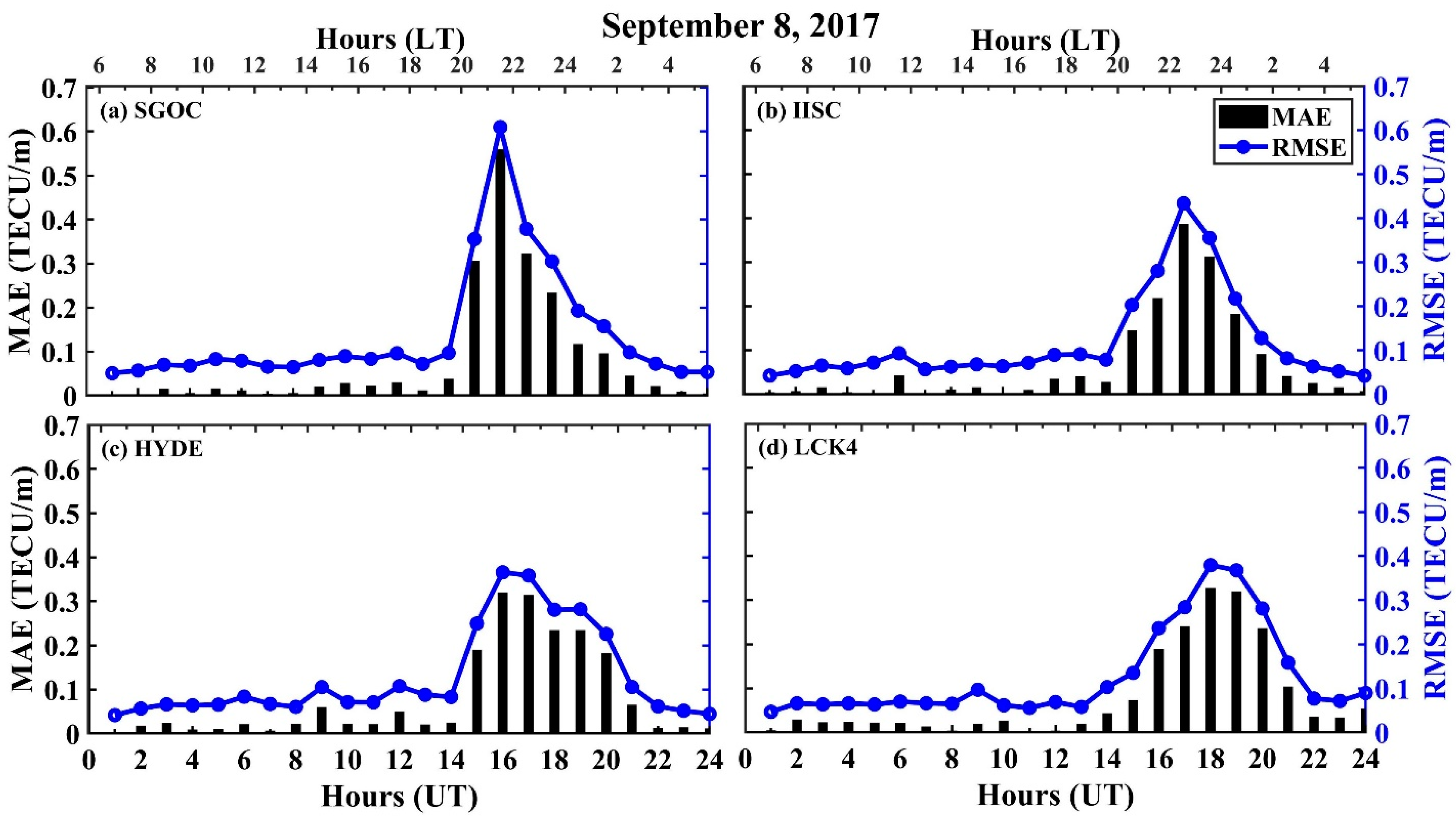
  • Moreover, the largest maximum absolute error (MAE) and root mean square error (RMSE) of ROTI at the equator (SGOC) and its temporal shifts towards higher latitudes suggest the latitudinal movement of irregularities on the day.
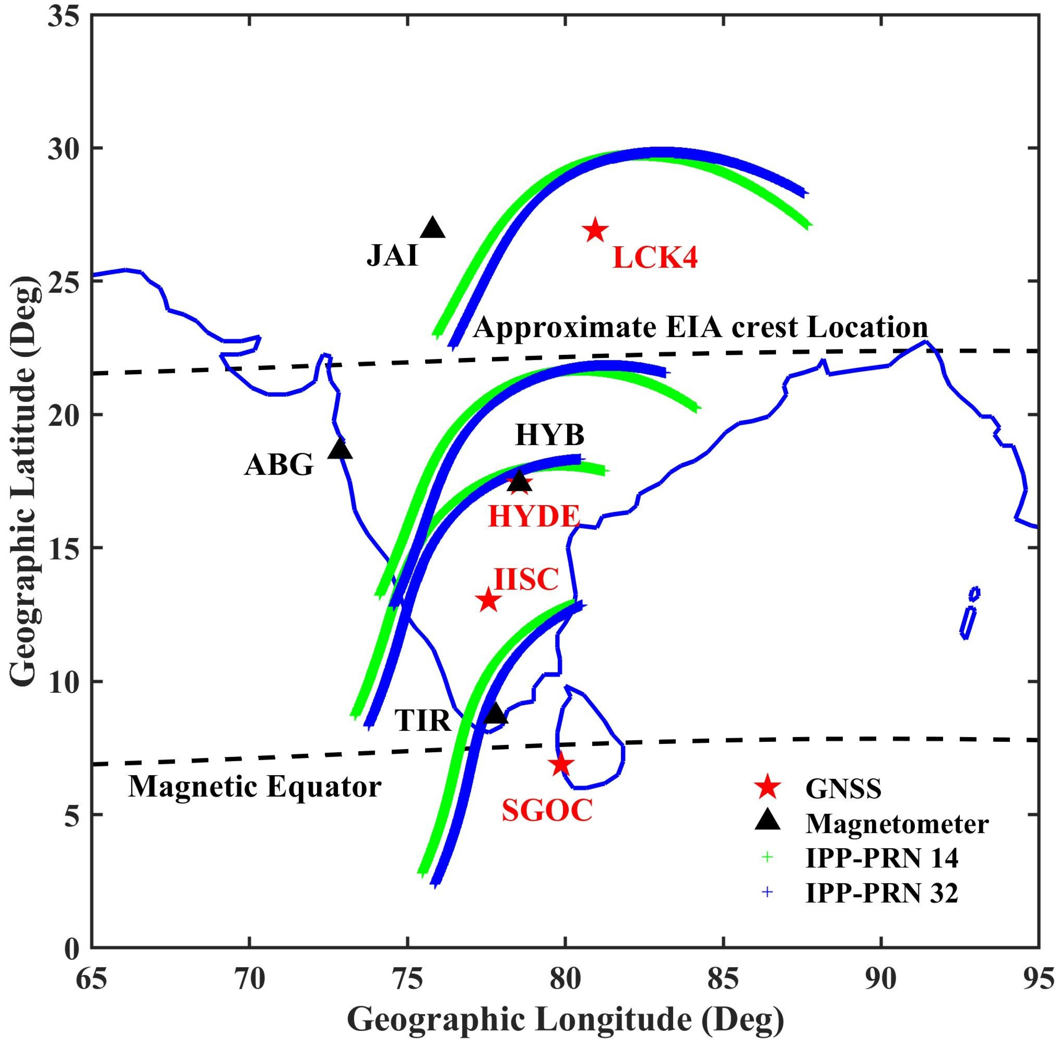
  • The analysis of ROTI variations from two selected GPS PRNs (PRN-14 and PRN-31) suggests the severity of plasma irregularities at the equator and its temporal poleward expansion with a lag between consecutive stations, corroborating the drifting of EPBs towards farther latitudes
In brief, we stress the analysis of the disturbance time ionospheric electric fields/currents from the ground magnetometer observations, along with the TEC and ROTI variations from the standard geodetic GNSS receiver observations, to characterize the evolution and development of the plasma bubbles and their severity on the scintillations to meet the sparse density of the specialized scintillations monitoring the GNSS receivers across the Indian longitude sector. The research is in line with the regional efforts towards exploiting scintillation evolution and mitigations over the equatorial and low latitude Indian region.

Author Contributions

Conceptualization, S.K.P., C.A.-M. and R.F.; methodology, S.K.P. and C.A.-M.; software, R.F., R.K.V., V.R.D., D.O. and M.A.H.; validation, S.K.P., C.A.-M., G.K.S., D.O., T.K.P., M.A.H. and P.J.; formal analysis, S.K.P., C.A.-M., M.A.H., R.K.V. and V.R.D.; investigation, S.K.P., C.A.-M., P.J., T.K.P., R.F. and R.K.V.; resources, S.K.P.; data curation, S.K.P. and G.K.S.; writing—original draft preparation, R.K.V. and S.K.P.; writing—review and editing, S.K.P., V.R.D., C.A.-M., D.O., P.J., T.K.P. and G.K.S.; visualization, S.K.P., V.R.D., C.A.-M., P.J., M.A.H., G.K.S., T.K.P., D.O. and R.F.; supervision, S.K.P.; project administration, S.K.P.; funding acquisition, S.K.P. All authors have read and agreed to the published version of the manuscript.

Funding

This research was funded by the Core Research Grant (CRG) scheme under the Science and Engineering Research Board (SERB) (a statutory body of the Department of Science and Technology, Government of India) New Delhi, India under grant number CRG/2019/003394.

Data Availability Statement

The GNSS observation data used in this study are obtained from the Crustal Dynamics Data Information System (CDDIS) archive (https://cddis.nasa.gov/archive/gnss/, accessed on 6 August 2021). The daily Yuma almanac data required for extracting the TEC and ROTI from the GPS observables are accessed from the United States Coast Guard Navigation Center website (https://www.navcen.uscg.gov/, accessed on 30 July 2021). The authors thank GFZ German Research Centre for Geosciences (ftp://ftp.gfz-potsdam.de, accessed on 9 August 2021) for releasing the international quiet days in each month. The geomagnetic Kp index, interplanetary magnetic field component (IMF-Bz), interplanetary electric field component (Ey), and symmetric H index (SYMH) data are downloaded from the NASA-OMNI website (https://omniweb.gsfc.nasa.gov/, accessed on 8 September 2021). The magnetic field data from Tirunelveli is provided by the Indian Institute of Geomagnetism, whereas that from Alibag, Hyderabad, and Jaipur are downloaded from the INTERMAGNET website (www.intermagnet.org, accessed on 14 October 2021). The penetrating electric field data during the storm period was obtained by running the prompt penetration equatorial electric field model (PPEFM) available at https://geomag.colorado.edu/real-time-model-of-the-ionospheric-electric-fields accessed on 18 January 2022.

Acknowledgments

S.K.P. and R.K.V. acknowledge Koneru Lakshmaiah Education Foundation for providing the necessary laboratory space for conducting this research. S.K.P. sincerely acknowledges S. Sripathi at the Indian Institute of Geomagnetism (IIG), Navi Mumbai, India for the valuable discussion on signatures of PRE in the equatorial ionosonde (CADI) observations at Tirunelveli, India during the storm period of 6–10 September 2017.

Conflicts of Interest

The authors declare no conflict of interest. The funders had no role in the design of the study; in the collection, analyses, or interpretation of data; in the writing of the manuscript; or in the decision to publish the results.

Abbreviations

The following abbreviations are frequently used in this manuscript:
GNSSGlobal Navigation Satellite System
ASYH Asymmetric H index component
SYMHSymmetric H index component
BzInterplanetary magnetic field component
EyInterplanetary electric field component
AEAuroral electrojet index
GPSGlobal Positioning System
TECTotal electron content
EIAEquatorial ionization anomaly
PPEFPrompt penetration electric field
DDEFDisturbance dynamo electric field
EEJEquatorial electrojet
PREPre-reversal enhancement
EPBEquatorial plasma bubble
ROTIRate of change of TEC index
σΦPhase scintillation index
S4Amplitude scintillation index
MAEMaximum absolute error
RMSERoot Mean square error
SRRegular magnetic variation associated with the regular ionospheric dynamo
SqMagnetic field variation due to solar quiet ionospheric current
DionoDisturbance ionospheric current
DP2Disturbance polar current-2
DdynIonospheric disturbed dynamo currents
CMECoronal mass ejection

References

  1. Acharya, R.; Majumdar, S. Statistical relation of scintillation index S4 with ionospheric irregularity index ROTI over Indian equatorial region. Adv. Space Res. 2019, 64, 1019–1033. [Google Scholar] [CrossRef]
  2. Bagiya, M.S.; Thampi, S.V.; Hui, D.; Sunil, A.S.; Chakrabarty, D.; Choudhary, R.K. Signatures of the Solar Transient Disturbances Over the Low Latitude Ionosphere During 6 to 8 September 2017. J. Geophys. Res. Space Phys. 2018, 123, 7598–7608. [Google Scholar] [CrossRef]
  3. Alfonsi, L.; Cesaroni, C.; Spogli, L.; Regi, M.; Paul, A.; Ray, S.; Lepidi, S.; Di Mauro, D.; Haralambous, H.; Oikonomou, C.; et al. Ionospheric Disturbances Over the Indian Sector During 8 September 2017 Geomagnetic Storm: Plasma Structuring and Propagation. Space Weather 2021, 19, e2020SW002607. [Google Scholar] [CrossRef]
  4. Horvath, I.; Lovell, B.C. Magnetosphere-Ionosphere-Thermosphere (M-I-T) Coupling Leading to Equatorial Upward and Westward Drifting Supersonic Plasma Bubble Development and Amplified Subauroral Polarization Streams (SAPS) During the January 21, 2005 Moderate Storm. J. Geophys. Res. Space Phys. 2021, 126, e2020JA028548. [Google Scholar] [CrossRef]
  5. Kelley, M.C.; Fejer, B.G.; Gonzales, C.A. An explanation for anomalous equatorial ionospheric electric fields associated with a northward turning of the interplanetary magnetic field. Geophys. Res. Lett. 1979, 6, 301–304. [Google Scholar] [CrossRef]
  6. Kikuchi, T.; Hashimoto, K.K.; Kitamura, T.; Tachihara, H.; Fejer, B. Equatorial counterelectrojets during substorms. J. Geophys. Res. Earth Surf. 2003, 108, 1406. [Google Scholar] [CrossRef]
  7. Huang, C.-S.; Foster, J.C.; Goncharenko, L.; Reeves, G.; Chau, J.; Yumoto, K.; Kitamura, K. Variations of low-latitude geomagnetic fields andDstindex caused by magnetospheric substorms. J. Geophys. Res. Earth Surf. 2004, 109. [Google Scholar] [CrossRef]
  8. Fejer, B.G.; Navarro, L.A.; Sazykin, S.; Newheart, A.; Milla, M.A.; Condor, P. Prompt Penetration and Substorm Effects Over Jicamarca During the September 2017 Geomagnetic Storm. J. Geophys. Res. Space Phys. 2021, 126, e2021JA029651. [Google Scholar] [CrossRef]
  9. Vasyliunas, V.M. Mathematical Models of Magnetospheric Convection and its Coupling to the Ionosphere. In Particles and Fields in the Magnetosphere; Springer: Dordrecht, The Netherlands, 1970; pp. 60–71. [Google Scholar]
  10. Nishida, A. GeomagneticDp2 fluctuations and associated magnetospheric phenomena. J. Geophys. Res. Earth Surf. 1968, 73, 1795–1803. [Google Scholar] [CrossRef]
  11. Kikuchi, T.; Araki, T.; Maeda, H.; Maekawa, K. Transmission of polar electric fields to the Equator. Nature 1978, 273, 650–651. [Google Scholar] [CrossRef]
  12. Peymirat, C.; Kobea, A.T.; Richmond, A.D. Electrodynamic coupling of high and low latitudes: Simulations of shielding/overshielding effects. J. Geophys. Res. Earth Surf. 2000, 105, 22991–23003. [Google Scholar] [CrossRef]
  13. Blanc, M.; Richmond, A. The ionospheric disturbance dynamo. J. Geophys. Res. Earth Surf. 1980, 85, 1669–1686. [Google Scholar] [CrossRef]
  14. Fejer, B.G.; Larsen, M.F.; Farley, D.T. Equatorial disturbance dynamo electric fields. Geophys. Res. Lett. 1983, 10, 537–540. [Google Scholar] [CrossRef]
  15. Ram, S.T.; Rao, P.V.S.R.; Prasad, D.S.V.V.D.; Niranjan, K.; Krishna, S.G.; Sridharan, R.; Ravindran, S. Local time dependent response of postsunset ESF during geomagnetic storms. J. Geophys. Res. Earth Surf. 2008, 113. [Google Scholar] [CrossRef] [Green Version]
  16. Luo, W.; Xiong, C.; Xu, J.; Zhu, Z.; Chang, S. The Low-Latitude Plasma Irregularities after Sunrise from Multiple Observations in Both Hemispheres during the Recovery Phase of a Storm. Remote Sens. 2020, 12, 2897. [Google Scholar] [CrossRef]
  17. Klobuchar, J.A. Ionospheric Effects on GPS. In Global Positioning System: Theory and Applications; Parkinson, B.W., Spilker, J.J., Eds.; American Institute of Aeronautics & Astronautics: Reston, VA, USA, 1996; Volume 1, pp. 485–515. [Google Scholar]
  18. Klobuchar, J.A.; Doherty, P.H. A Look Ahead: Expected Ionospheric Effects on GPS in 2000. GPS Solut. 1998, 2, 42–48. [Google Scholar] [CrossRef]
  19. Smith, J.; Heelis, R.A. Equatorial plasma bubbles: Variations of occurrence and spatial scale in local time, longitude, season, and solar activity. J. Geophys. Res. Space Phys. 2017, 122, 5743–5755. [Google Scholar] [CrossRef]
  20. Okoh, D.; Rabiu, B.; Shiokawa, K.; Otsuka, Y.; Segun, B.; Falayi, E.; Onwuneme, S.; Kaka, R. First Study on the Occurrence Frequency of Equatorial Plasma Bubbles over West Africa Using an All-Sky Airglow Imager and GNSS Receivers. J. Geophys. Res. Space Phys. 2017, 122, 12–430. [Google Scholar] [CrossRef]
  21. Gurav, O.; Sripathi, S.; Ghodpage, R. Radio and optical investigations of storm time evolution of post-midnight equatorial plasma bubbles (EPBs) and their drifts over Indian sector. Adv. Space Res. 2021, 67, 87–101. [Google Scholar] [CrossRef]
  22. Joshi, L.M.; Patra, A.K.; Pant, T.K.; Rao, S.V.B. On the nature of low-latitudeEsinfluencing the genesis of equatorial plasma bubble. J. Geophys. Res. Space Phys. 2013, 118, 524–532. [Google Scholar] [CrossRef] [Green Version]
  23. Seif, A.; Tsunoda, R.T.; Abdullah, M.; Hasbi, A.M. Daytime gigahertz scintillations near magnetic equator: Relationship to blanketing sporadic E and gradient-drift instability. Earth Planets Space 2015, 67, 177. [Google Scholar] [CrossRef] [Green Version]
  24. Bhattacharyya, A.; Beach, T.L.; Basu, S.; Kintner, P.M. Nighttime equatorial ionosphere: GPS scintillations and differential carrier phase fluctuations. Radio Sci. 2000, 35, 209–224. [Google Scholar] [CrossRef]
  25. Luo, X.; Gu, S.; Lou, Y.; Cai, L.; Liu, Z. Amplitude scintillation index derived from C/N0 measurements released by common geodetic GNSS receivers operating at 1 Hz. J. Geodesy 2020, 94, 27. [Google Scholar] [CrossRef]
  26. Goodman, J.L.; Kramer, L. Scintillation Effects on Space Shuttle GPS Data. In Proceedings of the 2001 National Technical Meeting of The Institute of Navigation, Long Beach, CA, USA, 22–24 January 2001; pp. 742–752. [Google Scholar]
  27. Bolaji, O.; Adebiyi, S.; Fashae, J. Characterization of ionospheric irregularities at different longitudes during quiet and disturbed geomagnetic conditions. J. Atmos. Sol.-Terr. Phys. 2019, 182, 93–100. [Google Scholar] [CrossRef] [Green Version]
  28. Pi, X.; Mannucci, A.J.; Lindqwister, U.J.; Ho, C.M. Monitoring of global ionospheric irregularities using the Worldwide GPS Network. Geophys. Res. Lett. 1997, 24, 2283–2286. [Google Scholar] [CrossRef]
  29. Olwendo, J.O.; Cilliers, P.; Weimin, Z.; Ming, O.; Yu, X. Validation of ROTI for Ionospheric Amplitude Scintillation Measurements in a Low-Latitude Region Over Africa. Radio Sci. 2018, 53, 876–887. [Google Scholar] [CrossRef]
  30. Li, C.; Hancock, C.M.; Hamm, N.A.S.; Veettil, S.V.; You, C. Analysis of the Relationship between Scintillation Parameters, Multipath and ROTI. Sensors 2020, 20, 2877. [Google Scholar] [CrossRef]
  31. Gogie, T.K. The Rate of Ionospheric Total Electron Content Index (ROTI) as a Proxy for Nighttime Ionospheric Irregularity Using Ethiopian Low-Latitude GPS Data. Geomagn. Aeron. 2021, 61, 464–475. [Google Scholar] [CrossRef]
  32. Kotulak, K.; Zakharenkova, I.; Krankowski, A.; Cherniak, I.; Wang, N.; Fron, A. Climatology Characteristics of Ionospheric Irregularities Described with GNSS ROTI. Remote Sens. 2020, 12, 2634. [Google Scholar] [CrossRef]
  33. Carmo, C.S.; Denardini, C.M.; Figueiredo, C.A.O.B.; Resende, L.C.A.; Picanço, G.A.S.; Neto, P.F.B.; Nogueira, P.A.B.; Moro, J.; Chen, S.S. Evaluation of Different Methods for Calculating the ROTI Index Over the Brazilian Sector. Radio Sci. 2021, 56, e2020RS007140. [Google Scholar] [CrossRef]
  34. Cherniak, I.; Krankowski, A.; Zakharenkova, I. ROTI Maps: A new IGS ionospheric product characterizing the ionospheric irregularities occurrence. GPS Solutions 2018, 22, 69. [Google Scholar] [CrossRef]
  35. Raghunath, S.; Venkata Ratnam, D. Detection of Ionospheric Spatial and Temporal Gradients for Ground Based Augmentation System Applications. Indian J. Radio Space Phys. 2016, 45, 11–19. [Google Scholar]
  36. Harsha, P.B.S.; Ratnam, D.V.; Nagasri, M.L.; Sridhar, M.; Raju, K.P. Kriging-Based Ionospheric TEC, ROTI and Amplitude Scintillation Index (S 4) Maps for India. IET Radar Sonar Navig. 2020, 14, 1827–1836. [Google Scholar] [CrossRef]
  37. Li, Q.; Zhu, Y.; Fang, K.; Fang, J. Statistical Study of the Seasonal Variations in TEC Depletion and the ROTI during 2013–2019 over Hong Kong. Sensors 2020, 20, 6200. [Google Scholar] [CrossRef] [PubMed]
  38. Manga, N.A.; Lakshmanna, K.; Sarma, A.D.; Pant, T.K. Analysis of Correlation between Roti and S4 Using Gagan Data. Prog. Electromagn. Res. M 2021, 99, 23–34. [Google Scholar] [CrossRef]
  39. Yang, Z.; Liu, Z. Correlation between ROTI and Ionospheric Scintillation Indices using Hong Kong low-latitude GPS data. GPS Solutions 2016, 20, 815–824. [Google Scholar] [CrossRef]
  40. Xiong, B.; Wan, W.-X.; Ning, B.-Q.; Yuan, H.; Li, G.-Z. A Comparison and Analysis of theS4Index, C/N and Roti over Sanya. Chin. J. Geophys. 2007, 50, 1414–1424. [Google Scholar] [CrossRef]
  41. Kumar, S. Morphology of equatorial plasma bubbles during low and high solar activity years over Indian sector. Astrophys. Space Sci. 2017, 362, 93. [Google Scholar] [CrossRef]
  42. Bagiya, M.S.; Iyer, K.N.; Joshi, H.; Thampi, S.V.; Tsugawa, T.; Ravindran, S.; Sridharan, R.; Pathan, B.M. Low-latitude ionospheric-thermospheric response to storm time electrodynamical coupling between high and low latitudes. J. Geophys. Res. Earth Surf. 2011, 116. [Google Scholar] [CrossRef] [Green Version]
  43. Srinivasu, V.; Prasad, D.; Niranjan, K.; Seemala, G.K.; Venkatesh, K. L-Band Scintillation and TEC Variations on St. Patrick’s Day Storm of 17 March 2015 over Indian Longitudes Using GPS and GLONASS Observations. J. Earth Syst. Sci. 2019, 128, 69. [Google Scholar] [CrossRef] [Green Version]
  44. Aa, E.; Huang, W.; Liu, S.; Ridley, A.; Zou, S.; Shi, L.; Chen, Y.; Shen, H.; Yuan, T.; Li, J.; et al. Midlatitude Plasma Bubbles Over China and Adjacent Areas During a Magnetic Storm on 8 September 2017. Space Weather 2018, 16, 321–331. [Google Scholar] [CrossRef]
  45. Zhang, R.; Liu, L.; Le, H.; Chen, Y. Equatorial Ionospheric Electrodynamics Over Jicamarca During the 6–11 September 2017 Space Weather Event. J. Geophys. Res. Space Phys. 2019, 124, 1292–1306. [Google Scholar] [CrossRef]
  46. Lei, J.; Huang, F.; Chen, X.; Zhong, J.; Ren, D.; Wang, W.; Yue, X.; Luan, X.; Jia, M.; Dou, X.; et al. Was Magnetic Storm the Only Driver of the Long-Duration Enhancements of Daytime Total Electron Content in the Asian-Australian Sector Between 7 and 12 September 2017? J. Geophys. Res. Space Phys. 2018, 123, 3217–3232. [Google Scholar] [CrossRef]
  47. Li, G.; Ning, B.; Wang, C.; Abdu, M.A.; Otsuka, Y.; Yamamoto, M.; Wu, J.; Chen, J. Storm-Enhanced Development of Postsunset Equatorial Plasma Bubbles Around the Meridian 120°E/60°W on 7-8 September 2017. J. Geophys. Res. Space Phys. 2018, 123, 7985–7998. [Google Scholar] [CrossRef]
  48. Nishimura, Y.; Mrak, S.; Semeter, J.L.; Coster, A.J.; Jayachandran, P.T.; Groves, K.M.; Knudsen, D.J.; Nishitani, N.; Ruohoniemi, J.M. Evolution of Mid-latitude Density Irregularities and Scintillation in North America During the 7–8 September 2017 Storm. J. Geophys. Res. Space Phys. 2021, 126, e2021JA029192. [Google Scholar] [CrossRef]
  49. Wei, L.; Jiang, C.; Hu, Y.; Aa, E.; Huang, W.; Liu, J.; Yang, G.; Zhao, Z. Ionosonde Observations of Spread F and Spread Es at Low and Middle Latitudes during the Recovery Phase of the 7–9 September 2017 Geomagnetic Storm. Remote Sens. 2021, 13, 1010. [Google Scholar] [CrossRef]
  50. Jimoh, O.; Lei, J.; Zhong, J.; Owolabi, C.; Luan, X.; Dou, X. Topside Ionospheric Conditions During the 7–8 September 2017 Geomagnetic Storm. J. Geophys. Res. Space Phys. 2019, 124, 9381–9404. [Google Scholar] [CrossRef]
  51. De Paula, E.R.; de Oliveira, C.M.; Caton, R.G.; Negreti, P.M.; Batista, I.S.; Martinon, A.R.F.; Neto, A.C.; Abdu, M.A.; Monico, J.F.G.; Sousasantos, J.; et al. Ionospheric irregularity behavior during the September 6–10, 2017 magnetic storm over Brazilian equatorial–low latitudes. Earth Planets Space 2019, 71, 42. [Google Scholar] [CrossRef]
  52. Aa, E.; Zou, S.; Ridley, A.; Zhang, S.; Coster, A.J.; Erickson, P.J.; Liu, S.; Ren, J. Merging of Storm Time Midlatitude Traveling Ionospheric Disturbances and Equatorial Plasma Bubbles. Space Weather 2019, 17, 285–298. [Google Scholar] [CrossRef]
  53. Nair, K.N.; Rastogi, R.G.; Sarabhai, V.; Nair, R.G.R.K.N. Daily Variation of the Geomagnetic Field at the Dip Equator. Nature 1970, 226, 740–741. [Google Scholar] [CrossRef] [PubMed]
  54. Bhaskar, A.; Vichare, G. Characteristics of penetration electric fields to the equatorial ionosphere during southward and northward IMF turnings. J. Geophys. Res. Space Phys. 2013, 118, 4696–4709. [Google Scholar] [CrossRef]
  55. Panda, S.; Gedam, S.; Rajaram, G.; Sripathi, S.; Bhaskar, A. Impact of the 15 January 2010 annular solar eclipse on the equatorial and low latitude ionosphere over the Indian region. J. Atmos. Sol.-Terr. Phys. 2015, 135, 181–191. [Google Scholar] [CrossRef] [Green Version]
  56. Shao, X.; Guzdar, P.N.; Milikh, G.M.; Papadopoulos, K.; Goodrich, C.C.; Sharma, A.; Wiltberger, M.J.; Lyon, J.G. Comparing ground magnetic field perturbations from global MHD simulations with magnetometer data for the 10 January 1997 magnetic storm event. J. Geophys. Res. Earth Surf. 2002, 107, SMP11. [Google Scholar] [CrossRef] [Green Version]
  57. Huy, M.L.; Amory-Mazaudier, C. Magnetic signature of the ionospheric disturbance dynamo at equatorial latitudes: “Ddyn”. J. Geophys. Res. Earth Surf. 2005, 110. [Google Scholar] [CrossRef]
  58. Nava, B.; Rodríguez-Zuluaga, J.; Alazo-Cuartas, K.; Kashcheyev, A.; Migoya-Orué, Y.; Radicella, S.; Amory-Mazaudier, C.; Fleury, R. Middle- and low-latitude ionosphere response to 2015 St. Patrick’s Day geomagnetic storm. J. Geophys. Res. Space Phys. 2016, 121, 3421–3438. [Google Scholar] [CrossRef] [Green Version]
  59. Kashcheyev, A.; Migoya-Orue, Y.; Amory-Mazaudier, C.; Fleury, R.; Nava, B.; Alazo-Cuartas, K.; Radicella, S.M. Multivariable Comprehensive Analysis of Two Great Geomagnetic Storms of 2015. J. Geophys. Res. Space Phys. 2018, 123, 5000–5018. [Google Scholar] [CrossRef]
  60. Imtiaz, N.; Younas, W.; Khan, M. Response of the low- to mid-latitude ionosphere to the geomagnetic storm of September 2017. Ann. Geophys. 2020, 38, 359–372. [Google Scholar] [CrossRef] [Green Version]
  61. Amaechi, P.O.; Oyeyemi, E.O.; Akala, A.O.; Amory-Mazaudier, C. Geomagnetic Activity Control of Irregularities Occurrences Over the Crests of the African EIA. Earth Space Sci. 2020, 7, e2020EA001183. [Google Scholar] [CrossRef]
  62. Younas, W.; Amory-Mazaudier, C.; Khan, M.; Fleury, R. Ionospheric and Magnetic Signatures of a Space Weather Event on 25–29 August 2018: CME and HSSWs. J. Geophys. Res. Space Phys. 2020, 125, e2020JA027981. [Google Scholar] [CrossRef]
  63. Fuller-Rowell, T.J.; Codrescu, M.V.; Moffett, R.J.; Quegan, S. Response of the thermosphere and ionosphere to geomagnetic storms. J. Geophys. Res. Earth Surf. 1994, 99, 3893–3914. [Google Scholar] [CrossRef]
  64. Reddybattula, K.D.; Panda, S.K.; Sharma, S.K.; Singh, A.K.; Kurnala, K.; Haritha, C.S.; Wuyyuru, S. Anomaly effects of 6–10 September 2017 solar flares on ionospheric total electron content over Saudi Arabian low latitudes. Acta Astronaut. 2020, 177, 332–340. [Google Scholar] [CrossRef]
  65. Jenan, R.; Dammalage, T.L.; Panda, S.K. Ionospheric total electron content response to September-2017 geomagnetic storm and December-2019 annular solar eclipse over Sri Lankan region. Acta Astronaut. 2021, 180, 575–587. [Google Scholar] [CrossRef]
  66. Roble, R.G.; Dickinson, R.E.; Ridley, E.C. Seasonal and solar cycle variations of the zonal mean circulation in the thermosphere. J. Geophys. Res. Earth Surf. 1977, 82, 5493–5504. [Google Scholar] [CrossRef]
  67. Prölss, G.W. Magnetic storm associated perturbations of the upper atmosphere: Recent results obtained by satellite-borne gas analyzers. Rev. Geophys. 1980, 18, 183–202. [Google Scholar] [CrossRef]
  68. Burns, A.G.; Killeen, T.L.; Roble, R.G. A theoretical study of thermospheric composition perturbations during an impulsive geomagnetic storm. J. Geophys. Res. Earth Surf. 1991, 96, 14153–14167. [Google Scholar] [CrossRef]
  69. Liou, K.; Newell, P.T.; Anderson, B.J.; Zanetti, L.; Meng, C. Neutral composition effects on ionospheric storms at middle and low latitudes. J. Geophys. Res. Earth Surf. 2005, 110. [Google Scholar] [CrossRef] [Green Version]
  70. Liemohn, M.; Kozyra, J.U.; Thomsen, M.F.; Roeder, J.L.; Lu, G.; Borovsky, J.E.; Cayton, T.E. Dominant role of the asymmetric ring current in producing the stormtimeDst*. J. Geophys. Res. Earth Surf. 2001, 106, 10883–10904. [Google Scholar] [CrossRef] [Green Version]
  71. Ram, S.T.; Yokoyama, T.; Otsuka, Y.; Shiokawa, K.; Sripathi, S.; Veenadhari, B.; Heelis, R.; Ajith, K.K.; Gowtam, V.S.; Gurubaran, S.; et al. Duskside enhancement of equatorial zonal electric field response to convection electric fields during the St. Patrick’s Day storm on 17 March 2015. J. Geophys. Res. Space Phys. 2015, 121, 538–548. [Google Scholar] [CrossRef]
  72. Abdu, M.A.; Nogueira, P.A.B.; Santos, A.M.; De Souza, J.R.; Batista, I.S.; Sobral, J.H.A. Impact of disturbance electric fields in the evening on prereversal vertical drift and spread F developments in the equatorial ionosphere. Ann. Geophys. 2018, 36, 609–620. [Google Scholar] [CrossRef]
  73. Rishbeth, H. The F-layer dynamo. Planet. Space Sci. 1971, 19, 263–267. [Google Scholar] [CrossRef]
  74. Rishbeth, H. Polarization fields produced by winds in the equatorial F-region. Planet. Space Sci. 1971, 19, 357–369. [Google Scholar] [CrossRef]
  75. Farley, D.T.; Bonelli, E.; Fejer, B.G.; Larsen, M.F. The prereversal enhancement of the zonal electric field in the equatorial ionosphere. J. Geophys. Res. Earth Surf. 1986, 91, 13723–13728. [Google Scholar] [CrossRef]
  76. Eccles, J.V.; Maurice, J.P.S.; Schunk, R.W. Mechanisms underlying the prereversal enhancement of the vertical plasma drift in the low-latitude ionosphere. J. Geophys. Res. Space Phys. 2015, 120, 4950–4970. [Google Scholar] [CrossRef] [Green Version]
  77. Abadi, P.; Otsuka, Y.; Liu, H.; Hozumi, K.; Martinigrum, D.R.; Jamjareegulgarn, P.; Thanh, L.T.; Otadoy, R. Roles of thermospheric neutral wind and equatorial electrojet in pre-reversal enhancement, deduced from observations in Southeast Asia. Earth Planet. Phys. 2021, 5, 388–397. [Google Scholar] [CrossRef]
  78. Manoj, C.; Maus, S. A real-time forecast service for the ionospheric equatorial zonal electric field. Space Weather 2012, 10. [Google Scholar] [CrossRef]
  79. Nayak, C.; Tsai, L.-C.; Su, S.-Y.; Galkin, I.; Caton, R.; Groves, K. Suppression of ionospheric scintillation during St. Patrick’s Day geomagnetic super storm as observed over the anomaly crest region station Pingtung, Taiwan: A case study. Adv. Space Res. 2017, 60, 396–405. [Google Scholar] [CrossRef]
  80. Dugassa, T.; Habarulema, J.B.; Nigussie, M. Longitudinal variability of occurrence of ionospheric irregularities over the American, African and Indian regions during geomagnetic storms. Adv. Space Res. 2019, 63, 2609–2622. [Google Scholar] [CrossRef]
  81. Habarulema, J.B.; Katamzi-Joseph, Z.T.; Burešová, D.; Nndanganeni, R.; Matamba, T.; Tshisaphungo, M.; Buchert, S.; Kosch, M.; Lotz, S.; Cilliers, P.; et al. Ionospheric Response at Conjugate Locations During the 7–8 September 2017 Geomagnetic Storm Over the Europe-African Longitude Sector. J. Geophys. Res. Space Phys. 2020, 125. [Google Scholar] [CrossRef]
  82. Navarro, L.A.; Fejer, B.G.; Scherliess, L. Equatorial Disturbance Dynamo Vertical Plasma Drifts Over Jicamarca: Bimonthly and Solar Cycle Dependence. J. Geophys. Res. Space Phys. 2019, 124, 4833–4841. [Google Scholar] [CrossRef] [Green Version]
  83. Chakraborty, M.; Singh, A.; Rao, S. Solar flares and geomagnetic storms of September 2017: Their impacts on the TEC over 75°E longitude sector. Adv. Space Res. 2021, 68, 1825–1835. [Google Scholar] [CrossRef]
  84. Valladares, C.E.; Villalobos, J.; Sheehan, R.; Hagan, M.P. Latitudinal extension of low-latitude scintillations measured with a network of GPS receivers. Ann. Geophys. 2004, 22, 3155–3175. [Google Scholar] [CrossRef]
  85. Abadi, P.; Otsuka, Y.; Tsugawa, T. Effects of pre-reversal enhancement of E × B drift on the latitudinal extension of plasma bubble in Southeast Asia. Earth Planets Space 2015, 67, 74. [Google Scholar] [CrossRef] [Green Version]
  86. Liu, X.; Yuan, Y.; Tan, B.; Li, M. Observational Analysis of Variation Characteristics of GPS-Based TEC Fluctuation over China. ISPRS Int. J. Geo-Inf. 2016, 5, 237. [Google Scholar] [CrossRef] [Green Version]
  87. Alfonsi, L.; Spogli, L.; Tong, J.; De Franceschi, G.; Romano, V.; Bourdillon, A.; Le Huy, M.; Mitchell, C. GPS scintillation and TEC gradients at equatorial latitudes in April 2006. Adv. Space Res. 2011, 47, 1750–1757. [Google Scholar] [CrossRef]
  88. Basu, S.; Groves, K.; Quinn, J.; Doherty, P. A comparison of TEC fluctuations and scintillations at Ascension Island. J. Atmospheric Sol.-Terr. Phys. 1999, 61, 1219–1226. [Google Scholar] [CrossRef]
  89. Jacobsen, K.S.; Dähnn, M. Statistics of ionospheric disturbances and their correlation with GNSS positioning errors at high latitudes. J. Space Weather Space Clim. 2014, 4, A27. [Google Scholar] [CrossRef] [Green Version]
  90. Carrano, C.S.; Groves, K.M.; Rino, C.L. On the Relationship Between the Rate of Change of Total Electron Content Index (ROTI), Irregularity Strength (CkL), and the Scintillation Index (S4). J. Geophys. Res. Space Phys. 2019, 124, 2099–2112. [Google Scholar] [CrossRef]
  91. Aquino, M.; Moore, T.; Dodson, A.; Waugh, S.; Souter, J.; Rodrigues, F.S. Implications of Ionospheric Scintillation for GNSS Users in Northern Europe. J. Navig. 2005, 58, 241–256. [Google Scholar] [CrossRef]
  92. Nguyen, C.T.; Oluwadare, S.T.; Le, N.T.; Alizadeh, M.; Wickert, J.; Schuh, H. Spatial and Temporal Distributions of Ionospheric Irregularities Derived from Regional and Global ROTI Maps. Remote Sens. 2021, 14, 10. [Google Scholar] [CrossRef]
  93. Abdu, M.A.; De Medeiros, R.T.; Sobral, J.H.A.; Bittencourt, J.A. Spread F plasma bubble vertical rise velocities determined from spaced ionosonde observations. J. Geophys. Res. Earth Surf. 1983, 88, 9197–9204. [Google Scholar] [CrossRef]
  94. Dabas, R.S.; Reddy, B.M. Equatorial plasma bubble rise velocities in the Indian sector determined from multistation scintillation observations. Radio Sci. 1990, 25, 125–132. [Google Scholar] [CrossRef]
  95. Huang, Y.-N. Drift motion of ionospheric bubbles at the equatorial anomaly crest region. J. Geophys. Res. Earth Surf. 1990, 95, 4297. [Google Scholar] [CrossRef]
  96. Sun, L.; Xu, J.; Zhu, Y.; Yuan, W.; Chen, Z.; Hao, Y.; Hu, L.; Zhang, D.; Guo, B.; Zhao, X. Interaction Between a Southwestward Propagating MSTID and a Poleward Moving WSA-Like Plasma Patch on a Magnetically Quiet Night at Midlatitude China Region. J. Geophys. Res. Space Phys. 2020, 125, e2020JA028085. [Google Scholar] [CrossRef]
Figure 1. Geographic locations of the magnetometer observatories (black triangle) and the IGS GNSS stations (red star) in the Indian longitude sector considered in the study. The dashed horizontal contour lines represent the approximate positions of the magnetic equator and northern EIA crest. The ionospheric piercing point (IPP) locations for the GPS PRNs, 14 and 32, during the storm on 8 September 2017 are indicated by the green (+) and blue (+) curves, respectively.
Remotesensing 14 00652 g001
Figure 2. Variation of the Kp, ASYH, SYMH, Bz, Ey, and AE indices during the geomagnetic storm period from 6–10 September 2017, arranged from the bottom to the top panel. The arrow-headed, vertical, red, dashed lines indicate the SSCs due to the shocks of the coronal mass ejections (CMEs). The storm main phase stage-I and stage-II as well as the recovery phase are indicated in the Figure.
Remotesensing 14 00652 g002
Figure 3. Variation of the horizontal magnetic field component H (in black), superimposed with the regular Sq variation (in blue) and Diono component (in red) that corresponds to the disturbances due to ionospheric currents registered at all four magnetometer observatories (top 4-panels) during the storm period from 6–10 September 2017. The bottom panel shows the variation of the EEJ proxy index during the storm period (in black) superimposed with the averaged quiet-time reference level (in red).
Remotesensing 14 00652 g003
Figure 4. Effects of the prompt penetration electric fields (PPEFs) towards the enhanced duskside PRF calculated from the real-time prompt penetration electric field model (PPEFM; https://geomag.colorado.edu/real-time-model-of-the-ionospheric-electric-fields, accessed on 18 January 2022) [78] over the Indian longitude (78° E) in the main phase of the storm during 6–10 September 2017. The black line shows the background quiet-time electric field, whereas the blue and red lines indicate the prompt penetration electric field and the total electric field (the sum of quiet-time and prompt penetration electric fields), respectively.
Remotesensing 14 00652 g004
Figure 5. Variation of the VTEC and ROTI parameters at (a) SGOC, Colombo; (b) IISC, Bangalore; (c) HYDE, Hyderabad; and (d) LCK4, Lucknow, during the storm period from 6–10 September 2017 (in black), superimposed with the corresponding quiet-time reference values (in red).
Remotesensing 14 00652 g005
Figure 6. Classification of the ionospheric irregularities based on the ROTI values at (a) SGOC, Colombo, (b) IISC, Bangalore, (c) HYDE, Hyderabad, and (d) LCK4, Lucknow on the geomagnetic storm day (8 September 2017). The criteria for the classification of the irregularities is chosen as (i) no irregularity (ROTI < 0.25; in green); (ii) weak irregularity (0.25 ≤ ROTI < 0.5; in red); (iii) moderate irregularity (0.5 ≤ ROTI < 1; in blue); and (iv) strong irregularity (ROTI ≥ 1; black). The shaded portion with ROTI < 0.25 is masked out in this study.
Remotesensing 14 00652 g006
Figure 7. Diurnal maximum absolute error (MAE) and root mean square error (RMSE) of ROTI at (a) SGOC, Colombo, (b) IISC, Bangalore, (c) HYDE, Hyderabad, and (d) LCK4, Lucknow on the geomagnetic storm day (8 September 2017), with respect to the averaged quiet-time reference level.
Remotesensing 14 00652 g007
Figure 8. Spatiotemporal variation of the plasma irregularities marked from the simultaneous ROTI observations from PRN-14 and PRN-32 GPS satellite signals at (a) SGOC, Colombo, (b) IISC, Bangalore, (c) HYDE, Hyderabad, and (d) LCK4, Lucknow on the geomagnetic storm day (8 September 2017), respectively arranged from bottom to top. The vertical dotted lines indicate the timestamps of corresponding ROTI peaks at all stations. The pink-colored shaded portion at the bottom indicates the masked-out ROTI values (ROTI < 0.25), wherein the TEC fluctuation is assumed to be absent.
Remotesensing 14 00652 g008
Table 1. The geographic and geomagnetic coordinates of the considered magnetometer observatories and IGS GNSS stations, along with their respective magnetic dips considered in this study.
SchemeStation CodeGeog.
Latitude
Geog.
Longitude
Geomag.
Latitude
Geomag. LongitudeMagnetic DipObservation
Type
Jaipur, IndiaJAI26.91°N75.80°E18.5°N150.47°E42.18°Magnetometer
Lucknow, IndiaLCK426.90°N80.95°E18.1°N155.30°E42.09°GNSS
Alibag, IndiaABG18.62°N72.87°E10.54°N146.89°E26.81°Magnetometer
Hyderabad, IndiaHYDE17.42°N78.55°E8.87°N152.25°E23.96°GNSS
Hyderabad, IndiaHYB17.41°N78.55°E8.87°N152.25°E23.94°Magnetometer
Bangalore, IndiaIISC13.03°N77.57°E4.61°N150.87°E14.10°GNSS
Tirunelveli, IndiaTIR8.70°N77.80°E0.29°N150.81°E3.82°Magnetometer
Colombo, Sri Lanka.SGOC6.88°N79.87°E1.66°S152.71°E4.2°GNSS
Table 2. Increased and decreased levels of Diono and their corresponding local time (LT) on the geomagnetic storm day (8 September 2017).
SchemeLT–UT DipMain Phase Stage-IMain Phase Stage-II
(HH:MM)Diono
(Increase)
LT (HH:MM)Diono
(Decrease)
LT (HH:MM)
JAI05:0342.18°100.03 nT04:27−141.66 nT18:15
ABG04:5126.81°101.66 nT04:15−145.52 nT18:03
HYB05:1423.82°94.65 nT04:38−135.93 nT18:26
TIR05:113.82°84.35 nT04:35−121.07 nT18:23
Table 3. Percentage occurrence rate of strong, moderate, and weak ionospheric irregularities at (a) SGOC, Colombo, (b) IISC, Bangalore, (c) HYDE, Hyderabad, and (d) LCK4, Lucknow on the geomagnetic storm day (8 September 2017).
GNSS Station
Code
Magnetic
Dip
(In Degrees)
Strong
Irregularities
(% Occurrence Rate)
Moderate
Irregularities
(% Occurrence Rate)
Weak
Irregularities
(% Occurrence Rate)
SGOC4.2°12.1635.6252.22
IISC14.10°7.631.4560.95
HYDE23.94°4.3632.5063.14
LCK442.09°5.1238.7056.18
Publisher’s Note: MDPI stays neutral with regard to jurisdictional claims in published maps and institutional affiliations.

