Remote Measurement of the Lightning Impulse Charge Moment Change Using the Fast Electric Field Antenna

Abstract

The impulse charge moment change (iCMC) is an important electrical property of cloud-to-ground (CG) lightning. In this paper, a new method of measuring the iCMC at distances of several hundred kilometers is proposed. The method is based on the vertical electric field below 1 kHz measured by the widely used fast electric field antenna with low frequency/very low frequency (LF/VLF) band. The impulse response of Earth-ionosphere waveguide (EIWG) is modeled using a finite difference time domain (FDTD) method considering an anisotropic ionosphere. By comparing the observed waveform with the simulated impulse response, the lightning discharge is classified into the impulsive discharge and the non-impulsive discharge. For the impulsive discharge, its iCMC is obtained directly by comparing the measured ELF waveform to the modeled impulse response at the same distance. For the non-impulsive discharge, its current moment waveform is assumed to be a sum of two Heidler’s functions, and the genetic algorithm is used to search the unknown parameters in the functions. The good agreement between the measured ELF waveform and the simulated waveform implies that the extracted current moments are reasonable. This method can be used to continuously monitor the lightning iCMC in a given time and space.

1. Introduction

The lightning charge moment change, which is defined as the product of charge transferred from cloud to ground by the discharge and the lightning channel height, is an important electrical property of the CG lightning [1,2]. The charge moment change within the first 2 ms after the return stroke is usually called the impulse charge moment change (iCMC) [3]. Different from the peak current which is commonly provided by the widely used lightning locating systems, the iCMC is a parameter related to the charge. In addition, the charge moment change and peak current are not always well correlated [3,4]. The charge moment change is an important parameter to evaluate the characteristics of lightning discharges [4,5], the formation of transient luminous events (TLEs) [6,7,8,9,10,11] and terrestrial gamma-ray flashes (TGFs) [12,13].

Previous measurements on the lightning charge moment change were conducted using the recorded lightning electromagnetic (EM) waveforms in the extremely low frequency band (ELF usually refers to frequencies ranging from 3 to 3000 Hz in atmospheric research) [1]. The ELF wave propagates in the Earth-ionosphere waveguide (EIWG) as a guided wave and the EIWG can be regarded as a linear and time invariance system for this problem. The input of this system is the lightning source, the output is the far field, and the impulse response or the transfer function is controlled by the ionosphere parameters. Below the waveguide cutoff frequency (~1.5 kHz at nighttime), only the quasi-transverse electromagnetic waves (QTEM waves) can propagate. In such frequency bands, since the lightning channel length is much shorter than the electromagnetic wavelength, the distant EM field is directly related to the lightning current moment, which is the product of the lightning current and the channel height. In addition, the time integral of the current moment is the charge moment.

With simulated or measured propagation impulse responses, the lightning current moment and the charge moment change can be obtained by the deconvolution of the ELF field and the impulse response. These remote measurements can be roughly divided into two categories according to the frequency band used, including the Schumann resonances (SR) method with an upper frequency limit of tens Hz (e.g., [7,10,14]) and the method based on a wider frequency band up to several kHz (e.g., [1,3,8,9]). Due to the very low attenuation of the ELF propagation in the EIWG, which is about 2–3 dB/1000 km at ELF/VLF frequencies [15], the remote sensing technique based on the ELF field has been applied to measuring the lightning charge moment at thousands of kilometers.

The charge neutralized by the ground lightning flash can also be measured based on the measurement of the electrostatic field component produced by the discharge [16]. The point charge model is assumed in this technique and simultaneous measurements of the electric field change at multiple stations are used to calculate the point charge and its coordinates [17]. Nieckarz et al. [18] compared the lightning charge moment change calculated from the electrostatic method and from the ELF radio observations. Results show a good correlation between the CMC obtained by the two methods. However, because of the fast attenuation of the electrostatic field which is inversely proportional to the third power of distance, the electrostatic method can only be used for measurement within a limited distance of several tens of kilometers.

In this paper, we will develop a new method to measure the lightning iCMC using the fast electric field antenna. It follows the same principle as the ELF method in which the distant ELF field is the convolution of the lightning current moment and the impulse response. A two-dimensional cylindrical finite difference time domain (FDTD) method considering the anisotropic ionosphere is used to simulate the impulse response of EIWG. By comparing the observed waveform with the simulated impulse response, we can infer whether the lightning discharge is an impulsive discharge. If the lightning discharge is not an impulsive discharge, the current moment waveform is assumed to be a sum of two Heidler’s functions [19], and the genetic algorithm (GA) is used to search the unknown parameters in the function. The charge moment change can be obtained by the time integration of the current moment.

The rest of the paper is organized as follows. Section 2 presents a description of the instrument, the data processing and the simulation of the impulse response using a FDTD model. With the observed data and the simulated impulse response, a new method of iCMC measurement is proposed. Section 3 presents several measurement examples. The error analysis is also presented in detail. The Discussion and Summary are presented in Section 4 and Section 5, respectively.

2. Data and Methods

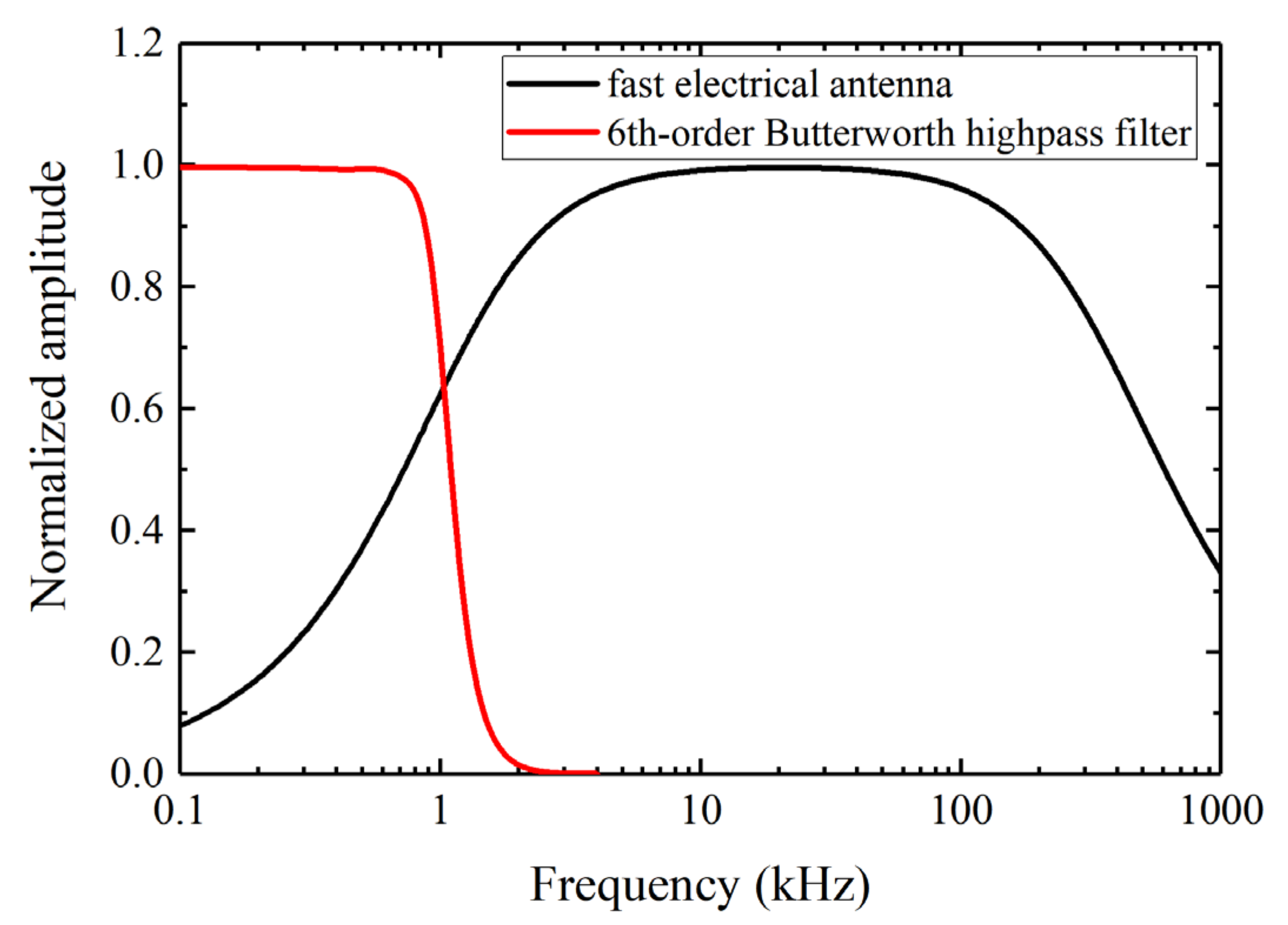
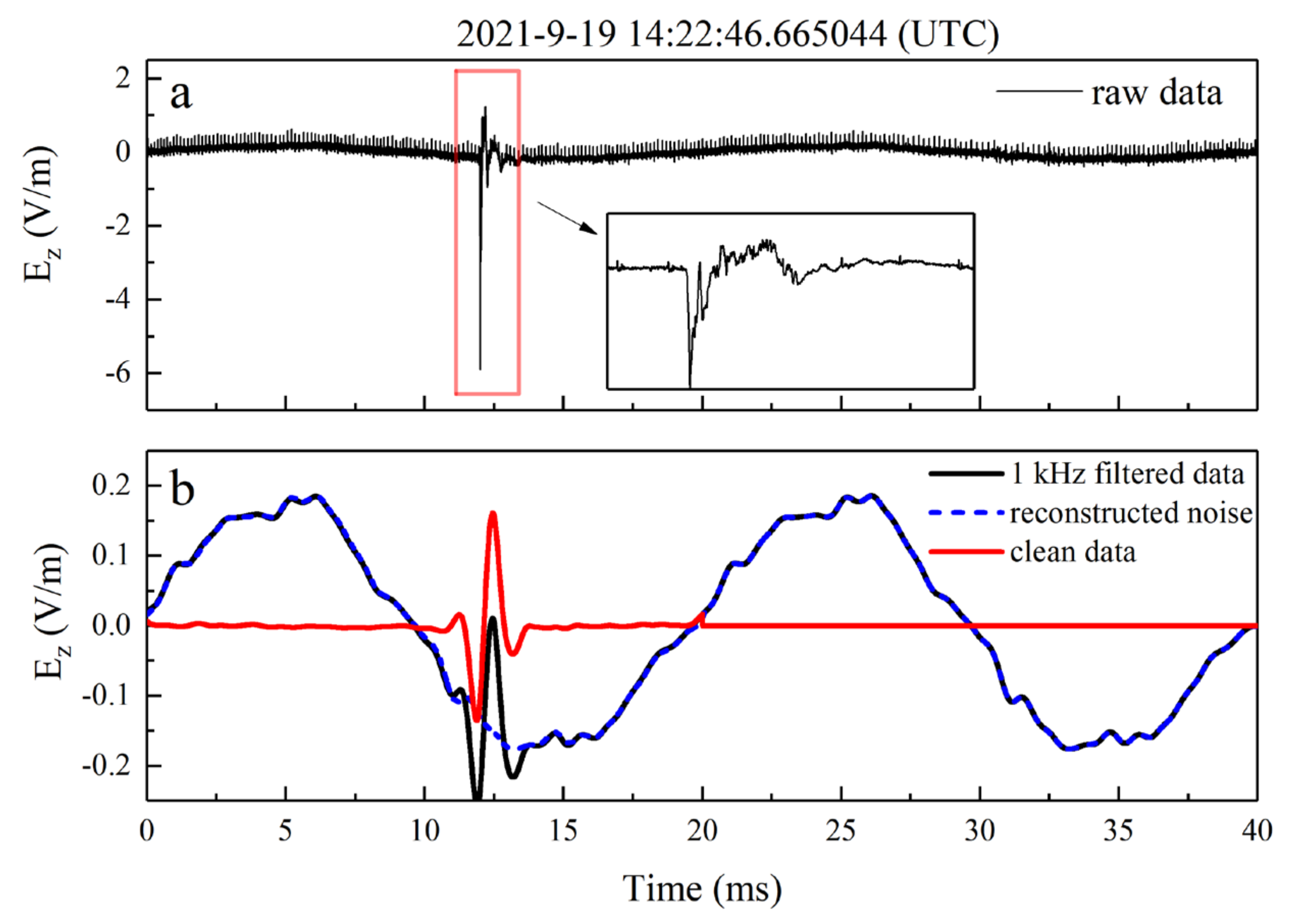
2.1. Instrument and Data

The fast electric field antenna (flat plate antenna) installed at the Nanjing University of Information Science and Technology (NUIST) (32.2065°N, 118.7170°E) was used. The 3-dB bandwidth of the fast antenna was 1.25 kHz to 350 kHz and its frequency response is shown in Figure 1 (black line). The site calibration factor was obtained by comparing the recorded electric field with that recorded on the ground level. A GPS receiver with an accuracy of ±50 ns was equipped at the station, and it provided a one-pulse-per-second output (1-PPS) as a reference source for data sample time tagging. The signals were sampled at 1 MHz.

In this study, only the signal below 1 kHz was used in the iCMC measurement. This is because there are pure QTEM waves in this band and the influence of the ionospheric parameters on the wave propagation is relatively less. On the contrary, in the VLF/LF band, due to the complicated waveguide propagation effects, the observed waveform is largely influenced by the ionospheric parameters [20,21,22]. A 6th-order Butterworth high-pass filter with cutoff of 1 kHz was applied to the recorded electric field. The red line in Figure 1 shows the frequency response of the high-pass filter. After filtering, the power line noise was reconstructed according to the data segment that does not contain lightning waveforms. Then, a clean electric field waveform could be obtained by subtracting the noise from the raw data.

Figure 2 shows an example of the data processing. Figure 2a shows a raw data measured by the fast antenna for a CG stroke. In Figure 2b, the black solid line is the waveform after the 1 kHz low-pass filtering. The blue dash line is the reconstructed noise waveform according to the adjacent waveform segment without lightning signal (20–40 ms), and it has a duration of 20 ms. The red line is the clean waveform obtained by subtracting the noise from the filtered waveform. It can be seen that the ELF waveform after the noise cancelation has a high signal-to-noise ratio.

The Jiangsu Advanced Direction and Time-of-Arrival Detecting (ADTD)-2 lightning data were used to identify the lightning location of the recorded lightning waveform. The Jiangsu ADTD-2 lightning locating network works in the VLF/LF band and includes 16 stations. It has a position accuracy less than ~500 m and time accuracy better than 2 μs in theory [23]. A match was found if the time difference between the calculated ADTD-lightning EM wave arrival time and the recorded wave arrival time by our antenna was less than 5 μs. When a match was found, the lightning location and propagation distance of the recorded lightning waveform were obtained. Then we simulated the impulse response at the distance.

2.2. Simulation of the Impulse Response

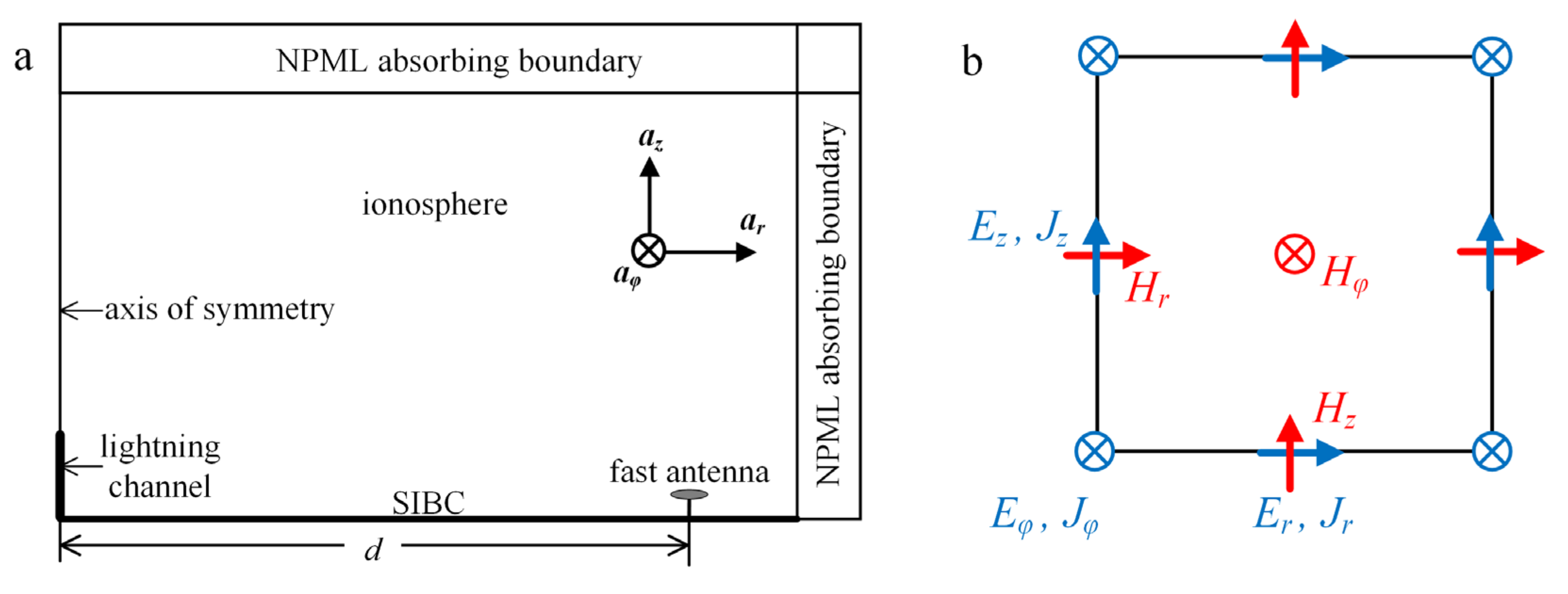
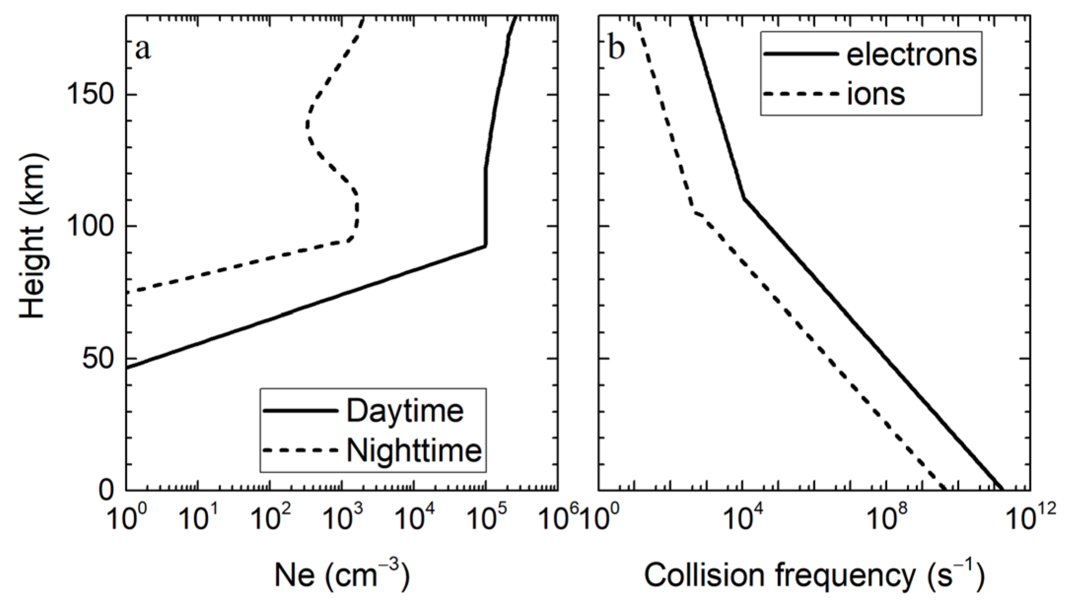
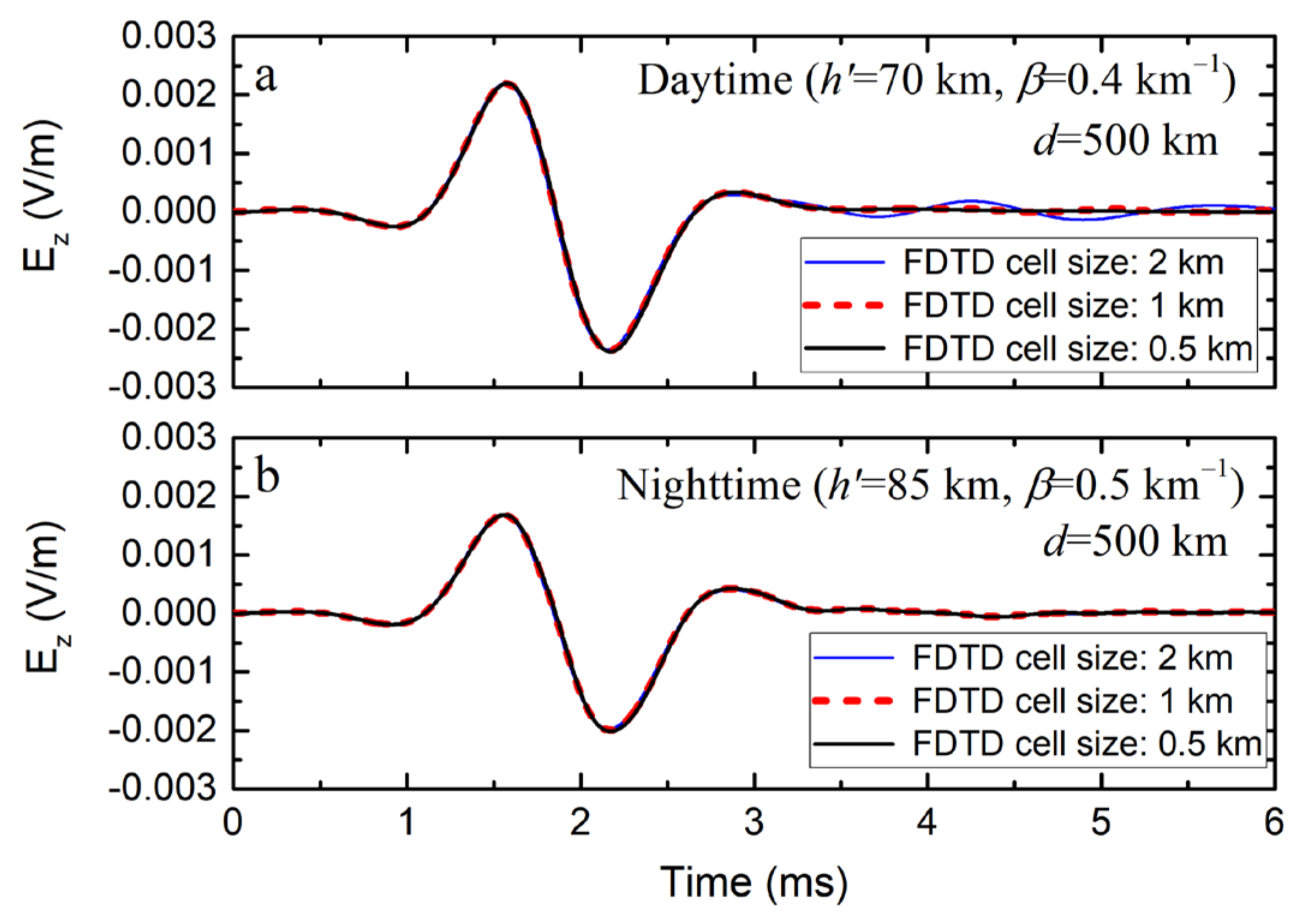
The impulse response of the EIWG is key to measure the lightning charge moment change. In this study, the impulse response was calculated using the finite difference time domain (FDTD) method. We will give a brief introduction of the FDTD and present an analysis on the impulse response in the time domain.

2.2.1. FDTD Model

The two-dimensional cylindrical FDTD code developed by Hou et al. [20] was used to simulate the propagation of the lightning electromagnetic pulse (LEMP) in the EIWG. This FDTD model was first developed by Hu and Cummer [24]. In this model, the lower ionosphere is regarded as a cold magnetized plasma, which is full of electrons, negative ions and positive ions. These charged particles move under the electric field, collide with neutral air and rotate under the geomagnetic field, generating the current in the ionosphere.

Figure 3a shows the overall FDTD configuration. The upper and right boundaries are surrounded by nearly perfectly matched layer (NPML)-absorbing boundaries [25]. The surface impedance boundary condition (SIBC) is applied to the bottom boundary to include the propagation effect. The Earth’s curvature is considered by modifying the refractive index at different heights [24]. The lightning channel is placed on the axis of symmetry. Figure 3b shows the mesh scheme of the FDTD model. The components of the electric field (E) and the current density (J) are collocated in time and space. The magnetic field (H) is shifted by half of the grid compared to E and J. The stability condition for the magnetized plasma is independent of medium properties and remains the same as that in free space when adopting the E–J method. More details of this FDTD model can be found in [24].

In the D region (<95 km) of ionosphere, a two-parameter exponential formulation is adopted to represent the electron density profile [26,27]

$$N_e\left(h\right)=1.43\times {10}^{13}{e}^{-0.15h^{\prime }}{e}^{\left(\beta -0.15\right)\left(h-h^{\prime }\right)}\left(m^{-3}\right)$$

(1)

where h is the height above the ground in km, h′ is the reference height of the ionosphere in km and β is the electron density profile sharpness in km⁻¹. h′ is set to 70 km and β is set to 0.4 km⁻¹ for a typical daytime ionosphere condition; h′ is set to 85 km and β is set to 0.5 km⁻¹ for a typical nighttime ionosphere condition [28,29]. The electron density in E region (about 95–170 km) is calculated using the International Reference Ionosphere—IRI 2016 [30] for a midlatitude region. Figure 4 shows the typical electron density profile under nighttime and daytime conditions and the collision frequencies of the electrons and ions [26].

By default, the Earth’s geomagnetic field was set to 50,000 nT and the geomagnetic inclination was set to 45° in the FDTD method. The angle between the horizontal component of ${\overrightarrow{B}}_E$ and the wave propagation direction was 0° (northward propagation). The lightning channel height was set to be 10 km. The FDTD simulation domain size was 500 km × 170 km, and the grid size was Δr = Δz = 1 km. The time step was Δt = 2 μs, which satisfies the Courant stability condition.

The FDTD code used in this study was validated in LF/VLF bands by Hou et al. [20] by comparing the simulated field waveform with the observed waveform. In Appendix A, we further validated our FDTD codes in the ELF bands using the transverse horizontal magnetic field recorded by Lu et al. [11] at Duke Forest Station (35.971°N, −79.094°E). A brief convergence study for the numerical grid is also presented and the results show that the cell size of 1 km was fine enough for our simulation.

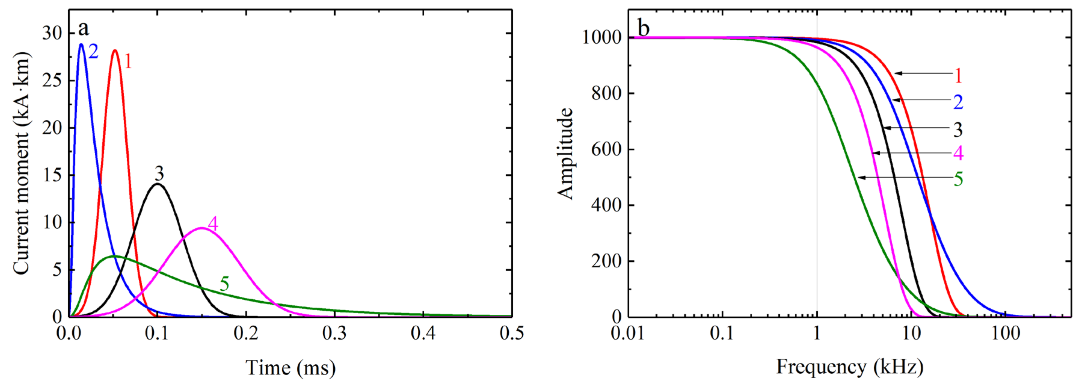
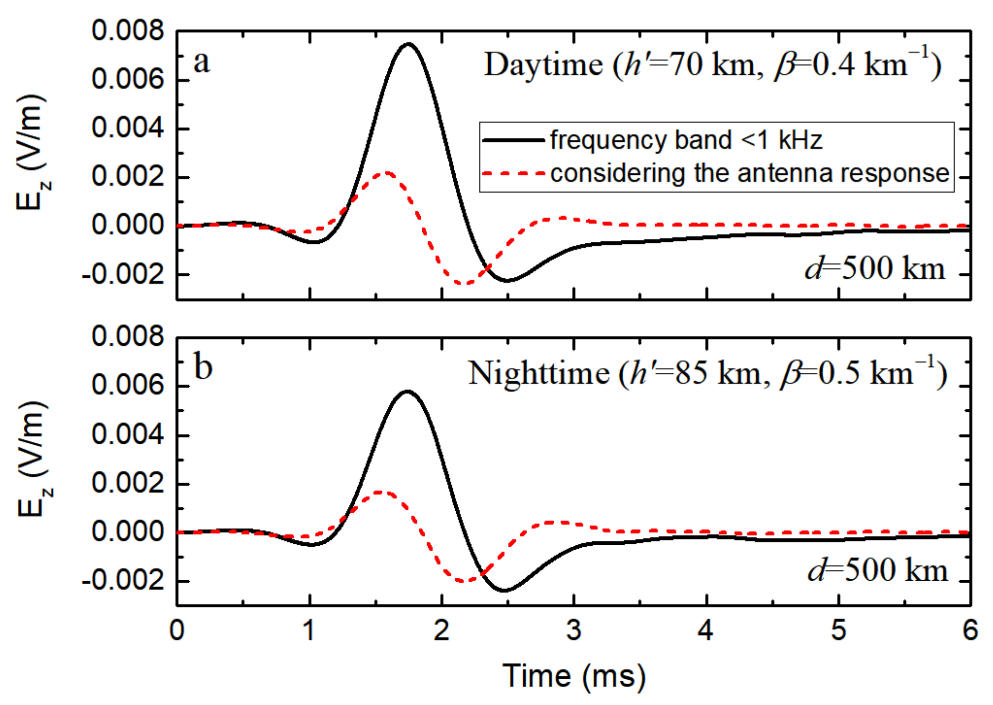
2.2.2. Modeled Impulse Response

In order to get the impulse response of the EIWG, an impulsive source needs to be inputted. Since the upper frequency limit of our concern was 1 kHz, the duration of the current moment needed to be much less than 1 ms. An impulsive current moment waveform in Gaussian shape with duration of 0.1 ms and charge moment change of 1 C·km was used in this study (see the red line in Figure 5a).

Here we will give some illustration on the use of the Gaussian-shaped current moment. Figure 5a shows several current moment waveforms which have different half-peak widths and different peaks. Their amplitude in the frequency domain is shown in Figure 5b. The time integrals of these current moments are all 1 C·km. The current moment waveforms numbered 1, 3 and 4 are all in Gaussian shape, with duration of 0.1 ms, 0.2 ms and 0.25 ms, respectively. The current moment waveforms numbered 2 and 5 have a fast rise time than fall time, and their durations are about 0.15 ms and 0.4 ms, respectively. It can be seen that the amplitude below 1 kHz is approximately a constant for the current moment numbered 1 to 4, no matter the differences in the current moment waveforms. In this situation, their radiated ELF field within 1 kHz will approximately be the same. Therefore, it is reasonable to use a Gaussian-shaped current moment to calculate the impulse response of the EIWG. In addition, the field waveform (or the field peak) radiated by an impulsive lightning discharge is determined by the time integral of the current moment which is the charge moment change, rather than the current moment waveform. It also can be seen that a discharge with duration less than ~0.25 ms can be regarded as an impulsive discharge in this study.

Figure 6 shows the modeled impulse responses within 1 kHz under typical daytime and nighttime conditions at the distance of 500 km. The black lines are the complete waveforms below 1 kHz, the red dash lines are the waveforms further considering our antenna response. It can be seen that the frequency response of the antenna has a significant influence on the impulse response. The bipolar characteristics of the waveforms are more obvious, and the field peak is largely reduced when the antenna response is applied. The impulse response considering the antenna response will be used in the measurement of iCMC.

The lower ionosphere is an anisotropic medium due to the presence of the geomagnetic field. In the VLF/LF band, the electron density profile in D region and the EM wave propagation direction have a large influence on the sky wave and its arrival time [20,21,22]. In Appendix B, the influence of the electron density profile in D region and the EM waveform propagation direction on the modeled impulse response in ELF band were studied. Results show that this influence is relatively less within 500 km. Therefore, the typical electron density profile is used, and a northward propagation of the EM wave is assumed in the following iCMC measurement.

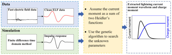
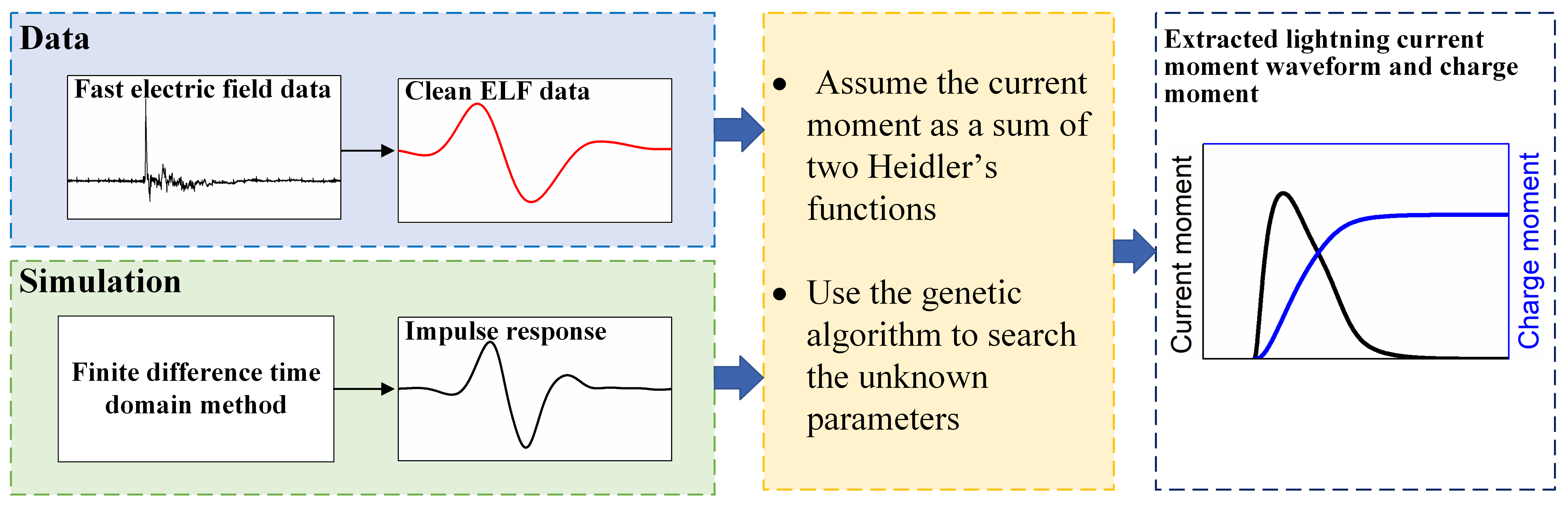
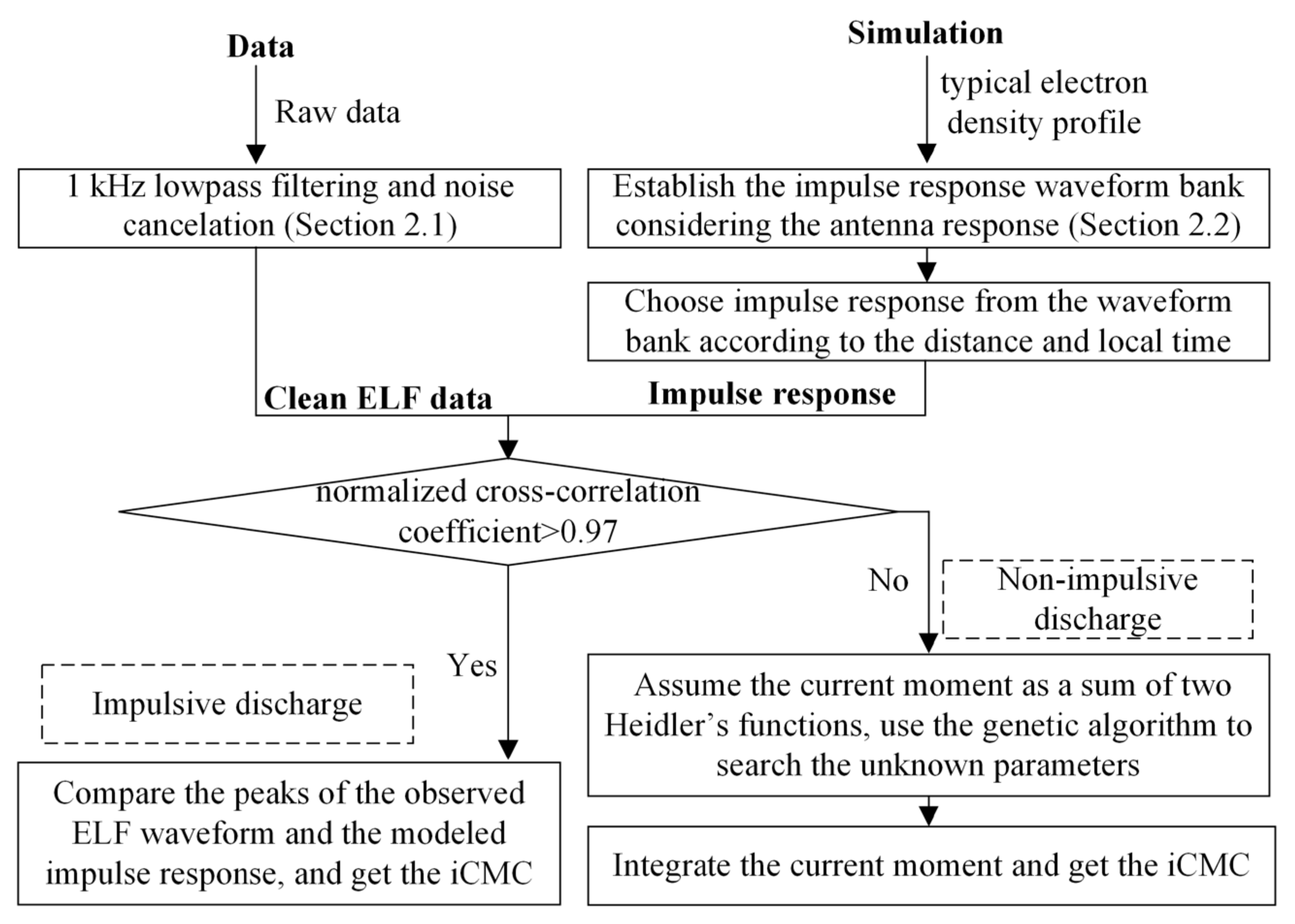
2.3. iCMC Measurement Method

With the observed ELF waveform described in Section 2.1 and the modeled impulse response in Section 2.2, we can measure the lightning iCMC.

Figure 7 shows the procedure of the iCMC measurement. Considering the typical electron density profiles in the daytime, nighttime and morning/evening condition, we can establish the modeled impulse response waveform bank using the FDTD method or other analytical method. For a recorded ELF waveform, choose the impulse response from the waveform bank according to the EM wave propagation distance and the local time. By comparing the observed waveform with the modeled impulse responses, we can infer whether the lightning discharge is an impulsive discharge. In this study, if the normalized cross-correlation coefficient between the observed ELF waveform and the modeled impulse response was larger than 0.97, the recorded ELF waveform was thought to be produced by an impulsive discharge; otherwise, this recorded ELF waveform was produced by the non-impulsive discharge. For the impulsive discharge, the observed ELF waveform and the modeled impulse response were highly similar. Since the field waveform and the field peak generated by an impulsive lightning discharge was determined by the charge moment, the iCMC could be obtained directly by the waveform comparison. For the non-impulsive discharge, the current moment waveform will be assumed to be the sum of two Heidler’s functions, and the genetic algorithm (GA) was used to search the unknown parameters in the function. In the following, we will focus on the non-impulsive lightning discharge and describe the method in detail.

For non-impulsive discharges, since the current moment waveform has a relatively broader pulse width, the generated ELF waveform will also have a broader pulse width compared with that produced by the impulsive discharge. In this case, the cross-correlation coefficient between the observed waveform and the impulse response is lower. In theory, the lightning current moment can be obtained by the deconvolution of the ELF field and the impulse response. However, the direct deconvolution method cannot guarantee the non-negativity and the smoothness of the obtained current moment waveform. Cummer and Inan [1] applied the linear regularization along with the projections onto the convex sets method to solve the problem. This method has been successfully used to measure the current moment waveforms, not only in the first several milliseconds but also in the long continuing current stage [9]. In this study we were only interested in the current moment waveforms in the first several milliseconds. The current moment waveform is assumed to be a sum of two Heidler’s functions, and the genetic algorithm is used to search the unknown parameters in the function.

2.3.1. Reconstructing the Current Moment Waveform Using Genetic Algorithm

The current moment (CM) waveform in the first several milliseconds is assumed to be a sum of two Heidler’s functions along with a Gaussian function, as shown in Equation (2).

$$\begin{array}{c}M\left(t\right)=\frac{A_1}{{\eta }_1}\frac{{(t/t_1)}^2}{[\left(t/t_1{)}^2+1\right]}{e}^{-t/t_2}+\frac{A_2}{{\eta }_2}\frac{{(t/t_3)}^2}{[\left(t/t_3{)}^2+1\right]}{e}^{-t/t_4}+A_3\mathit{exp}\left[-{\left(\frac{t-t_5}{t_6}\right)}^2\right]\hfill \\ {\eta }_1=\mathit{exp}\left[-\frac{t_1}{t_2}{\left(\frac{2t_2}{t_1}\right)}^{1/2}\right],\hspace{0.33em}{\eta }_2=\mathit{exp}\left[-\frac{t_3}{t_4}{\left(\frac{2t_4}{t_3}\right)}^{1/2}\right]\hfill \end{array}$$

(2)

where A₁, A₂ and A₃ control the amplitudes of the Heidler’s and Gaussian functions; t₁, t₂, t₃, t₄ and t₆ control the rise times and fall times of the waveforms; t₅ adjusts the position of the Gaussian function. The Gaussian function in the right hand of the equation is just an adjustment term used to adjust the rate of change of the current moment; it does not have much physical meaning.

First, we will give an explanation on the rationality of adopting the Heidler’s functions. In previous studies on the propagation of ELF electromagnetic pulses, which are also called the “slow tail” atmospherics, the lightning source is usually represented by the sum of exponential functions. Jones [31] summarized the lightning current parameters in previous literatures and derived a current moment formular used for the ELF propagation study, in which the leading current, the return stroke current and the continuing current are all expressed as exponential terms. In addition, according to the extracted current moment waveforms shown in Li [32], we can also see that the exponential function or the Heidler’s function is the proper choice to represent the lightning current moment waveforms in the first several milliseconds. Most importantly, since the upper frequency limit is 1 kHz in this study, the extracted current moment waveform can be regarded as a filtered result of the original real current moment. The extracted current moment will be one of the possible current moments, ignoring the fine structures in higher frequency. Since the sum of simple exponential functions cannot guarantee the current equals zero in the initial time, the Heidler’s function is adopted in the study. Therefore, Equation (2) is a reasonable representation to the lightning current moment waveform.

In Equation (2), there are nine unknown parameters (A₁-A₃, t₁-t₆). The current moment measurement problem is converted to finding suitable values for these unknown parameters to make the calculated ELF waveform fit the measured waveform. A fit parameter evaluating the error between the calculated ELF waveform (E_c) and the measured waveform (E_m) is defined as

$$\rho =\frac{1}{L}{\displaystyle \sum }_{n=1}^L\sqrt{{[E_m\left(t_n\right)-E_c\left(t_n\right)]}^2}$$

(3)

where t_n is the time and L is the number of samples in the waveforms. The calculated ELF waveform (E_c) is the convolution of the current moment (CM) and the impulse response. For different combinations of the parameter (A₁-A₃, t₁-t₆) values, we can get different CMs using Equation (2). By convoluting the CMs and the known impulse response, different simulated ELF waveforms can be obtained. Then, the parameter value set which minimizes the ρ in Equation (3) will be used to calculate the final current moment waveform.

In this study, the genetic algorithm [33] was used to determine the parameter values in the current moment waveform to give the best fit to the measured ELF waveform. The GA is a general optimization algorithm based on a random search technique, and the parameter search process mimics biological evolution. In previous studies, the genetic algorithm has been used to estimate the parameters in the lightning current functions (e.g., [34,35,36]). More introductions of GA can be found in these literatures.

Table 1. The lower limits and the upper limits of the parameters in Equation (2) used in this study.

Parameters	A1 (kA· km)	t1 (ms)	t2 (ms)	A2 (kA· km)	t3 (ms)	t4 (ms)	A3 (kA· km)	t5 (ms)	t6 (ms)
Lower limit	0	0.2	0	0	0.2	0	0	0	0.2
Upper limit	500	0.5	1	500	3	3	100	5	5

gives the allowed maximum and minimum values in GA for each parameter used in our measurement. The first Heidler’s function is designed to have a relatively narrow pulse width compared to the second one. The Gaussian function is set to have less amplitude than the Heidler’s function. These strategies contribute to the fast convergence of GA. The initial population is chosen to be 200, and the max generation (or iteration number) is set to 15.

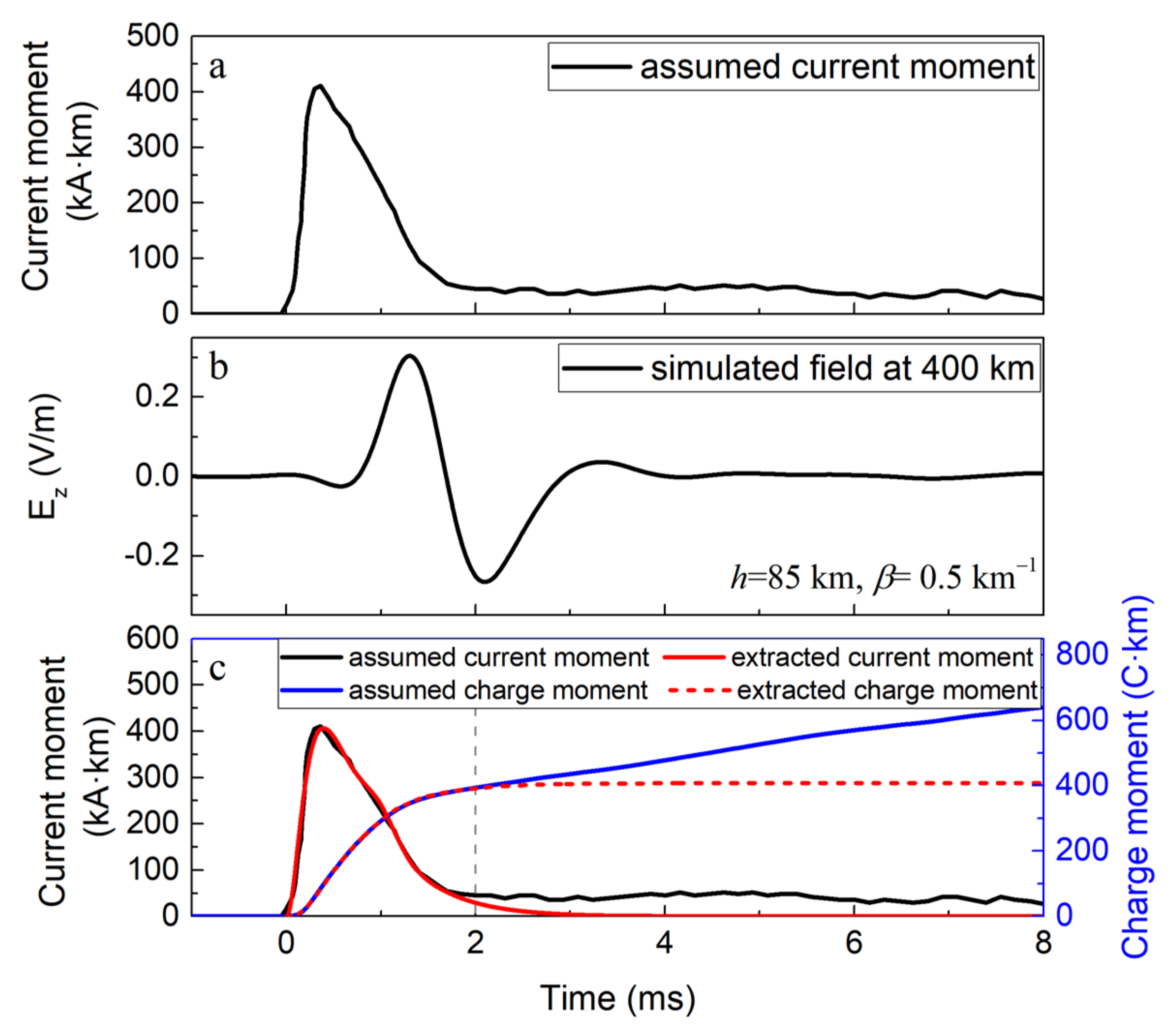
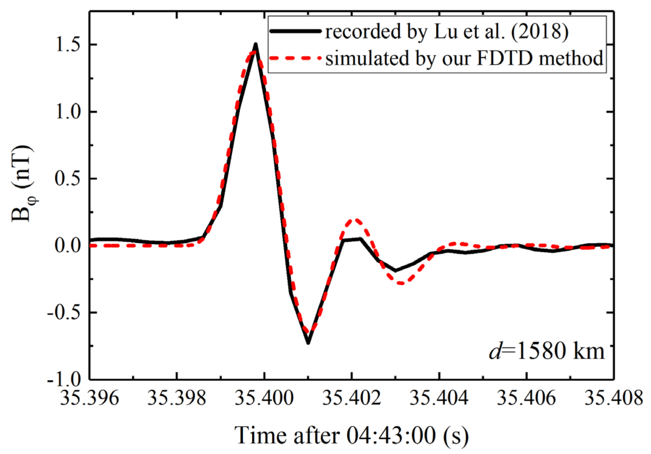
2.3.2. Method Validation

In this section, we test the proposed technique in order to check whether it can extract a reasonable current moment waveform and get the iCMC within 2 ms.

Figure 8a shows an assumed current moment waveform. This current moment waveform is adapted from [32]. It is composed of a long impulse current (0–2 ms) and a continuing current. Figure 8b shows the modeled vertical electric field waveform radiated by this current at distance of 400 km with ionospheric parameters h′ = 85 km and β = 0.5 km⁻¹. The frequency response of our fast antenna was considered. The modeled waveform is then used to extract the current moment waveform adopting the genetic algorithm. Figure 8c compares the extracted current moment waveform and charge moment waveform with the assumed ones. It can be seen that the extracted current moment waveform is almost the same with the assumed in the impulse current part. The extracted impulse charge moment within 2 ms is 392 C·km, and the assumed one is 394 C·km. This result validates that the proposed method using genetic algorithm is effective in the reconstruction of the current moment waveform, and it can really ensure the smoothness and non-negativity of the measured current moment waveform. In addition, it validates that the measured iCMC within 2 ms has a relatively high accuracy after considering the frequency response of the antenna, even the antenna gain falls with decreasing frequency.

3. Results

In the following section, we will present several examples to show how to get the iCMC for the impulsive discharge and the non-impulsive discharge, respectively.

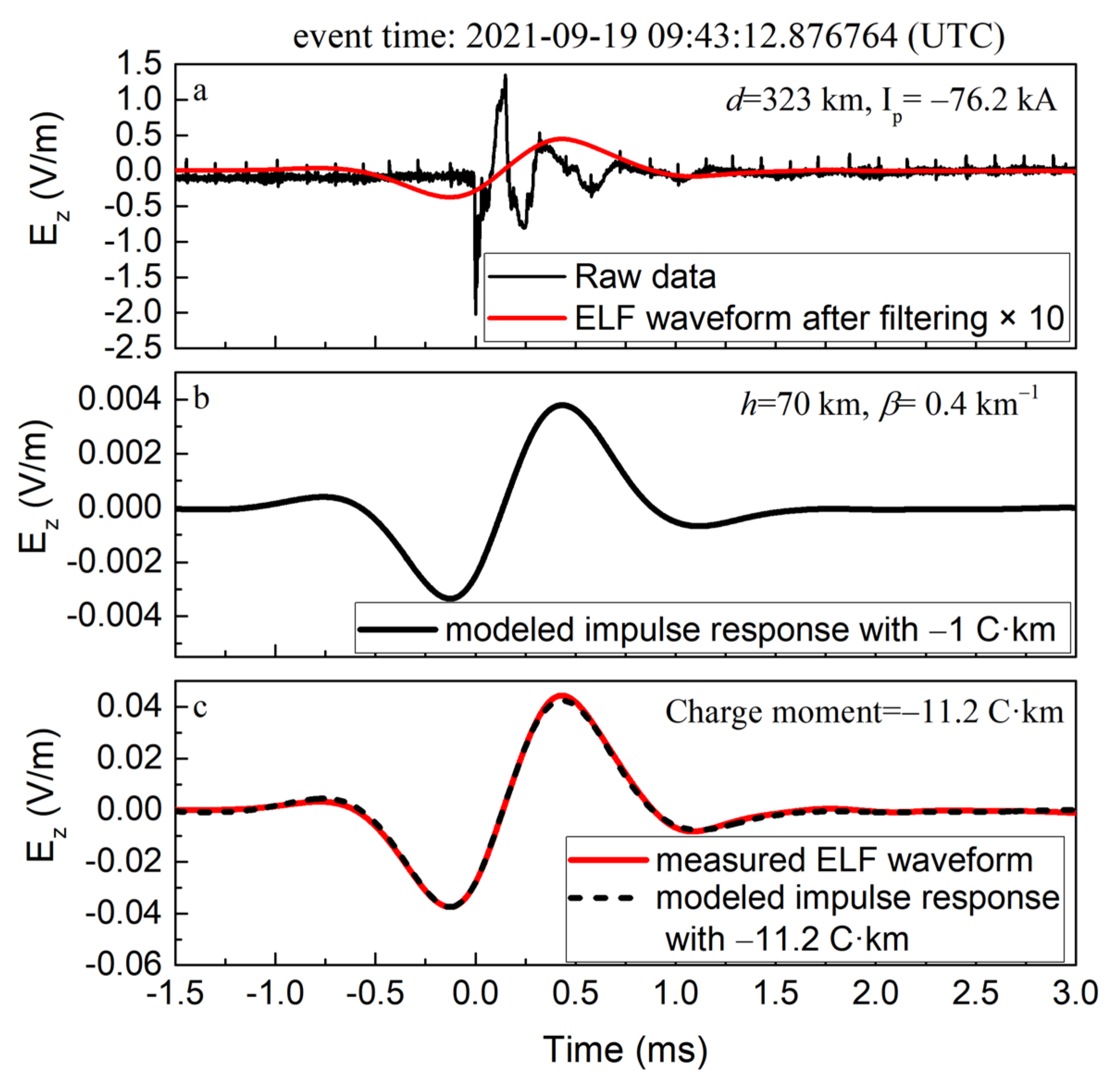
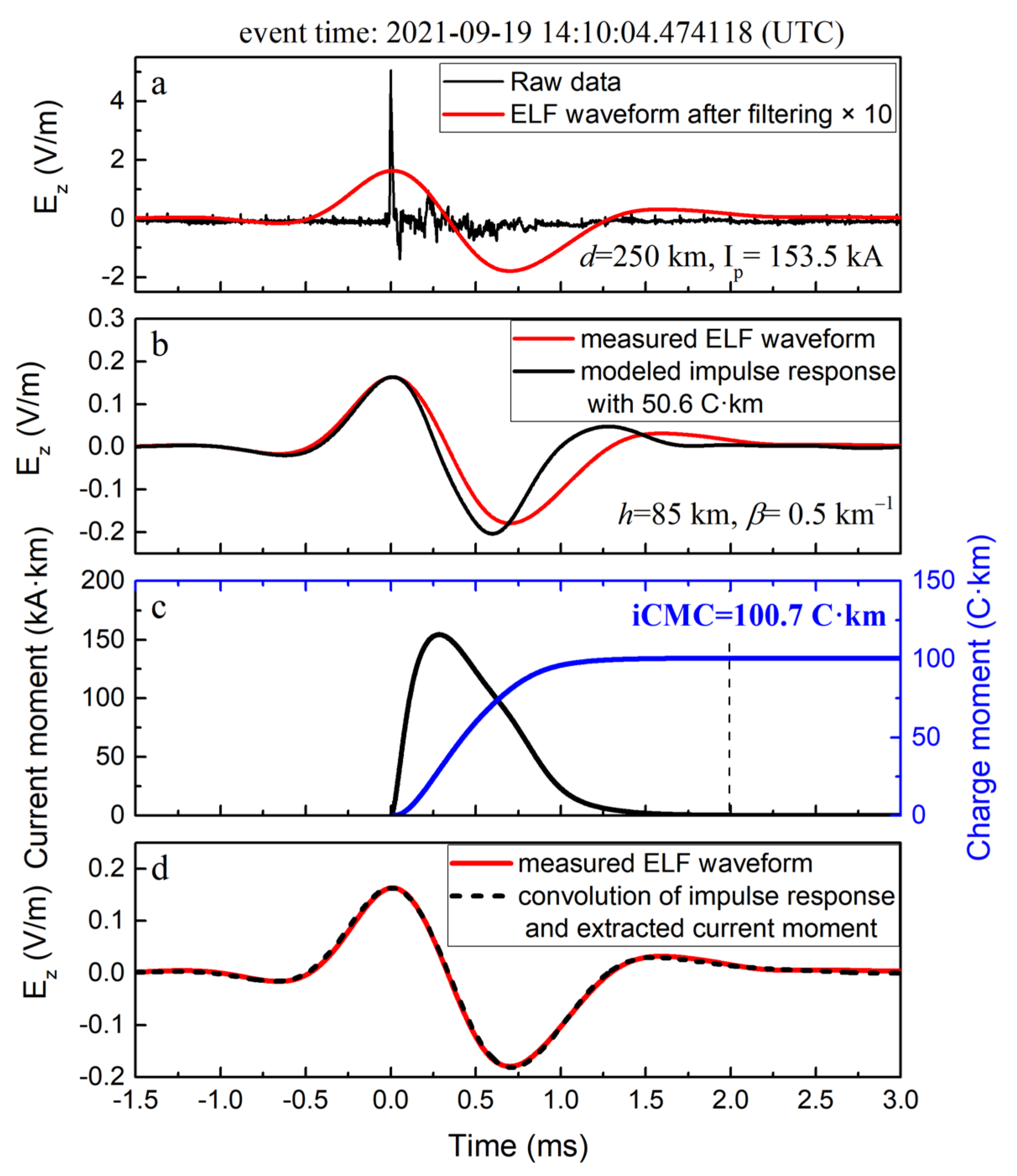
3.1. iCMC Measurement for the Impulsive Discharge

Figure 9a shows the vertical electric field recorded by the NUIST station at 09:43:12.877840 UT on 19 September 2021. It was produced by a negative flash with peak current of −76.2 kA at distance of 323 km, according to the ADTD-2 lightning locating data. The black line is the raw data and the red line is the ELF waveform after the noise cancelation. It was found that the cross-correlation coefficient between the observed waveform and the modeled impulse response at the distance of 323 km with h’ = 70 km and β = 0.4 km⁻¹ is 0.998. We can infer that this ELF waveform is produced by an impulsive discharge whose duration is less than 0.25 ms.

As shown in Figure 9c, after enlarging the simulated impulse response by 11.2 times, the simulated waveform is approximately identical to the observed one. Therefore, the charge moment of this negative lightning discharge is about −11.2 C·km. More calculation results show that the iCMC ranges from −11.2 to −12.9 C·km when h’ ranges from 70 to 74 km and β ranges from 0.3 to 0.4 km⁻¹.

Figure 10 shows another example similar to Figure 9 but under a nighttime condition. The return stroke peak current is −89.9 kA, and the distance is 213 km away from the NUIST station. The measured ELF waveform (red line in Figure 10c) and the modeled impulse response with −24.8 C·km (black dash line in Figure 10c) have an excellent agreement, indicating the charge moment of this lightning discharge is about −24.8 C·km. The measured iCMC ranges from −23.2 to −24.9 C·km when h’ ranges from 82 to 87 km and β ranges from 0.5 to 0.7 km⁻¹. The maximum value of the relative error is about 6.6% when ignoring the influence of the electron density profile. This indicates that our method is not sensitive to the ionospheric parameters.

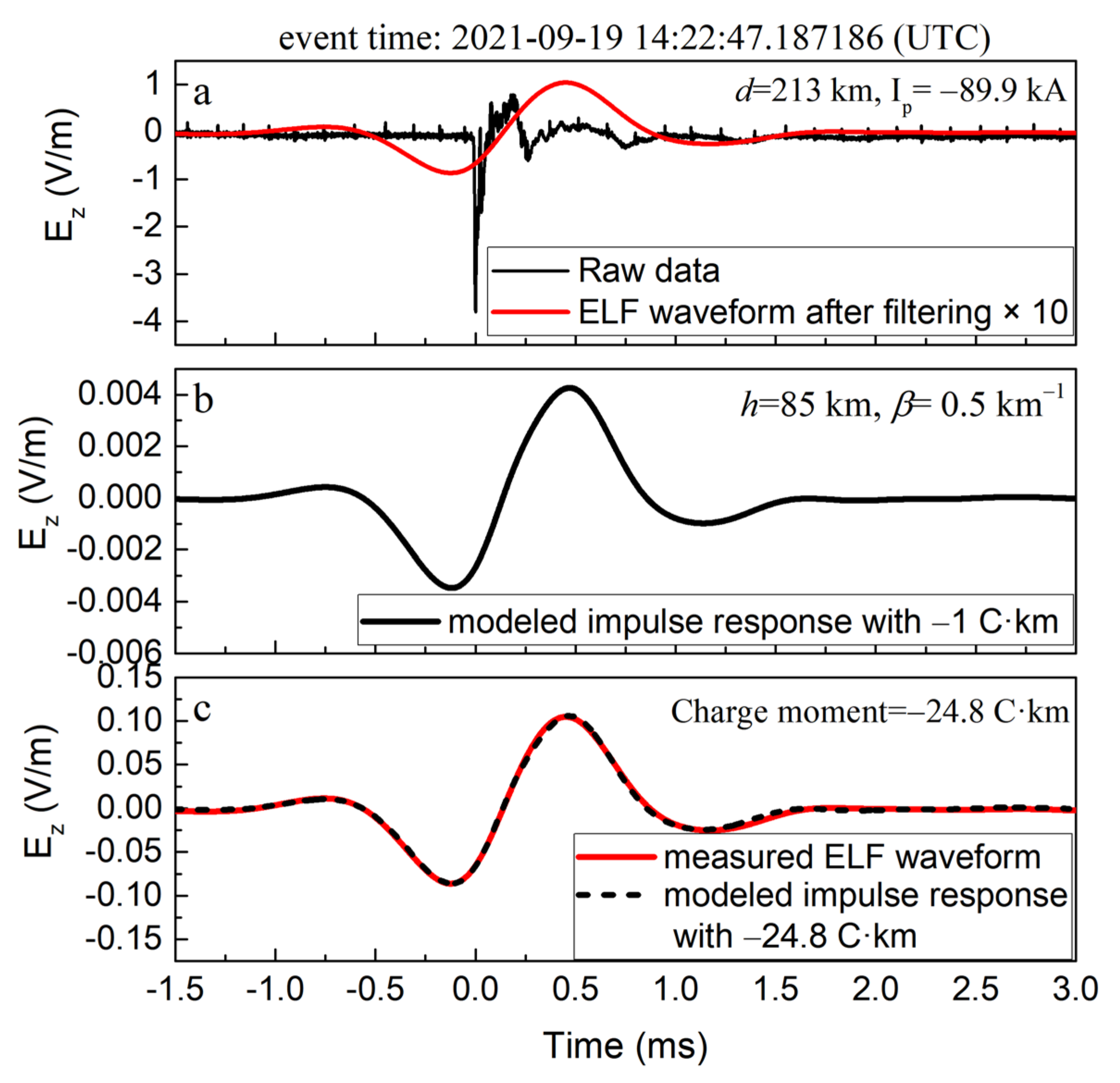
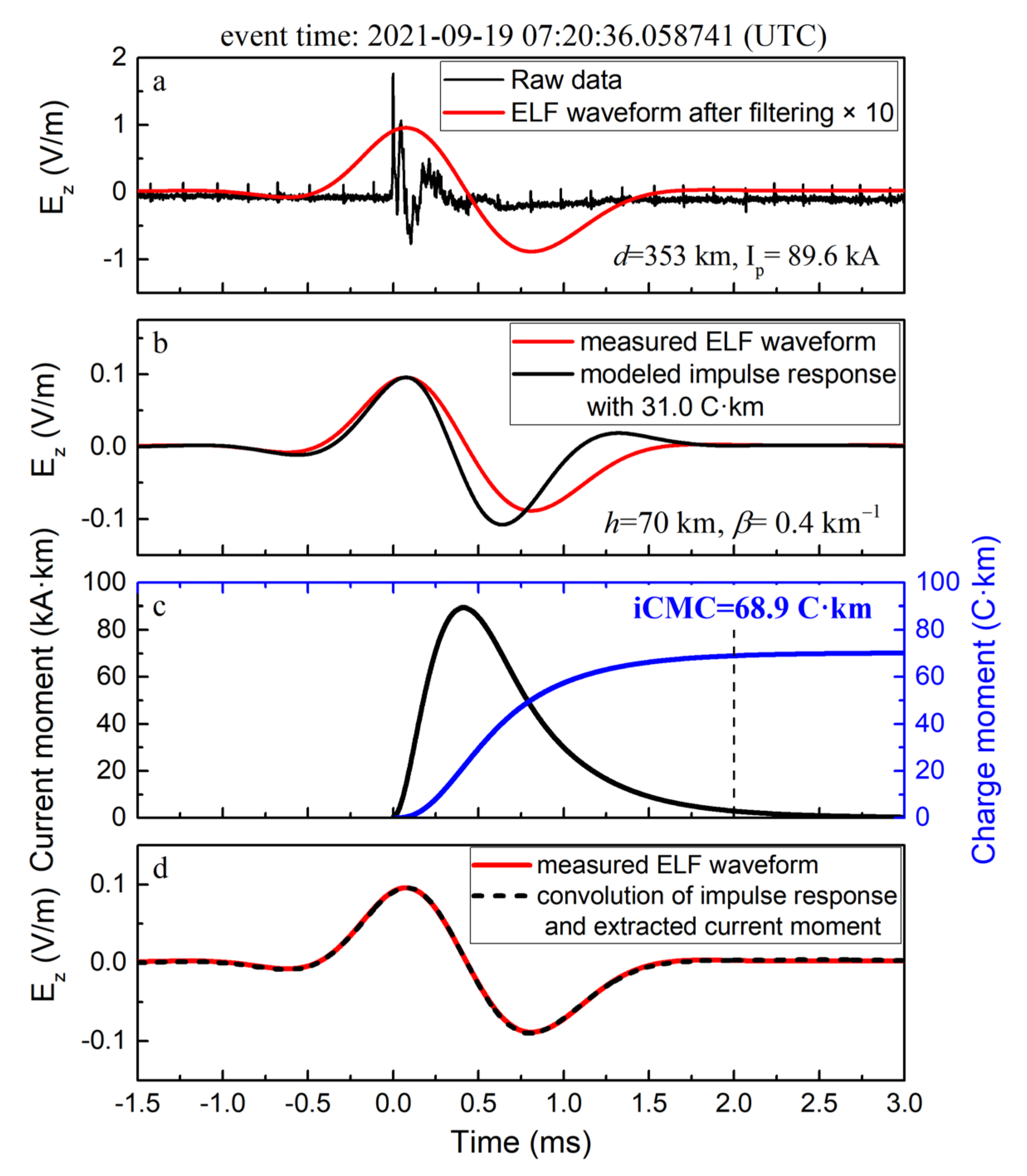
3.2. iCMC Measurement for the Non-Impulsive Discharge

Figure 11 shows an example of iCMC measurement for a non-impulsive CG lightning discharge in the nighttime. It was produced by a positive flash with peak current of 153.5 kA at distance of 250 km. The raw data (black line) and the ELF waveform after the noise cancelation (red line) are shown in Figure 11a. The cross-correlation coefficients between the observed ELF waveform and the modeled impulse response at distance of 250 km are lower than the threshold, indicating the field is radiated by a non-impulsive discharge. Figure 11b shows the comparison of the measured ELF waveform and the modeled impulse response with 50.6 C·km. Although their field peak is the same, the measured waveform has a larger width and zero-crossing time, implying the charge moment is larger than 50.6 C·km. Then, its current moment waveform is assumed to be a sum of two Heidler’s functions, and the genetic algorithm is used to search the unknown parameters. Figure 11c shows the extracted current moment waveform using GA and the charge moment waveform. The duration of the reconstructed current moment is ~1.5 ms, which is larger than the duration of the impulsive discharge (being ~0.25 ms in this study). The measured iCMC within 2 ms is 100.7 C·km. Figure 11d compared the measured ELF waveform with the waveform obtained by the convolution of the impulse response and the extracted current moment waveform. The good agreement implies that the extracted current moment waveform is reasonable.

Table 2. Measured iCMC and relative errors considering different ionospheric parameters and geomagnetic field parameters for the example shown in Figure 11.

No.	Ionospheric Parameters	Geomagnetic Field Parameters *	EM Wave Propagation Direction	iCMC (C·km)	Relative Errors	Remark
1	h’ = 82 km, β = 0.5 km−1	I = 45°	0°	97.9	2.2%
2	h’ = 85 km, β = 0.5 km−1	I = 45°	0°	100.6	5.0%	shown in Figure 11
3	h’ = 87 km, β = 0.5 km−1	I = 45°	0°	105.9	10.5%
4	h’ = 82 km, β = 0.7 km−1	I = 45°	0°	102.5	7.0%
5	h’ = 85 km, β = 0.7 km−1	I = 45°	0°	105.3	9.9%
6	h’ = 87 km, β = 0.7 km−1	I = 45°	0°	111.1	16.0%
7	h’ = 85 km, β = 0.5 km−1	I = 50°, D = −6°	150°	95.8	—	set as reference

* I is the geomagnetic inclination, D is the geomagnetic declination.

summarizes the calculated iCMC and the relative errors under different ionospheric parameters. The result considering the real EM wave propagation direction and the average geomagnetic field parameters between the lightning strike point and the observation station is also presented and was set as reference. I is the geomagnetic inclination. D is the geomagnetic declination, and a negative value means the geomagnetic field is rotated west from true north. It can be seen that the maximum value of the relative error is about 16% when β increases from 0.5 km⁻¹ to 0.7 km⁻¹. Compared with the result only considering the EM wave propagation direction, the calculated iCMC increased by only 5%. These results are consistent with the analysis presented in Appendix B, implying that the influence of the wave propagation on the iCMC measurement within several hundred kilometers can be approximately ignored.

Figure 12 shows another example of iCMC measurement for a non-impulsive CG lightning discharge in the daytime. It was produced by a positive flash with peak current of 89.6 kA at a distance of 353 km. The difference between the measured ELF waveform and the modeled impulse response shown in Figure 12b indicates this is a non-impulsive lightning discharge. The duration of the extracted current moment (see Figure 12c) using GA is ~2.5 ms, which is much larger than 0.25 ms. The measured iCMC is 68.9 C·km. The measured ELF waveform and the waveform calculated by the convolution of the impulse response and the extracted current moment waveform have a good agreement.

Table 3. Measured iCMC and relative errors considering different ionospheric parameters and geomagnetic field parameters for the example shown in Figure 12.

No.	Ionospheric Parameters	Geomagnetic Field Parameters *	EM Wave Propagation Direction	iCMC (C·km)	Relative Errors	Remark
1	h’ = 70 km, β = 0.3 km−1	I = 45°	0°	61.1	−11.4%
2	h’ = 74 km, β = 0.3 km−1	I = 45°	0°	69.7	1.0%
3	h’ = 70 km, β = 0.4 km−1	I = 45°	0°	68.9	−0.1%	shown in Figure 12
4	h’ = 74 km, β = 0.4 km−1	I = 45°	0°	73.5	6.5%
5	h’ = 70 km, β = 0.4 km−1	I = 51°, D = −6°	165°	69.0	—	set as reference

* I is the geomagnetic inclination, D is the geomagnetic declination.

further shows the error analysis considering different ionospheric parameters and geomagnetic field parameters. The maximum relative error is −11.4%, and the error without considering the real geomagnetic field parameters and the EM wave propagation direction is only −0.1%, implying our method is robust.

4. Discussion

In Section 3, the influence of the anisotropic ionosphere on the iCMC measurement was analyzed in detail. Results show that this influence can be approximately ignored within ~500 km. In practical terms, the electron density profile in D region in real time can be obtained by the methods developed in the VLF/LF band (e.g., [21,28,29,37]). The measured electron density profile parameters can be used to calculate the impulse response and then used for a more accurate iCMC measurement.

It is worth noting that the extracted current moment waveform is a low-pass filtered version of the original real current moment since the upper frequency limit is 1 kHz in our method. However, this does not limit the measurability of the charge moment change which is the time integral of the current moment, because the time integrals of a function f(t) and a low-pass filtered function f_filt(t) are the same [2].

Single-station data were used in this study. The method can be easily extended to the multi-station measurement by revising the fit parameter in Equation (3), as in the work by Karunarathne et al. [38], in which 10 electric field sensors were used to measure the currents of initial breakdown pulses. For the multi-station measurement, we can define the normalized fit parameter as

$$\rho =\frac{1}{N}{\displaystyle \sum }_{i=1}^N{\displaystyle \sum }_{n=1}^{L_i}\sqrt{\frac{1}{L_n}{\left[\frac{E_{mi}\left(t_n\right)-E_{ci}\left(t_n\right)}{\Delta E_{mi,pp}}\right]}^2}$$

(4)

where N is the station number, L_i is the number of samples in the waveform of the ith sensor. E_ci is the calculated ELF waveform at ith station, E_mi is the measured waveform at ith station. $\Delta E_{mi,pp}$ is the measured peak to peak electric field of ith sensor.

The frequency bandwidth of our fast antenna is mainly in LF/VLF band. The reason why we can measure the current moment and iCMC in the ELF band is that the frequency response of the antenna is compensated for in the modeled impulse response. However, the frequency response dramatically falls with decreasing frequency. The gain in the lower frequency is too small to distinguish the corresponding waveform component in the complete waveform. Therefore, compared with the previous studies conducted using the ELF magnetic antenna, the method presented in this paper cannot be used to extract the current moment in the continuing current. However, considering the wide use and the relatively easy development of the fast antenna, this technique can be easily extended and used for the continuous monitoring of the lightning iCMC in a given time and space.

5. Conclusions

In this paper, we developed a new method to measure the lightning iCMC within 2 ms at distances of several hundreds of kilometers. The method is based on the vertical electric field measured by the widely used fast antenna with LF/VLF band. The impulse response of EIWG is modeled using a FDTD method. By comparing the observed waveform with the simulated impulse response, the lightning discharge is classified into the impulsive discharge and the non-impulsive discharge. For the impulsive discharge, its iCMC is obtained directly by comparing the measured ELF waveform to the modeled impulse response. For the non-impulsive discharge, its current moment waveform is assumed to be a sum of two Heidler’s functions, and the genetic algorithm is used to search the unknown parameters in the function. The good agreement between the measured ELF waveform and the simulated waveform implies that the extracted current moment is consistent with the data.

References

1. Cummer, S.A.; Inan, U. Modeling ELF radio atmospheric propagation and extracting lightning currents from ELF observations. Radio Sci. 2000, 35, 385–394. [Google Scholar] [CrossRef] [Green Version]
2. Cummer, S.A. Current moment in sprite-producing lightning. J. Atmos. Sol.-Terr. Phys. 2003, 65, 499–508. [Google Scholar] [CrossRef]
3. Cummer, S.A.; Lyons, W.A.; Stanley, M.A. Three years of lightning impulse charge moment change measurements in the United States. J. Geophys. Res. Atmos. 2013, 118, 5176–5189. [Google Scholar] [CrossRef]
4. Lu, G.; Cummer, S.A.; Blakeslee, R.J.; Weiss, S.; Beasley, W.H. Lightning morphology and impulse charge moment change of high peak current negative strokes. J. Geophys. Res. Space Phys. 2012, 117, D04212. [Google Scholar] [CrossRef] [Green Version]
5. Lyu, F.; Cummer, S.A.; McTague, L. Insights into high peak current in-cloud lightning events during thunderstorms. Geophys. Res. Lett. 2015, 42, 6836–6843. [Google Scholar] [CrossRef]
6. Cummer, S.A.; Inan, U.S. Measurement of charge transfer in sprite-producing lightning using ELF radio atmospherics. Geophys. Res. Lett. 1997, 24, 1731–1734. [Google Scholar] [CrossRef] [Green Version]
7. Huang, E.; Williams, E.; Boldi, R.; Heckman, S.; Lyons, W.; Taylor, M.; Nelson, T.; Wong, C. Criteria for sprites and elves based on Schumann resonance observations. J. Geophys. Res. Earth Surf. 1999, 104, 16943–16964. [Google Scholar] [CrossRef]
8. Hu, W.; Nelson, T.E.; Cummer, S.A.; Lyons, W.A. Lightning charge moment changes for the initiation of sprites. Geophys. Res. Lett. 2002, 29, 1279. [Google Scholar] [CrossRef] [Green Version]
9. Li, J.; Cummer, S.A.; Lyons, W.A.; Nelson, T.E. Coordinated analysis of delayed sprites with high-speed images and remote electromagnetic fields. J. Geophys. Res. Earth Surf. 2008, 113, D20206. [Google Scholar] [CrossRef] [Green Version]
10. Kułak, A.; Młynarczyk, J. A new technique for reconstruction of the current moment waveform related to a gigantic jet from the magnetic field component recorded by an ELF station. Radio Sci. 2011, 46, RS2016. [Google Scholar] [CrossRef] [Green Version]
11. Lu, G.; Yu, B.; Cummer, S.A.; Peng, K.; Chen, A.B.; Lyu, F.; Xue, X.; Liu, F.; Hsu, R.; Su, H. On the Causative Strokes of Halos Observed by ISUAL in the Vicinity of North America. Geophys. Res. Lett. 2018, 45, 10781–10789. [Google Scholar] [CrossRef]
12. Kulak, A.; Mlynarczyk, J.; Ostrowski, M.; Kubisz, J.; Michalec, A. Analysis of ELF electromagnetic field pulses recorded by the Hylaty station coinciding with terrestrial gamma-ray flashes. J. Geophys. Res. Earth Surf. 2012, 117, D18203. [Google Scholar] [CrossRef] [Green Version]
13. Lu, G.; Zhang, H.; Cummer, S.A.; Wang, Y.; Lyu, F.; Briggs, M.; Xiong, S.; Chen, A. A comparative study on the lightning sferics associated with terrestrial gamma-ray flashes observed in Americas and Asia. J. Atmos. Sol.-Terr. Phys. 2019, 183, 67–75. [Google Scholar] [CrossRef]
14. Jones, D.; Kemp, D. The nature and average magnitude of the sources of transient excitation of Schumann resonances. J. Atmos. Terr. Phys. 1971, 33, 557–566. [Google Scholar] [CrossRef]
15. Wood, T.G.; Inan, U.S. Long-range tracking of thunderstorms using sferic measurements. J. Geophys. Res. Earth Surf. 2002, 107, ACL 1-1–ACL 1-9. [Google Scholar] [CrossRef]
16. Krehbiel, P.R.; Brook, M.; McCrory, R.A. An analysis of the charge structure of lightning discharges to ground. J. Geophys. Res. Earth Surf. 1979, 84, 2432–2456. [Google Scholar] [CrossRef]
17. Qie, X.; Yu, Y.; Liu, X.; Guo, C.; Wang, D.; Watanabe, T.; Ushio, T. Charge analysis on lightning discharges to the ground in Chinese inland plateau (close to Tibet). Ann. Geophys. 2000, 18, 1340–1348. [Google Scholar] [CrossRef]
18. Nieckarz, Z.; Baranski, P.; Mlynarczyk, J.; Kulak, A.; Wiszniowski, J. Comparison of the charge moment change calculated from electrostatic analysis and from ELF radio observations. J. Geophys. Res. Atmos. 2015, 120, 63–72. [Google Scholar] [CrossRef]
19. Heidler, F.; Cvetic, J.; Stanic, B. Calculation of lightning current parameters. IEEE Trans. Power Deliv. 1999, 14, 399–404. [Google Scholar] [CrossRef]
20. Hou, W.; Azadifar, M.; Rubinstein, M.; Rachidi, F.; Zhang, Q. The Polarity Reversal of Lightning-Generated Sky Wave. J. Geophys. Res. Atmos. 2020, 125, e2020JD032448. [Google Scholar] [CrossRef]
21. Qin, Z.; Chen, M.; Zhu, B.; Du, Y.-P. An improved ray theory and transfer matrix method-based model for lightning electromagnetic pulses propagating in Earth-ionosphere waveguide and its applications. J. Geophys. Res. Atmos. 2017, 122, 712–727. [Google Scholar] [CrossRef]
22. Tran, T.H.; Baba, Y.; Somu, V.; Rakov, V.A. FDTD Modeling of LEMP Propagation in the Earth-Ionosphere Waveguide With Emphasis on Realistic Representation of Lightning Source. J. Geophys. Res. Atmos. 2017, 122, 12918–12937. [Google Scholar] [CrossRef]
23. Zhou, X.; Wang, J.; Ma, Q.; Huang, Q.; Xiao, F. A method for determining D region ionosphere reflection height from lightning skywaves. J. Atmos. Sol.-Terr. Phys. 2021, 221, 105692. [Google Scholar] [CrossRef]
24. Hu, W.; Cummer, S. An FDTD Model for Low and High Altitude Lightning-Generated EM Fields. IEEE Trans. Antennas Propag. 2006, 54, 1513–1522. [Google Scholar] [CrossRef]
25. Cummer, S.A. A simple, nearly perfectly matched layer for general electromagnetic media. IEEE Microw. Wirel. Compon. Lett. 2003, 13, 128–130. [Google Scholar] [CrossRef] [Green Version]
26. Wait, J.R.; Spies, K.P. Characteristics of the Earth-Ionosphere Waveguide for VLF Radio Waves (NBS Tech. Note 300); National Bureau of Standards: Boulder, CO, USA, 1964. Available online: https://nvlpubs.nist.gov/nistpubs/Legacy/TN/nbstechnicalnote300.pdf (accessed on 2 February 2022).
27. Thomson, N. Experimental daytime VLF ionospheric parameters. J. Atmos. Terr. Phys. 1993, 55, 173–184. [Google Scholar] [CrossRef]
28. Han, F.; Cummer, S.A. Midlatitude daytime D region ionosphere variations measured from radio atmospherics. J. Geophys. Res. Earth Surf. 2010, 115, A10314. [Google Scholar] [CrossRef] [Green Version]
29. Han, F.; Cummer, S.A. Midlatitude nighttime D region ionosphere variability on hourly to monthly time scales. J. Geophys. Res. Earth Surf. 2010, 115, A09323. [Google Scholar] [CrossRef]
30. Bilitza, D.; Altadill, D.; Truhlik, V.; Shubin, V.; Galkin, I.; Reinisch, B.; Huang, X. International Reference Ionosphere 2016: From ionospheric climate to real-time weather predictions. Space Weather 2017, 15, 418–429. [Google Scholar] [CrossRef]
31. Jones, D. Electromagnetic radiation from multiple return strokes of lightning. J. Atmos. Terr. Phys. 1970, 32, 1077–1093. [Google Scholar] [CrossRef]
32. Li, J. Coordinated Analysis of Sprites with High Speed Images and Remote Electromagnetic Fields. Ph.D. Thesis, Duke University, Durham, UK, 2010. [Google Scholar]
33. Goldberg, D.E. Genetic Algorithms in Search, Optimization and Machine Learning; Addison-Wesley Longman Publishing Co., Inc.: Reading, MA, USA, 1989. [Google Scholar]
34. Bermudez, J.L.; Pena-Reyes, C.A.; Rachidi, F.; Heidler, F. Use of genetic algorithms to extract primary lightning current parameters. In Proceedings of the EMC Europe 2002 International Symposium on Electromagnetic Compatibility, Sorrento, Italy, 9–13 September 2002; pp. 241–246. [Google Scholar]
35. Chandrasekaran, K.; Punekar, G.S. Use of Genetic Algorithm to Determine Lightning Channel-Base Current-Function Parameters. IEEE Trans. Electromagn. Compat. 2014, 56, 235–238. [Google Scholar] [CrossRef]
36. Javor, V.; Lundengård, K.; Rančić, M.; Silvestrov, S. Application of Genetic Algorithm to Estimation of Function Parameters in Lightning Currents Approximations. Int. J. Antennas Propag. 2017, 2017, 4937943. [Google Scholar] [CrossRef] [Green Version]
37. Shao, X.-M.; Lay, E.; Jacobson, A.R. Reduction of electron density in the night-time lower ionosphere in response to a thunderstorm. Nat. Geosci. 2013, 6, 29–33. [Google Scholar] [CrossRef]
38. Karunarathne, S.; Marshall, T.C.; Stolzenburg, M.; Karunarathna, N. Modeling initial breakdown pulses of CG lightning flashes. J. Geophys. Res. Atmos. 2014, 119, 9003–9019. [Google Scholar] [CrossRef]
Figure 1. The normalized frequency response of our fast electric field antenna (black line) and the 6th-order Butterworth high-pass filter with cutoff of 1 kHz (red line).
Remotesensing 14 00724 g001
Figure 2. An example of the data processing. (a) Raw data, (b) noise cancelation process.
Remotesensing 14 00724 g002
Figure 3. (a) FDTD configuration. (b) Mesh scheme of the FDTD model. The positions of the vector components in ar, az and aφ directions are shown.
Remotesensing 14 00724 g003
Figure 4. (a) Typical electron density profile under nighttime and daytime conditions. The density of positive ions is set to the same value as the electrons but with a minimum value of 200 cm−3 in daytime and 100 cm−3 in nighttime. (b) Collision frequencies of the electrons and the positive and negative ions.
Remotesensing 14 00724 g004
Figure 5. (a) Five current moment waveforms with different rise and fall times. Their time integrals are all 1 C·km. The red line labeled 1 represents the impulsive current moment source used to calculate the impulse response in this study. (b) The corresponding amplitude in frequency domain.
Remotesensing 14 00724 g005
Figure 6. Modeled impulse response for 1 C·km at 500 km in the typical (a) daytime and (b) nighttime condition. The black lines are the complete waveforms below 1 kHz, the red dash lines are the waveforms further considering our antenna response. Note that ahead of the waveform, initial time compared with d/c (c being the light speed) is caused by the zero-phase filter.
Remotesensing 14 00724 g006
Figure 7. Procedure of the iCMC measurement.
Remotesensing 14 00724 g007
Figure 8. (a) Assumed current moment waveform. (b) Calculated ELF field below 1 kHz at distance of 400 km considering our fast antenna. This field waveform is in turn used to calculate the current moment waveform. (c) Comparison of the assumed current waveform and the calculated waveform using GA.
Remotesensing 14 00724 g008
Figure 9. Demonstration of a charge moment measurement from ELF vertical electric field for an impulsive CG lightning discharge with peak current of −76.2 kA at distance of 323 km in daytime. The event time in the title is the return stroke time. (a) The raw data (black line) and the ELF waveform after the noise cancelation (red line). (b) Modeled impulse response with h’ = 70 km and β = 0.4 km−1 at distance of 323 km. (c) Comparison of the measured ELF waveform (red line) and the modeled impulse response (black dash line) with −11.2 C·km.
Remotesensing 14 00724 g009
Figure 10. Similar to Figure 9, but for an impulsive CG lightning discharge at a distance of 213 km in nighttime. The measured ELF waveform (red line in Figure 10c) and the modeled impulse response with −24.8 C·km (black dash line in Figure 10c) have an excellent agreement, indicating the iCMC is about −24.8 C·km.
Remotesensing 14 00724 g010
Figure 11. ICMC measurement for a non-impulsive CG lightning discharge at 14:10:04.474118 UT on 19 September 2021. (a) The raw data (black line) and the ELF waveform after the noise cancelation (red line). (b) Modeled impulse response with h’ = 85 km and β = 0.5 km−1 at distance (d) of 250 km. The difference in waveforms indicates the field is radiated by a non-impulsive discharge. (c) The extracted current moment waveform and charge moment waveform using the proposed method. (d) Comparison of the measured ELF waveform (red line) and the modeled waveform (black dash line). The measured and the modeled field waveforms are nearly identical.
Remotesensing 14 00724 g011
Figure 12. Similar to Figure 11. ICMC measurement for a non-impulsive CG lightning discharge at 07:20:36.058741 UT on 19 September 2021. This is an example in daytime. The calculated iCMC is 68.9 C·km.
Remotesensing 14 00724 g012