
Hybrid Variability Aware Network (HVANet): A Self-Supervised Deep Framework for Label-Free SAR Image Change Detection


National Laboratory of Radar Signal Processing, Xidian University, Xi’an 710071, China
*
Author to whom correspondence should be addressed.
Remote Sens. 2022, 14(3), 734; https://0-doi-org.brum.beds.ac.uk/10.3390/rs14030734
Submission received: 30 December 2021
/
Revised: 26 January 2022
/
Accepted: 31 January 2022
/
Published: 4 February 2022
(This article belongs to the Special Issue Image Change Detection Research in Remote Sensing)
Abstract
:Synthetic aperture radar (SAR) image change detection (CD) aims to automatically recognize changes over the same geographic region by comparing prechange and postchange SAR images. However, the detection performance is usually subject to several restrictions and problems, including the absence of labeled SAR samples, inherent multiplicative speckle noise, and class imbalance. More importantly, for bitemporal SAR images, changed regions tend to present highly variable sizes, irregular shapes, and different textures, typically referred to as hybrid variabilities, further bringing great difficulties to CD. In this paper, we argue that these internal hybrid variabilities can also be used for learning stronger feature representation, and we propose a hybrid variability aware network (HVANet) for completely unsupervised label-free SAR image CD by taking inspiration from recent developments in deep self-supervised learning. First, since different changed regions may exhibit hybrid variabilities, it is necessary to enrich distinguishable information within the input features. To this end, in shallow feature extraction, we generalize the traditional spatial patch (SP) feature to allow for each pixel in bitemporal images to be represented at diverse scales and resolutions, called extended SP (ESP). Second, with the carefully customized ESP features, HVANet performs local spatial structure information extraction and multiscale–multiresolution (MS-MR) information encoding simultaneously through a local spatial stream and a scale-resolution stream, respectively. Intrinsically, HVANet projects the ESP features into a new high-level feature space, where the change identification becomes easier. Third, to train the framework effectively, a self-supervision layer is attached to the top of the HVANet to enable the two-stream feature learning and recognition of changed pixels in the corresponding feature space, in a self-supervised manner. Experimental results on three low/medium-resolution SAR datasets demonstrate the effectiveness and superiority of the proposed framework in unsupervised SAR CD tasks.
1. Introduction
Benefiting from the capability of all-weather and all-time Earth observation, the synthetic aperture radar (SAR) sensor has been used in numerous applications increasingly, including but not limited to urban planning, disaster monitoring, and land-cover/land-use (LCLU) analysis [1,2,3,4,5,6,7]. In reality, change detection (CD) in SAR images is crucial in these applications, which seeks to precisely identify the changed and unchanged parts by analyzing two or more SAR images acquired over the same geographic region at different times [2,3,7,8,9]. However, SAR images exhibit diversified inherent characteristics, such as ubiquitous multiplicative speckle noise and geometrical distortions, that inevitably impose some challenges in SAR image CD [8,9,10].
The challenges of SAR image CD mainly come from three aspects: (1) the speckle noise and pseudochange [3,9,10,11,12], (2) the scarcity of accessible labeled samples, and (3) class imbalance [13].
- 1.
- Speckle Noise and Pseudochange: Due to the particular imaging mechanism that creates SAR images by processing the radar backscatter responses coherently [10,11], speckle noise inevitably appears all over the images, which dramatically affects the intensity of the SAR images; consequently, changed pixels share a wide range of intensity values with unchanged pixels, namely intensity fluctuations. This is because speckle causes dramatic intensity fluctuations and further results in the overlapped nature between the changed and unchanged classes [9,10], which brings difficulty for accurate change feature extraction. In addition, pseudochanges can also be caused by the slight variation of the acquisition parameters, such as the imaging configuration, incidence angles, and radiometric variations, making it difficult to detect changes of interest precisely [14,15].
- 2.
- Scarcity of Labeled Samples: It is acknowledged that collecting a large quantity of high-quality pixel-wise annotations in a short time is infeasible, raising the problem of training data scarcity. On the one hand, the problem poses challenges for the existing supervised CD approaches [13] that rely heavily on either ground truth or a significant amount of labeled training samples. On the other hand, the absence of label information makes it difficult for the unsupervised methods [9,11,12,14,15,16,17,18,19] that rely on handcrafted features to model the change information accurately.
- 3.
- Class Imbalance: Considering that the prior probability of occurrence of changed objects is much lower than unchanged ones, SAR CD is a typical class imbalance classification issue in practical scenarios. That is to say, the number of changed pixels is much smaller than unchanged ones in the context of bitemporal SAR scenes. Such an imbalance problem will severely undermine the performance of data-driven approaches [13]. However, almost all existing methods overlook this problem.
In summary, all these problems together form the major obstacles for SAR CD and impede the detection performance from improving, which motivates us to explore a more effective model further. By reviewing the existing literature, the above issues are usually addressed from the perspectives of difference image (DI) generation (i.e., shallow feature extraction), classifier design, and sample selection strategy.
Firstly, to capture discriminant change features and counteract the speckle effect, researchers have developed a series of DI generation methods, including but not limited to mathematical difference descriptors [20,21,22,23] and statistical modeling [24,25,26,27], such as the log-ratio operator [21], wavelet-based DI fusion methods [23,28,29], likelihood-ratio method [27], and multiresolution analysis-based method [28], etc. Recently, saliency detection has been employed to robustly locate the conspicuous changed regions and to remove the easily confusable regions in the background, such that better quality can be gained in the produced DI [30,31,32]. However, these saliency-guided methods focus on long-range contextual information at the expense of details due to the inevitable blurring effect.
Secondly, most previous SAR image CD works [8,9,11,12,14,15,16,17,18,19] focus on how to design an unsupervised model to achieve good performance, wherein clustering-based classifiers [9,15,17,18,28] are considered most representative and popular. Although their effectiveness and efficiency have been demonstrated, traditional clustering algorithms still suffer from some significant drawbacks, the major one of which is the poor ability in data fitting. Recently, deep learning models, such as the autoencoder [30], convolutional neural network (CNN) [33], and capsule network [34], have been adopted to accurately process the complex and nonlinear SAR data, where pseudolabels inferred by clustering algorithms are used as supervised signals. These methods are regarded as a novel CD framework named the preclassification scheme. Even if this scheme alleviates the scarcity of labeled samples to a certain extent, the label information is still derived from the clustering, whose accuracy cannot be ensured. Consequently, this may lead to image CD systems that cannot learn exact change semantics. More recently, some studies [11,35] have resorted to transfer learning, thus providing an alternative solution to the problem of labeled data scarcity. Transfer learning can make use of prior knowledge in the source domain (e.g., optical data with/without ground truth) to train a deep network for application in the target domain (i.e., SAR data). However, the distribution discrepancy between the target and source domains cannot be easily bridged, restricting the performance of transfer learning-based methods.
As for the class imbalance in SAR data, very few methods have tried to explicitly provide a practical and feasible solution, such as [13], where the ground truth map is utilized to guide the training data set construction in a supervised manner. We argue that the strategy in [13] is inapplicable in practical SAR scenarios where accurate labels are costly and expensive to collect. Among the existing unsupervised methods [30,31,32,33,34,35,36,37,38,39,40], this problem has always been neglected, where training instances of changed and unchanged classes are usually sampled from the imbalanced class distributions, further leading to the imbalance in the training set. Considering that this problem will inevitably hinder the model training, a specialized strategy is necessary to rebalance the class distributions in the training data set to learn class knowledge better.
Apart from the aforementioned problems, changed regions in bitemporal SAR scenes tend to occur at various sizes in arbitrary orientations and also exhibit highly varied shapes and textures, typically summarized as “hybrid variabilities”. Specifically, changed regions usually occupy connected areas ranging from a dozen of pixels to thousands of pixels, the so-called scale variation. Furthermore, the changes that occur between bitemporal images may correspond to various natural or manmade objects, which are naturally exhibited as irregular shapes and somewhat different textures in images. All these hybrid variabilities together increase the difficulty of accurately recognizing real changed parts. Although a large number of SAR image CD methods have been proposed, none of them has put enough emphasis on this unique characteristic inherently existing in changed regions.
In this article, we propose a label-free SAR CD system to comprehensively tackle all these problems, which formulates the local structure information learning and the multiscale–multiresolution (MS-MR) information encoding into a unified framework to strengthen the feature distinguishability and fulfill the classification in a completely unsupervised way. It includes three parts: shallow feature extraction, the class rebalance strategy, and the training of the Hybrid Variability Aware Network (HVANet). At first, considering the importance of the context information in describing images, we generalize the conventional single-scale spatial patch (SP) feature to focus on the MS-MR information for the representation at each image pixel, referred to as extended SP (ESP). The key novelty of the feature extraction is MS-MR patch feature construction, which can greatly help to characterize both image details and semantic content from multiple levels and perspectives. Second, a class rebalance strategy is proposed to realize a manageable balance in the training data set. Third, for the purpose of the label-free detection of changes, a self-supervised network named HVANet is specially tailored for completely unsupervised feature learning and change identification. Specifically, we establish two streams in HVANet to concurrently learn local structure information and encode MS-MR information, referred to as the local spatial stream and the scale-resolution stream. Intrinsically, HVANet projects the input ESP features into a new learned feature space in a self-supervised manner, where pixels of different categories with diverse appearances can be better differentiated. Finally, training and inference can be performed end-to-end. The main contributions of this paper can be summarized as follows:
- 1.
- We define a completely unsupervised SAR image CD framework, under which a novel label-free method is accomplished. Specifically, the idea of self-supervised learning is introduced to enable end-to-end high-level feature learning and classifier training without any labeled samples.
- 2.
- We propose to represent each pixel in the images using both the conventional single-scale patch (i.e., SP feature) and the MS-MR patches simultaneously, which is capable of comprehensively describing pixel information through the complementary local spatial information and long-range context information. These features are gathered together as the shallow feature for each pixel, from which the network can extract multiple types of high-level features for better feature representation and feature classification.
- 3.
- We devise a novel two-stream network architecture called HVANet, which decomposes the feature learning into the local spatial and the scale-resolution streams. The local spatial stream employs the Siamese network (SiamNet) to extract the intrinsic structural information around each pixel, while the scale-resolution stream encodes the corresponding MS-MR information to compensate for the spatial context for intensifying representation power.
The rest of this paper is organized as follows. Section 2 reviews the existing unsupervised SAR image CD works. Section 3 presents in detail the proposed label-free CD framework for SAR images. Experimental results are presented in Section 4. Finally, the discussions and conclusions are provided in Section 5 and Section 6, respectively.
2. Related Work
SAR image CD is one of the challenging scene understanding tasks in the SAR community. In the literature, the process of CD typically consists of change feature extraction and feature classification. Accordingly, we review the existing CD methods from these two perspectives: change feature extraction and feature classification.
(1) Change Feature Extraction: Feature extraction in CD, known for its capability to generate DI or features focusing on change information, is a key step. At the very beginning, some mathematical operators, such as the subtraction, ratio, and log-ratio operators [20,21,22,23], are adopted to measure change information pixel-by-pixel, thus deriving a DI. Most of the operators are often susceptible to speckle and pseudochanges. Then, considering the better representation ability inherent in the spatial context, a variety of methods have been exploited to improve the accuracy and robustness of change information measurement by leveraging the wavelet-related algorithms [23,28,29,31,33,36] due to their ability to extract multiscale (or multiresolution) context information. However, it has been observed that wavelet transform cannot fully characterize the real changes in complex scenes. Recently, some strategies [30,31,32] have been dedicated to making use of the saliency information obtained by considering long-range dependencies in images and have thus been able to effectively reduce distraction in the complex background. Typically, Geng et al. [30] use a segmented saliency map as the binary spatial weight for the log-ratio DI to filter the distraction in the background. Unfortunately, these saliency-guided methods [30,31,32] suffer from a major drawback: they can enhance context but inevitably induce a blurring effect to edge and image details due to their emphasis on global information; thus, the changed regions may be shrunken or dilated, causing a great deal of misclassified pixels near the borders and finally detail loss.
(2) Feature Classification: This process aims to assign a label (changed or unchanged semantic label) for each pixel, following which the class labels are mosaiced to a change map. The process can be roughly categorized into two classes, i.e., supervised and unsupervised, based on whether labels are necessary or not. Considering the labeled data scarcity, unsupervised classifiers are preferable in feature classification where no ground-truth labels are required, thus relieving the reliance on real labels. The representative methods of this kind typically use the feature extraction techniques described above to acquire low-level handcrafted features and directly use clustering models to obtain a change map, as shown in Figure 1a. In this direction, Aiazzi et al. [15], Celik [17], Gong, Zhou, and Ma [27] have made many remarkable advances in unsupervised SAR CD. Although they have been shown to be effective, the conventional clustering models are susceptible to speckle and pseudochanges and fail to make a precise decision because of their weak fitting capability under complex SAR data distribution.
Stepping into the era of artificial intelligence, recent years have witnessed an increasing interest in deep learning methods to address a number of problems in remote sensing (RS) image analysis and interpretation. In this context, a deep learning-based preclassification scheme has been recently developed, as shown in Figure 1b, which casts the unsupervised problem into a supervised deep learning problem. Under the scheme, a shallow unsupervised classifier is first applied to assign pseudolabels to unlabeled samples, following which deep models can be effectively trained in a supervised way. Here, clustering models mainly serve as the shallow classifier [30,32,33,34,37,38,39,40], which means that methods under this scheme remain clustering-guided. In [36], Gong et al. firstly proposed a pioneering deep neural network (DNN)-based SAR image CD approach. Afterward, a variety of works [30,32,33,34,38,39,40] have followed this scheme to take advantage of the superiority of deep learning techniques in automatic feature learning and classification. Despite the good achievements achieved, the weak data fitting ability of the critical clustering-based shallow classifier causes two main limitations: i) the pattern diversity of the pseudolabeled training samples is overly simple, and ii) noisy labels are inevitable. As a consequence, both the diversity and credibility of the pseudolabeled samples cannot be ensured, hindering the training and finally limiting the generalization performance of deep models.
With the development of deep learning technology, there is a new trend of SAR image CD that exploits the newly proposed transfer learning paradigm to circumvent the limitations thanks to a domain knowledge transfer trait [11,35,41]. The rationale is to exploit a large amount of accessible heterogeneous images with/without ground truth to pretrain a deep model and then transfer it into the target data domain in the fine-tuning stage. In this regard, it helps to efficiently reduce the reliance of deep models on labeled samples in the target domain where pixel-wise annotations are very difficult and costly to gather. Gao et al. [35] use 10 multitemporal SAR images with ground truth to train a CD network, which is transferred to the considered SAR scene for CD through a fine-tuning operation. Tan et al. [41] introduce the idea of transfer learning into the dictionary learning for PolSAR CD. Saha et al. [11] build an SAR-optical transcoding network to implement SAR image CD in the feature space of the optical domain. Nevertheless, the data shift between two different data domains caused by the vast difference in imaging mechanisms is a gap that is not easy to bridge, thus limiting the domain knowledge transfer performance.
Recently, thanks to its ability to effectively mine category knowledge for model learning through the nature of unlabeled data, self-supervised learning, served as a special branch of unsupervised learning, has been prevailing in the context of RS image interpretation [42,43,44]. Specific for self-supervised learning, the learning signal can be constructed by uncovering and exploiting the latent structure and nature in unlabeled data, while the entire training procedure is completely label-free [45]. Notably, self-supervised learning figures out an effective fashion to fully exploit the unlabeled samples to excavate underlying category knowledge and learn useful features for some downstream tasks, such that the scarcity of labeled samples can be tackled to a certain extent. However, existing self-supervised learning-based CD works [46,47,48] almost focus on multispectral/hyperspectral images [46] or cross-sensor images [47,48]. In [47], Chen and Bruzzone explored building a self-supervised pseudo-Siamese network for multispectral-SAR images CD based on contrastive learning. It constructs positive samples using the bitemporal images from the same scene and constructs the negative samples using paired images from different scenes, such that the network is trained end-to-end in an unsupervised way. Finally, the cross-sensor bitemporal images can be compared by the deep features extracted by the pseudo-Siamese network. In [48], Saha et al. proposed a CD framework for optical-SAR image CD using a self-supervised model. To the best of our knowledge, few studies have investigated the self-supervised CD methods purely for bitemporal SAR images so far. As a consequence, the intrinsic challenges in SAR data still remain. It is necessary to explore a self-supervised framework to overcome the challenges in SAR image CD.
In this work, we exploit self-supervised learning to realize an end-to-end and label-free learning of the task-specific high-level features from original bitemporal SAR images. To this end, a self-supervised learning paradigm is used to enable label-free feature learning and change identification. As shown in Figure 1c, thanks to the label-free property of self-supervised learning, real labels are unnecessary in the training process, such that the preclassification scheme and its defects can be avoided and a completely unsupervised deep learning-based CD framework can be established.
3. The Proposed Method
Denote the bitemporal single-channel SAR images acquired over the same geographic region at two different times and as and of the same size , where H and W refer to height and width, respectively. In bitemporal SAR images, the geometry and appearances of different changed regions may be significantly different, typically manifested by the high variabilities in size, shape, and texture, which are not trivial to model. In addition, the other challenges, including the scarcity of labeled data, the speckle effect, and the class imbalance problem, also severely restrict the performance and generalization of the detection model.
Our goal is to overcome these challenges, that is, precisely locating the real changes between and while keeping the number of false and missed changes low. To this end, we propose a self-supervised framework to make full use of latent category knowledge in unlabeled samples for the purpose of label-free SAR image CD. The overall flowchart of the framework is depicted in Figure 1c, which mainly consists of the shallow feature extraction stage, class rebalance strategy, and self-supervised HVANet training stage. Finally, the detection results on real data are inferred by the well-trained HVANet. Specific details about the proposed framework are described in the following subsections.
3.1. Shallow Feature Extraction
As discussed earlier, the changed regions always tend to present high variability in size, shape, and texture, making it intractable to capture robust features to model the change information. For this reason, SAR scenes are usually hard to interpret if the shallow feature cannot fully reflect or characterize the variation of sizes, shapes, and textures. Thus, enriching the input features is necessary for overcoming the defects of the widely used single-scale spatial patch (SP) [30,32,33,34,35,37,38,39,40] and reducing the learning difficulty. This motivates us to propose a novel shallow feature by taking inspiration from the human visual perception mechanism that processes local and global information in different functional areas of the brain [49,50].
Our intuition is that these internal hybrid variabilities should be described by different types of shallow features in order to improve the expression ability and generalization of the later feature learning and classification. We argue that shallow input features should be characterized as (i) long-range spatial context that is beneficial to exhibit global spatial semantic and suppress the speckle and pseudochanges, (ii) multiresolution and multiscale information that helps to identify the various sizes and textures of changed regions, and (iii) local structure information that helps to describe fine shape and texture further.
With the insight acquired from the above analysis, we generalize the SP feature to focus on the multiscale and multiresolution information for better change information characterization, referred to as extended SP (ESP). Specifically, the shallow feature extraction consists mainly of three steps: long-range context modeling, multiresolution DI generation, and ESP generation. Next, we elaborate on this process in detail.
3.1.1. Long-Range Context Modelling
In bitemporal SAR images, the speckle and pseudochanges caused by the nature of the SAR imaging process make it difficult to extract shallow information precisely. This is mainly because extensively used change feature descriptors such as log-ratio operators generally compute dissimilar value pixel-by-pixel without considering the long-range context information. To reduce the negative effect brought by the speckle and pseudochanges, we use context-aware saliency detection (CASD) [51] to model the long-range context. To be specific, CASD is inspired by the following psychological principles:
- 1.
- Considering the low-level local spatial information, namely appearance characteristics, such as contrast and magnitude;
- 2.
- Global spatial information is necessary to highlight the salient pixels and suppress the background pixels;
- 3.
- According to the selective visual attention mechanism, salient pixels should cluster around one or more attention centers, rather than distribute all over the image;
- 4.
- High-level factors, such as the location prior regarding the salient areas.
Following the above principles, the CASD algorithm was proposed. First, it computes the single-scale local-global saliency; second, it integrates the saliency maps computed at multiple scales; third, attention information and other priors are taken into account to strengthen spatial description. Accordingly, we directly apply the CASD algorithm to the log-ratio DI, i.e., , and then, a saliency map that carries rich spatial context is obtained. Please refer to [51] for more details about CASD.
3.1.2. Multiresolution DI Generation
After acquiring the long-range context information, namely, the saliency prior , we follow the general idea of multiresolution analysis (MRA) [52,53] for DI generation, thus allowing the change information to be represented at multiple levels. Unlike the typical MRA strategy that decomposes an input into different frequency sub-images, such as wavelet decomposition [52] and Laplacian pyramid [53], we empirically build on our previous work [54]. In [54], we constructed a spatially enhanced (SE) DI by fusing the saliency map with the log-ratio DI under a reweighting scheme. The main shortcoming of the SE DI generation was its dependence on the manual selection of the optimal fused DI, limiting the flexibility and expression capability.
In order to generalize this method to deal with the hybrid variabilities of SAR images, in this article, multiresolution DI is reconstructed level by level, which is automatic and selection-free. Here, MRA is a postprocessing fashion to convert the input image into different levels, and the concept of “resolution” here refers to the image level at which the fine image details can be expressed. At different resolutions, the details of an image describing different spatial structures can be reflected to different degrees.
To be specific, we reconstruct DIs from high resolution to low resolution under the reweighting scheme [54]. The modeled spatial context is injected into to generate multiresolution representations of by allocating varying degrees of attention to the salient changed parts. The reconstruction process at the resolution l can be formulated as
where denotes the reconstructed change magnitude at pixel position at resolution level l, is the respective attention weight, and is the normalized saliency map. In particular, indicates the resolution level. As a consequence, the multiresolution representations are established, where resolution 1 corresponds to the input itself, i.e., . As illustrated in Figure 2, reconstructed images at high-resolution levels focus on describing small-scale regions or local details, while images at low-resolution levels emphasize large-scale regions or semantic content. To adequately represent change information at each pixel position, DIs are hierarchically stacked in a high-resolution-to-low-resolution manner, denoted as .
3.1.3. ESP Generation
Due to the existence of diversified characteristics in real changed regions, the single-scale image patch feature, as shown in Figure 3a, which is commonly utilized as the basic processing unit in deep learning-based CD approaches, fails to precisely and flexibly describe diverse characteristics of changed regions and differentiate pseudochanges. Motivated by seeking a new processing unit that can overcome the disadvantages of the single-scale patch, the ESP feature is constructed to better correlate with the human perception mechanism [49,50]. As shown in Figure 3b, the generation of the ESP feature is accomplished by carrying out the following steps.
- 1.
- MS-MR PatchAcquisition: Multiple overlapped adjacent regions at different scales but centered at the same pixel are extracted from , constituting the MS-MR patch features . Here, the K scales of correspond to the K spatial dimensions that allow the representational pixel to be located at the same central position, as shown in Figure 3b. Particularly, for the kth scale, the corresponding feature is a localized cube of size cropped from . The MS-MR patch feature extraction is quite suitable for characterizing the change information at each pixel since it intuitively allows the central pixel to be represented at multiple levels.
- 2.
- SP Feature Acquisition: To avoid information loss in the generation of DI, the original SP features are still cropped from SAR images and , respectively. These two patches separately carry respective local spatial information and content, which are of critical importance to delineate the shape and texture characteristics, especially for strip areas and edge areas surrounded by many easily confused pixels.
In this way, the bitemporal SAR images can be transformed into the ESP feature set where the subscript i denotes the image pixel index. In the proposed label-free CD framework, the ESP feature would be regarded as a basic element to perform the CD. Particularly, the ESP feature can be considered as a diverse information description for each pixel, making it feasible for deep models to capture different features. Note that the spatial dimension of , namely , is defined as the basic scale by default.
3.2. Class Rebalance Strategy
Theoretically, self-supervised learning can make use of all the pixels in images as training samples, similar to traditional clustering. Nevertheless, the significantly unequal contribution from the changed and unchanged class caused by the imbalance problem in SAR data [13] will lead to training failure.
To tackle this problem, a class rebalance strategy based on hierarchical k-means clustering is specially tailored to maintain the balance in the constructed training set, which is inspired by the clustering algorithm in [38] but has a different purpose. That is to say, the label information estimated by the strategy is merely utilized to maintain a manageable class balance in the training set, rather than utilized as pseudolabels as in [38]. Specifically, in this strategy, the reconstructed DI at the lowest resolution, namely , is utilized as an input since it contains salient changed regions with less speckle and pseudochanges. Algorithm 1 details the rebalance strategy.
| Algorithm 1: Class Rebalance Strategy |
| Input: Image |
| Initialization: Iteration number ; counting parameter ; training set . |
| 1: Partitions into two clusters: changed cluster and unchanged cluster by using k-means clustering. (Here, the number of pixels in is denoted by .) |
| 2: Determines a threshold . |
| 3: Partitions into five subgroups: by using k-means clustering and their corresponding number of pixels is denoted as . |
| 4: Sort the subgroups by the average magnitude value in descending order. |
| 5: repeat |
| 6: , and . |
| 7: If , assign pixels in to changed set . |
| 8: If , assign pixels in to unchanged set . |
| 9: until |
| 10: Integrate all the pixels in changed set to . Sample the same number of pixels from unchanged set into . |
| Output: Training set . |
In Algorithm 1, the parameter is empirically set to 1.5. Using this strategy, the balance between changed and unchanged classes in the obtained training set can be roughly reached, such that the inherent imbalance problem in SAR data can be greatly relieved. Meanwhile, the estimated labels resulting from this strategy are merely utilized as an important prior for rectifying the class distribution in the training set but not involved in subsequent network training.
3.3. Hybrid Variability Aware Network
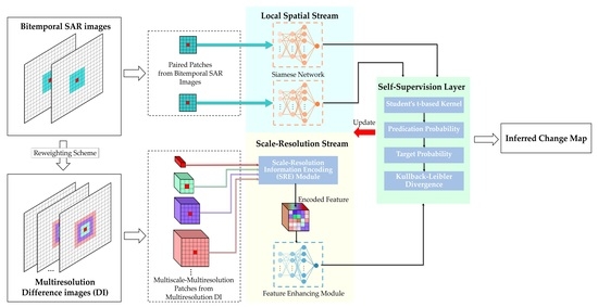
The pipeline of the proposed hybrid variability aware network (HVANet) is graphically illustrated in Figure 4. The whole HVANet consists of two streams (i.e., the local spatial stream and the scale-resolution stream) and a self-supervision layer. The local spatial stream is a Siamese network (SiamNet) that handles the SP part in the ESP feature, while the scale-resolution stream is composed of two modules that are in charge of processing the MS-MR part in the ESP feature. In this way, local structural features and encoded MS-MR features that contribute to the changed region identification are further extracted, following which the self-supervision layer combines the two types of features together into a high-level feature and classifies it. Intrinsically, the HVANet projects the ESP features into a learned high-level feature space, where the features are semantically discriminative and feature classification is easier.
3.3.1. Local Spatial Stream
As shown in Figure 4, the local spatial stream consists of a pair of twin subnetworks with symmetric structure and shared weights, referred to as the Siamese network (SiamNet) [47,48,55]. Unlike the traditional DNN-based methods [30,37], which concatenates the paired patches, i.e., SP, and processes it using a deep network, the two-branch architecture enables the SiamNet to learn respective local structural features from the paired inputs in the same way. Hence, the changed patch pair will have paired features away from each other. Meanwhile, the unchanged patch pair will have pretty similar activations on the corresponding features. Considering that the CD task seeks to measure the dissimilarity between the paired pixels, such a SiamNet architecture is naturally appropriate for further improving the accuracy of change information extraction. Specifically, the SiamNet is composed of fully connected layers, where layer-wise feature extraction can be formulated as
where and denote the bilateral inputs and outputs corresponding to the lth fully connected layer, represent the weights and bias at this layer, and is a nonlinear function. The final outcomes at the fully connected layer are the learned features in the local spatial stream, denoted as for clarity.
Benefiting from the bilateral feature extraction nature of the SiamNet architecture, the fine structure information in and is separately and independently preserved in and , thus promoting better spatial information description.
3.3.2. Scale-Resolution Stream
In the local spatial stream, the patch-wise content primarily influences the local structure feature extraction. However, as SAR images often contain too many changed regions with arbitrary sizes, shapes, and textures, it is still arduous to accurately identify changes of interest using merely the original SP features. To further facilitate the distinguishability of learned high-level features, the scale-resolution stream is appended to compensate for the missing contextual information to cope with the hybrid variabilities.
To fully make use of the MS-MR information to obtain a spatially and semantically powerful feature representation complementary to the structure feature in the local spatial stream, a scale-resolution information encoding module (SRE) is first devised to encode the information in the MS-MR patches. In reality, not all scales or resolutions are equally important for contributing to the CD task. Therefore, channel attention [56] is introduced into SRE to learn what features to highlight; that is, more informative scales and resolutions should be emphasized while secondary ones should be suppressed, thus acquiring an encoded feature. Immediately after the SRE module, an ordinary DNN is attached to extract high-level representation further.
(1)Scale-ResolutionInformationEncoding Module: To concentrate on the task-related features and suppress secondary information automatically, the SRE is proposed. The MS-MR patches in the ESP feature, i.e., , are used as inputs of this module. Specifically, the cross-resolution information encoding unit (CRE) and within-resolution information encoding unit (WRE) are placed in parallel to process the MS-MR input . The CRE is responsible for capturing the informative scale and resolution clues and compressing the secondary information, while WRE is in charge of compensating the necessary spatial content. Later, the features extracted by the two units are aggregated as in channel attention [56] to embrace the key scale and resolution clues and redistribute the change feature representation, finally strengthening the representation ability. The SRE module is illustrated graphically in Figure 5.
The CRE unit contains K-1 convolution branches, each of which is composed of two convolution operations: a depthwise convolution (DWC) [57] and an ordinary convolution. The CRE unit aims to explore the cross-resolution correspondence for each patch feature in to capture the informative scale and resolution clues. Particularly, the patch at the basic scale, i.e., , is utilized as the input of WRE and not involved in this unit. Without loss of generality, we describe the encoding process for the kth feature to illustrate the CRE unit. Specifically, a DWC operation with kernel size 1 × 1 is firstly applied to as
where weight and bias correspond to , denotes a nonlinear activation function, and the symbol represents the DWC operation. Here, the 1 × 1 DWC convolves the input patch channel-by-channel, thus capturing the nonlinear spatial features at each resolution without changing the spatial dimension. Following this, the cross-resolution correspondence is realized through a normal convolution (Conv) with the kernel size , thus learning an importance descriptor of the different resolutions adaptively, as
where denote the weights and biases of the current Conv layer, represent the sigmoid function, and the symbol denotes convolution. Since the regular Conv kernel will fuse the entities across channels, the compressed feature vector is captured by summarizing both the within-resolution and cross-resolution information. Moreover, the importance descriptor of different resolutions can be learned at each scale, which carries both resolution and scale clues.
After extracting importance descriptors at K-1 scales in the CRE unit, most secondary information in is compressed. To compensate for the compressed information, we propose a simple yet effective WRE unit. Specifically, the WRE unit is in charge of processing the unique feature at the basic scale bs (), of which the height and width are the same as the SP feature . This unit encodes the internal change information at each resolution in without any cross-resolution correspondence by sequentially using two learnable 1 × 1 DWC layers, as
where and denote the weights and biases of the two 1 × 1 DWC layers, respectively, and , are the corresponding outputs. Relying on the depthwise operation nature that employs a single convolutional filter per input channel, dimension-invariant nonlinear transformation is realized using the 1 × 1 DWC kernels, and internal spatial information at different resolutions can be separately preserved.
To embrace the different scale clues and focus on the informative resolutions simultaneously, it is a natural belief that the learned importance descriptors at different scales in CRE should be fully combined and then weight the extracted features in WRE; thus, the scale, resolution, and spatial information can be harmoniously integrated together. To this end, the features and are aggregated as in the channel attention mechanism [56]. Formally,
where the symbol denotes the element-wise product and is the integrated importance descriptor. Particularly, refers to the channel-wise product between and , and its output is the final encoded features, where the whole MS-MR information is selectively and automatically summarized. As described earlier, the SRE module intrinsically performs the channel-wise attention, which jointly emphasizes the features from informative resolutions and scales according to the learned importance descriptors and promotes the feature learning to be aware of the variable size and texture characteristics.
(2) FeatureEnhancing Module: Immediately after the SRE module, a regular DNN is utilized as a feature extractor to learn high-level features to enhance the representation power, called the feature enhancing module (FE), which has the same architecture as the two branches of SiamNet. This module learns an adaptive mapping function that takes the encoded feature as the input and generates the high-level feature , namely the final outcome of the scale-resolution stream.
3.3.3. Greedy Layer-Wise Unsupervised Pretraining
The direct application of self-supervised learning is very challenging given the high dimensionality of the ESP features. To better initialize the network weights and capture some useful features, we propose to adopt greedy layer-wise unsupervised pretraining [58,59,60]. Specifically, the SiamNet in the local spatial stream and the FE module in the scale-resolution stream are individually pretrained.
Considering the specific architecture of the SiamNet, we design a symmetric layer-wise pretraining strategy to promote the target-specific feature learning. Specifically, the initial weight matrix and bias vector of the lth layer in SiamNet is learned through a specially designed Siamese autoencoder (SiamAE) with a single hidden layer. For the lth layer in SiamNet, the corresponding SiamAE can be formulated as
where , , and denote the input, hidden representation, and output of the SiamAE. and represent the weight matrix and bias vector of the encoder and decoder in the SiamAE, respectively. The input of the first layer is the SP feature; i.e., . Finally, initialization is achieved by minimizing the L2 norm of the difference between and :
After being pretrained by this strategy, the weights and biases of the lth layer will be kept unchanged in the pretraining stage. With the symmetric layer-wise pretraining strategy that enforces the SiamAE to reconstruct the SP feature, the SiamNet in the local spatial stream is encouraged to extract some useful features to provide a better parameter initialization.
Similar to the symmetric layer-wise pretraining described above, the pretraining strategy for the lth layer of the FE module in the scale-resolution stream can be summarized as follows:
Here, the input of the first layer is in the ESP feature. As such, the FE module is pretrained layer-by-layer. By means of the pretraining strategy, most network weights in HVANet can be well initialized. Since the multi-branch architecture of the SRE module in the scale-resolution stream cannot be pretrained in such a layer-wise way, weights in the SRE are initialized using the technique described in [61].
3.3.4. Self-Supervised Fine-Tuning
(1) Self-supervision Layer: Due to the lack of ground truth labels in SAR data, training targets are not available for unsupervised learning. As a result, it is necessary to explore how to eliminate the requirement of labeled data by creating learning signals for model training. To this end, a specialized self-supervision layer is constructed to allow performing feature classification and providing learning signals for fine-tuning simultaneously, which is inspired by the deep embedded clustering method [62].
Specifically, given the training set , the two streams in HVANet can extract three features for each input. The self-supervision layer combines them together to form a united feature, as , under which the two streams are also united into one framework. Later, we compute the initial class centers by performing k-means on , where subscript “0” represents the unchanged class and “1” represents the changed class. These initial class centers will provide an approximate optimization direction and enable the later learning process, namely the self-supervision.
We calculate the probability that the ith input sample is assigned to the jth class by measuring the similarity between and based on a Student’s t-distribution-based kernel [62], as
where is the united high-level feature corresponding to the ith input . The rationale behind the probability calculation is to use the Student’s t-distribution as a kernel to transform the similarity of a feature to a certain class center into the class probability. In this regard, the heavy-tailed property of the Student’s t-distribution is powerful for robustly fitting and describing the feature distribution in the high-level feature space. In addition, beyond the initial class centers that are calculated by directly performing k-means on H, the class centers can be updated automatically in training, as further described in the following subsections.
It is intuitive that the inputs with high confidence could provide more reliable class knowledge and be utilized as learning signals to guide the network fine-tuning in a self-supervised manner. In this direction, the supervision signal is constructed by raising to the second power to emphasize the reliable class knowledge, as
where is the soft frequency of the jth class and is the newly created supervision signal for the ith input feature. The soft frequency helps to normalize the contribution of each training sample, such that class imbalance can be further alleviated.
The supervision signal is completely generated from the probability but with reduced entropy since it is calculated by raising to the second power. Consequently, the training target is constructed by paying attention to the credible unlabeled samples with high predicated class probability, the so-called self-supervision.
(2) Self-supervision Loss: To progressively force the model to learn with useful class knowledge from unlabeled features themselves, the training target is constructed and can provide a meaningful optimization objective for the fine-tuning of HVANet. Using such a self-supervision strategy, the HVANet is encouraged to output low-entropy (i.e., highly confident) predictions and progressively achieve entropy minimization. Following this idea, a Kullback–Leibler (KL) divergence-based loss function is adopted to quantify the similarity between the predicted distribution Q and the target distribution P, as
Herein, KL divergence between distributions Q and P is adopted as an objective for network optimization. Minimizing the objective function encourages the similar features to cluster together while separating the dissimilar features in the learned high-level space, such that the classification in the feature space becomes easier.
(3) Optimization: To effectively fine-tune the HVANet in a completely unsupervised manner, both the network weights and class centers should be updated with back propagation based on the self-supervised loss . The optimization can be formulated as
where denotes the learning rate. The update of class centers provides the optimization direction for the next training epoch. More importantly, the repeated update of network weights encourages HVANet to learn useful class knowledge from unlabeled samples and promote the model performance progressively.
3.3.5. Computational Complexity Analysis
Here, we provide a rough evaluation on the computational complexity of the HVANet. To be specific, the computational cost of each training epoch comes mainly from calculating features in the local spatial stream and calculating feature in the scale-resolution stream. Hence, in this section, we analyze the computational complexity of the HVANet, given n input ESP features .
In the training of the local spatial stream, the n pairs of patches are fed into the first layer with neutrons. For each output neuron at the first fully connected layer, when one flattened image patch is fed, there are multiplications between weights and inputs and additions to sum the multiplication results and bias. As the nonlinear activation function is applied to the outputs of the fully connected layers, the computational complexity of the utilized nonlinear function should be considered, which is denoted as floating point operations (flops) for the sake of clarity. Therefore, there are flops for a pair of input patches . Similarly, the next fully connected layer has flops. In this way, for the SiamNet in the local spatial stream which has fully connected layers, the total number of flops (abbreviated as ) can be formulated as
Hence, the computational complexity of the local spatial stream at each training epoch can be represented as flops.
As for the scale-resolution stream, both the computational complexities of the SRE module and the FE module should be considered, respectively. As the elaboration in Section 3.3.2, when n MS-MR patch features are fed into the SRE module, the CRE unit processes the features while the WRE unit processes the feature . On the one hand, the CRE unit contains branches, each of which successively performs the DWC and an ordinary convolution operation. For the kth branch in the CRE unit, the corresponding input feature is processed using a DWC operation with kernel size , which involves multiplications for the combination between the kernel and input, and additions between the combination and bias. Since each pixel in the feature map of DWC should be processed by the nonlinear function, the resulting computational complexity is flops. Later, when the activated output is fed into an ordinary Conv layer with kernel size , there are multiplications and additions. Besides, there is an additional computational complexity caused by the nonlinear function. Thus, the total computational complexity of the branches in the CRE unit can be summarized as flops. On the other hand, the WRE unit processes the using two successive DWC operations with kernel size , which involves multiplications, additions. Two nonlinear functions also cause flops. For the feature aggregation in CRE, the integration of the learned importance descriptors involves multiplications and channel-wise attention requires multiplications. Finally, the encoded feature is fed into the FE module, which has an identical network architecture to the SiamNet, but the dimension number of the input layer is . In summary, the total number of flops of the scale-resolution stream (abbreviated as ) can be summarized as
Consequently, given n input ESP features , the computational complexity of the entire HVANet at each training epoch can be represented as flops.
According to the above analysis, the main computational cost comes from the SiamNet in the local spatial stream and the FE module in the scale-resolution stream, where the fully connected layers account for most parameters in HVANet. By contrast, we introduce the channel-wise attention and the DWC operation for the MS-MR information encoding in the SRE module, enabling effective feature extraction with negligible computation cost. Moreover, the small sizes of the patches in the ESP feature determine that the scale of the utilized fully connected layers and the corresponding computational complexity is relatively limited, which means the HVANet is lightweight and efficient in the training phase and inference phase. To further illustrate the computational complexity of the HVANet, we compare the training time and inference time of the HVANet with other unsupervised CD methods in Section 4.
4. Experimental Results
In this section, we performed extensive experiments to ensure that the entire proposed CD system is effective. Experiments were conducted on three real datasets. We compare the proposed HVANet with some state-of-the-art methods in terms of objective indexes and visual results. Our experiments were conducted on a workstation with an Intel(R) Core(TM) i7-8750H CPU (6 cores, 2.2 GHz, 32 GB RAM) and an Nvidia Quadro P2000 graphical processing unit (GPU) (4 GB RAM). Particularly, the proposed HVANet was implemented using the Keras with the TensorFlow backend [63] and MATLAB 2016a in Windows 10 environment. The corresponding code of the proposed method will be made available at https://github.com/CATJianWang/HVANet (accessed on 16 December 2021).
4.1. Dataset Description
The proposed HVANet method was conducted on three representative bitemporal SAR image datasets: the Ottawa dataset, the Farmland A dataset, and the Farmland B dataset. The corresponding real SAR images and ground truth maps for three datasets are shown in Figure 6, Figure 7 and Figure 8. More detailed introductions of three datasets are provided as follows.
- 1.
- Ottawa dataset: Ottawa dataset was captured by Radarsat-1 in July and August 1997, respectively. The images in this dataset have a low spatial resolution with a spatial size of 290 × 350. Figure 6a,b show the bitemporal SAR images and Figure 6c shows the corresponding ground truth map. The dataset reflects the flooded areas over Ottawa, Canada.
- 2.
- Farmland A dataset: Farmland A dataset was acquired in June 2008 and June 2009 by the Radarsat-2 sensor over an agricultural area at the Yellow River Estuary in China. The SAR images have a higher spatial resolution than Ottawa dataset, which covers an area with 289 × 257 pixels and has a spatial resolution of 3 m. The SAR images and the ground truth map are shown in Figure 7. The changed parts are mainly caused by the cultivation.
- 3.
- Farmland B dataset: Farmland B dataset was collected in June 2008 and June 2009 by the Radarsat-2 sensor over an agricultural area at the Yellow River Estuary in China. This dataset covers an area with 291 × 306 pixels, which is characterized by a spatial resolution of 3 m. In common with Farmland A, this dataset includes the farmland change arising from cultivation. The SAR images and the ground truth map are shown in Figure 8.
Particularly, in the last two datasets, the SAR images acquired in June 2008 are four-look, but the images obtained in June 2009 are single-look, indicating a significant discrepancy of the impact of speckle noise on the bitemporal images. Obviously, such a discrepancy would increase the difficulty of CD in these two datasets. Furthermore, these bitemporal SAR image datasets are publicly available for download at https://github.com/CATJianWang/HVANet/tree/main/Dataset (accessed on 16 December 2021).
4.2. Experimental Settings
(1) Evaluation Criteria: Both visually qualitative comparison and quantitative measures are applied to evaluate the results of the proposed method and competing methods. On the one hand, change detection results are shown in an intuitively visual way, namely the binary change map. On the other hand, false positives (FP), false negatives (FN), overall errors (OE), percentage of correct classification (PCC), and Kappa coefficient (κ) are employed as the evaluation criteria. FP is the number of unchanged pixels that are wrongly detected as changed pixels, whereas FN is the number of changed pixels that are wrongly detected as unchanged pixels. OE is the sum of FP and FN, representing the total number of misclassified pixels. Moreover, PCC is computed as
Kappa (κ) is calculated as below:
where
Here, TP (abbreviation for true positives) denotes the number of changed pixels that are correctly detected as the changed class, while TN (abbreviated for true negatives) represents the number of unchanged pixels that are correctly detected as the unchanged class. Note that the provided experimental results below are the mean criteria values after running 10 times.
(2) Network Architecture: To accomplish the network training and testing with high effectiveness and efficiency, the HVANet architecture is made to be lightweight, reducing network parameters and speeding up network operation. The detailed structure of the HVANet is shown in Table 1. During training, we employ the stochastic gradient descent (SGD) optimizer to train the network and set the learning rate to 0.0001, batch size to 128, and momentum to 0.9.
4.3. Ablation Study
To better understand HVANet, we conducted an ablation study to show the effectiveness of our model components, including the local spatial stream (abbreviated as LSS in this section), the scale-resolution stream (abbreviated as SRS in this section), and the SRE module in the SRS. Besides, the effect of the proposed class rebalance strategy is also studied to illustrate its role in the construction of the training set and then the model training.
(1)Contribution of Local Structure Information Extraction in LSS: From the perspective of the SiamNet architecture in the LSS, local structure information in bitemporal images can be preserved and extracted independently. For comparison, only fully connected layers are considered to replace the Siamese architecture in HVANet. Specifically, we compare the HVANet (LSS + SRS) and regular DNN + SRS while the network architecture in SRS is kept the same for these two models. Here, the input of the regular DNN is the concatenation of the vectorized SP feature , . Besides, we also perform the comparison between the LSS (SiamNet) and regular DNN without SRS to further show the superiority of the SiamNet in extracting change information. Comparing the two feature extraction architectures, regular DNN does not perform well because the structural information independently inherited from two patches is destroyed and the extracted features are not effective. The ablation study results are reported in Table 2. Benefiting from the structure-preserved nature, LSS (SiamNet) can effectively capture the high-level structural features by learning, achieving better performance.
(2) Contribution of Scale-Resolution Information Encoding in SRS: To investigate the important role played by the scale-resolution stream in the CD performance, we conduct ablation on SRS. Specifically, there are two ablation strategies: (1) removing the entire SRS from HVANet and the resulting model, i.e., the LSS (SiamNet), is compared with the HVANet to verify the efficiency of SRS; (2) removing the SRE module while retaining the feature enhancing (FE) module in SRS to further validate the effectiveness of the ability of scale-resolution information encoding of SRE module. As shown in Table 3, the models HVANet (w/o SRS) and HVANet (w/o SRE) receive significant drops in PCC and Kappa. The results indicate that the SRS is critical in our HVANet, especially the SRE module that can fully exploit MS-MR information and capture the informative scale and resolution clues to strengthen the description of the hybrid variabilities in CD scenes. Furthermore, despite the fact that the structural information extracted in LSS (SiamNet) can improve the description at each pixel, the distinguishable and generalizable information is still scarce such that the category knowledge learning remains a tough task, restricting the model performance. On the contrary, our model can make full use of both structural information and MS-MR information and aggregate them, thus can obtain a semantically discriminative feature. This also indicates that the MS-MR information is of great significance in providing useful feature representations.
(3) Effect of Class Rebalance Strategy: The proposed HVANet is intrinsically a data-driven model that relies strongly on the training samples. The imbalance of the samples of different categories inevitably has a negative impact on the training efficiency. In this context, we specially designed the class rebalance strategy to mitigate the imbalance, which is a challenging problem in SAR image CD, especially when the ground truth or real labels are unavailable. We performed ablations on the strategy. We set the HVANet trained with the samples selected by regular k-means clustering as the baseline (i.e., replacing the hierarchical clustering in Algorithm 1 and only using the k-means results for the training sample selection). As shown in Table 4, the HVANet can achieve significant improvements in the PCC and Kappa values on the Farmland A dataset when applying the rebalance strategy. This is because the k-means clustering is very susceptible to the speckle noise, intensity fluctuations and pseudochanges, and cannot obtain a relatively accurate result. Hence, the balance in the selected training samples cannot be reached. Therefore, we apply the designed class rebalance strategy to sample the training pixels from the entire images to realize a manageable balance in the training set.
4.4. Parameter Analysis
(1) Number of Considered Scales: The ESP features contain multiscale information at each pixel to enrich the spatial context. Our intuition is that each pixel position of the bitemporal images can be characterized by information at multiple scales and different resolutions, that is the ESP features. In this way, the number of considered scales K is a significant hyperparameter. We test different to investigate its effect on the performance of the HVANet using the Ottawa, Farmland A, and Farmland B datasets. As shown in Table 5, for Ottawa and Farmland A datasets, our model achieves the best performance when increasing K from 1 to 3; for the Farmland B dataset, the best performance is obtained under . It can be observed that the model encounters a performance drop when decreasing K from 3 to 1. This is because the small scales, e.g., 1 × 1 and 3 × 3, lack spatial neighbor information to produce semantically strong features, resulting in many incorrectly detected pixels. Although there are performance improvements by further increasing the number of scales on Farmland B, for the consistency and the tradeoff between efficiency and precision, we set K to 3 in the following experiments.
(2) Basic Scale: For the proposed method, the basic scale (i.e., patch size height × width) , which determines the size of input patches of the HVANet, influences the final change detection result. Intuitively, a larger B indicates that more local information is considered and therefore tends to produce a semantically smoother change map. Nevertheless, the image details may be lost under an overly large B. In contrast, a smaller B is beneficial to preserve the delicate details and local structures but is sensitive to the extensive speckle noise in SAR images. For this reason, parameter B is analyzed using three datasets. Table 6 reports the results obtained by HVANet on three datasets under different values of size B. As can be seen, the best performance is achieved when a small patch size ( for Ottawa dataset and for Farmland A and Farmland B datasets) is employed, while enlarging the patch size only decreases the PCC and Kappa values. This is because the small patch size effectively preserves the detailed structural information in the local spatial stream, while the scale-resolution stream helps to compensate for the context information from MS-MR change information to deal with the hybrid variabilities in SAR imagery. The large patch size will cause that fine structural information cannot be emphasized. As a result, we set the patch size to be , , and for the Ottawa, Farmland A, and Farmland B datasets, respectively.
(3) Number of Resolutions: The number of resolutions L is a significant hyperparameter. We study the performance of the HVANet with different configurations of the input ESP features that contain different numbers of resolution levels, i.e., . Table 7 exhibits significant improvements in the PCC and Kappa values of our model on the three SAR image datasets when increasing the number of resolution levels. These results indicate that more resolution levels could enrich the context information to better characterize the change information at each pixel and make the constructed ESP features more discriminative and generalizable. Consequently, we set the number of resolution levels L to 5.
4.5. Visualization of the Learned High-Level Features
To intuitively demonstrate the discriminative power of HVANet, we adopt the t-SNE [64] to visualize the initial ESP features and the learned united features at each pixel position in the bitemporal images extracted by using the HVANet after self-supervised learning, respectively, as shown in Figure 9. It can be seen in the first row of Figure 9 that the samples from change and non-change classes severely overlap with each other in the feature space. This indicates that speckle, pseudochanges, and hybrid variabilities have a significant influence on the shallow ESP features, which are not suitable for identifying changes. Meanwhile, the high-level features learned by HVANet in the self-supervised learning manner exhibit larger inter-class separability and intra-class compactness. Moreover, the self-supervised learning framework can effectively discover and exploit category knowledge in unlabeled samples and learn a new high-level feature space, where the margin between the features of change and unchanged classes is enlarged, indicating that feature classification becomes easier.
4.6. Comparison to Counterpart Methods
We make a comparison to several existing unsupervised SAR CD methods, including two typical clustering-based methods (PCA-kmeans [17], GaborTLC [18]), and five unsupervised deep learning-based methods (PCANet [38], DDNet [40], CWNN [39], INLPG-CWNN [20], and SGDNNs [30]).
- 1.
- 2.
- 3.
- PCANet [38]: A deep learning-based method under a preclassification scheme. Gabor wavelet [66] is used to extract shallow features, to which a clustering algorithm is applied for the generation of pseudolabeled samples; thus, the training of the PCANet can be performed using the pseudolabeled samples.
- 4.
- DDNet [40]: Frequency and spatial domain-based method under a preclassification scheme, where features of frequency and spatial domains are integrated using two modules to improve the representation power of learned features.
- 5.
- 6.
- 7.
- SGDNNs [30]: Saliency-guided preclassification-based method, which combines the saliency map and the log-ratio DI into a fused DI, and hierarchical clustering is applied to the combined DI for the acquisition of pseudolabeled samples. A DNN is optimized using the pseudo labeled samples for the CD task.
We implement these methods using their publicly available codes and default settings.
The experimental results on the Ottawa dataset are reported in Table 8. As we can see, the two traditional methods, PCA-kmeans and GaborTLC, obtain inferior statistical value results because the handcrafted features cannot well characterize the hybrid variabilities in SAR images and the typical clustering algorithms lack an adequate ability to fit the complex SAR data. By contrast, the deep learning-based methods, including the PCANet, DDNet, CWNN, SGDNNs, and our HVANet, produce better results due to the powerful feature learning capability from deep models. Particularly, the SGDNNs achieve the best performance in this dataset, i.e., the largest PCC (98.95%) and Kappa value (95.94%). It is observed that our HVANet model obtains comparable PCC (98.59%) and Kappa values (94.64%) with the SGDNNs.
Change detection maps are shown in Figure 10. As shown in Figure 10a,b, the conventional clustering-based methods often confuse unchanged pixels with changed pixels. Meanwhile, deep learning-based methods better infer and separate the changed and unchanged classes, as shown in Figure 10c–h. It is observed that SGDNNs outperform other competing methods, produce the lowest false alarms, and retain more details, as shown in Figure 10g. Regarding our HVANet, even though some isolated pixels are not well processed in the result, the visual effect of HVANet is quite comparable with the result of SGDNNs. Moreover, the results shown in Figure 10 are consistent with those listed in Table 8.
The change maps from different methods and the corresponding statistical values on the Farmland A dataset are reported in Table 9 and shown in Figure 11, respectively. According to the introduction in Section 4.1, the Farmland A and Farmland B datasets seriously suffer from speckle noise, which easily causes poor results. According to the reported results in Table 9 and Figure 11, the traditional methods, PCA-kmeans and GaborTLC, show inferior results that contain extensive incorrectly detected isolated regions and pixels. Similarly, due to the complex scene and hybrid variabilities, the two deep learning-based methods, i.e., INLPG-CWNN and SGDNNs, encounter high FN values. However, Figure 11c–e visually exhibit better detection results, demonstrating that the PCANet, DDNet, and CWNN methods are suitable for this data set. Particularly, the CWNN returns the best results with the highest PCC (96.60%) and Kappa values (88.23%). Our proposed HVANet achieves comparable results from the perspective of the statistical values and visual effect. More importantly, the post-processing operation is adopted in PCANet [38] to eliminate the isolated regions that are likely to be false alarms, while the similar operation is unnecessary and not utilized in our method. Besides, according to the visual results in Figure 11, the change maps inferred by the HVANet are more complete and have better consistency compared with other change maps. Particularly, benefiting from the structural information extraction and the scale-resolution awareness of HVANet, the strip changed regions are detected while the hard-to-classify pixels are well processed. In summary, for this dataset, the proposed method significantly exceeds most unsupervised SAR image CD approaches, including traditional and recently proposed deep learning-based.
Figure 12 shows the change detection results on the Farmland B dataset. The corresponding evaluation metrics are listed in Table 10. PCA-kmeans and GaborTLC suffer from high FP values, which indicates that the speckle noise and pseudochanges severely affect the performance of conventional clustering algorithms. Similar to the results on the first two datasets, the deep learning-based methods perform better than the conventional methods on this dataset. It should be noted that our HVANet achieves the best performance and produces the best change map, which is closer to the ground truth map. Concretely, in the change map shown in Figure 12h, fewer pixels are incorrectly detected and the details in changed regions are completely preserved, which demonstrates the effectiveness of the high-level feature learning in HVANet.
From the experimental results, it can be concluded that the proposed HVANet is effective for CD on bitemporal SAR images. To further illustrate the superiority of HVANet, the average values of all the evaluation criteria on three different datasets are calculated, as listed in Table 11. It is observed that HVANet provides the highest average PCC (97.96%) and Kappa value (90.82%), which illustrates that HVANet achieves better CD results and is more robust than the competing methods. That is to say, compared with the other methods, HVANet can provide relatively stable and credible CD results, which are meaningful in practical applications that may encounter different scenes and data distributions. Consequently, as a tradeoff between performance and stability, HVANet is a suitable and useful model for SAR image CD.
4.7. Computational Efficiency
In this section, the computational efficiency of different SAR image CD methods is reported. Among the compared methods, PCA-kmeans and GaborTLC are the traditional clustering-based methods that can directly perform prediction for the given SAR images without training. PCANet, DDNet, and CWNN are all deep learning-based unsupervised methods, where model training is necessary to achieve good CD performance. Particularly, for the deep learning algorithms, training time and inference time rely strongly on the hyperparameter setting and running environments. Therefore, this paper uses the default setting of the compared methods to count the training time and inference time. Table 12 reports the training time and inference time of these methods. As can be seen from Table 12, the traditional CD methods, i.e., PCA-kmeans and GaborTLC, have a significant time advantage because there is no training procedure. Despite the training procedure of deep learning models bringing more computational time, the inference speed is relatively fast and the total inference time is short. Furthermore, HVANet does not have an advantage in training time due to its more complex network architecture. Compared with the deep learning-based methods, i.e., PCANet, DDNet, and CWNN, the proposed HVANet spends less inference time on the Ottawa dataset and Farmland A dataset, while the inference time of HVANet on the Farmland B dataset is moderate. Considering the tradeoff between computational cost and the detection accuracy, HVANet is more suitable for the CD task for SAR images.
5. Discussion
The experimental results are provided in Section 4 and illustrate that the proposed label-free method achieves better and more robust CD performance for SAR images than the competing methods. The reason why the proposed method surpasses the compared state-of-the-art methods resides in three aspects. One is that, inspired by the human perception mechanism that processes local and global information independently, we construct the shallow feature by combining the local patches and context-rich MS-MR patches, displacing the traditional single-scale processing unit. The context information and diverse scale and resolution information contained in the constructed ESP features are conducive to improving the description for change information and making it more differentiated from the speckle and pseudochanges. The second reason lies in the two-stream feature extraction in HVANet, which combines the local spatial feature extraction and MS-MR information encoding into one framework, improving the representation power of the learned high-level features. Particularly, the channel attention mechanism is adopted in the scale-resolution stream to effectively aggregate the key multiscale clues and multiresolution clues for better feature representation. Third, the self-supervision layer enables the feature learning and classification to be automatic, end-to-end, and label-free. Despite real labels and the corresponding class knowledge being unavailable, the performance of our HVANet matches or exceeds that of the compared state-of-the-art methods.
From the ablation experiments in Section 4.3, we illustrate the contribution of each component in HVANet and the class rebalance strategy. In Table 2, the results show that the Siamese structure is naturally more suitable for CD tasks due to the separate processing of the SAR image patch pair. As in Table 3, the results show that the scale-resolution stream really extracts semantically distinguishable features that can greatly enhance the description of change information, thus improving the detection accuracy. For the hybrid variations of sizes, shapes, and textures in changed regions, the scale-resolution can better model them and intensify the robustness of the CD system. The main reason is that not only can the deep architecture process the complex SAR data in a nonlinear way, but also local features and contextual semantic features can be extracted in the two streams of HVANet to contribute to the CD tasks. Meanwhile, the class imbalance in SAR data also poses challenges for CD tasks. For this, we propose the class rebalance strategy to redistribute the training samples to achieve a balanced class distribution in the training set. The results in Table 4 demonstrate that the proposed hierarchal clustering-based strategy can provide better results than ordinary k-means clustering. Moreover, the deep learning-based competing methods, including PCANet, DDNet, CWNN, INLPG-CWNN, and SGDNNs, neglect this problem, where the distribution of the constructed training set is severely imbalanced. According to the results in Table 8, Table 9, Table 10 and Table 11 and Figure 10, Figure 11 and Figure 12, the detection performance of these methods is unstable, which more or less reflects the negative impact of the class imbalance on the model performance.
According to the experimental results in Section 4.6, we can conclude that the proposed method matches or even exceeds the competing methods from the perspectives of performance, generalization, and robustness. It can be seen from Figure 10, Figure 11 and Figure 12 that the results of the proposed methods are closer to the ground truth map, with fewer false positive and false negative pixels. The same conclusion can also be made from the evaluation criteria provided in Table 8, Table 9, Table 10 and Table 11. Accordingly, all these results confirm that both local structure information and the context-rich MS-MR information help to jointly retrieve more details and suppress speckle and pseudochanges, meaning that the shallow feature extraction and the corresponding two-stream network architecture are obviously suitable for the CD tasks in SAR imagery.
6. Conclusions
In this paper, considering the hybrid variabilities in bitemporal SAR images, which significantly complicate the CD task, we formulated a novel self-supervised framework to learn a semantically powerful high-level feature for label-free SAR image CD. The proposed HVANet contains two separate streams in the feature extraction stage, one of which takes advantage of the Siamese network architecture to extract local structural features from the bitemporal SAR images and the other utilizes the carefully devised SRE module to capture the informative scale and resolution features to enhance the representation power further. More importantly, the self-supervision layer is introduced to aggregate the above-mentioned two types of features to reflect change information effectively and comprehensively, and it could also unify the two streams into one framework for end-to-end self-supervised learning. The experimental results based on the Ottawa dataset, Farmland A dataset, and Farmland B dataset demonstrate that the proposed HVANet outperforms some conventional CD methods and other state-of-the-art deep learning-based CD methods, exhibiting its superiority.
Even though the proposed CD method provides a significant performance improvement, how to learn sufficiently accurate category information from unlabeled data in an unsupervised manner is still a challenging problem in the field of SAR image CD. In the future, we will further focus on unsupervised information extraction and classification with novel deep learning technologies.
Author Contributions
Conceptualization, J.W.; methodology, J.W.; software, J.W.; validation, J.W.; writing—original draft preparation, J.W.; writing—review and editing, J.W. and Y.W.; visualization, J.W.; supervision, Y.W. and H.L. All authors have read and agreed to the published version of the manuscript.
Funding
This work was supported in part by the National Natural Science Foundation of China under Grant 61671354, in part by the 111 Project, and in part by the Shaanxi Innovation Team Project.
Institutional Review Board Statement
Not applicable.
Informed Consent Statement
Not applicable.
Data Availability Statement
Not applicable.
Acknowledgments
The authors would like to thank all reviewers and editors for their comments on this paper.
Conflicts of Interest
The authors declare no conflict of interest.
References
- Radke, R.J.; Andra, S.; Al-Kofahi, O.; Roysam, B. Image change detection algorithms: A systematic survey. IEEE Trans. Image Process. 2005, 14, 294–307. [Google Scholar] [CrossRef] [PubMed]
- Shi, W.; Zhang, M.; Zhang, R.; Chen, S.; Zhan, Z. Change detection based on artificial intelligence: State-of-the-art and challenges. Remote Sens. 2020, 12, 1688. [Google Scholar] [CrossRef]
- Bovolo, F.; Bruzzone, L. The time variable in data fusion: A change detection perspective. IEEE Geosci. Remote Sens. Mag. 2015, 3, 8–26. [Google Scholar] [CrossRef]
- Bovolo, F.; Bruzzone, L. A detail-preserving scale-driven approach to change detection in multitemporal SAR images. IEEE Trans. Geosci. Remote Sens. 2005, 43, 2963–2972. [Google Scholar] [CrossRef]
- Liu, J.G.; Black, A.; Lee, H.; Hanaizumi, H.; Moore, J.M. Land surface change detection in a desert area in Algeria using multitemporal ERS SAR coherence images. Int. J. Remote Sens. 2001, 22, 2463–2477. [Google Scholar] [CrossRef]
- Bruzzone, L.; Serpico, S.B. An iterative technique for the detection of land-cover transitions in multitemporal remote-sensing images. IEEE Trans. Geosci. Remote Sens. 1997, 35, 2963–2972. [Google Scholar] [CrossRef] [Green Version]
- Burnner, D.; Lemonie, G.; Bruzzone, L. Earthquake damage assessment of buildings using VHR optical and SAR imagery. IEEE Trans. Geosci. Remote Sens. 2010, 48, 858–867. [Google Scholar] [CrossRef] [Green Version]
- Coca, M.; Anghel, A.; Datcu, M. Unbiased seamless SAR image change detection based on normalized compression distance. IEEE J. Sel. Topics Appl. Earth Observ. Remote Sens. 2019, 12, 2088–2096. [Google Scholar] [CrossRef]
- Sun, Y.; Lei, L.; Guan, D.; Li, X.; Kuang, G. SAR image change detection based on nonlocal low-rank model and two-level clustering. IEEE J. Sel. Topics Appl. Earth Observ. Remote Sens. 2020, 13, 293–306. [Google Scholar] [CrossRef]
- Oliver, C.; Quegan, S. Understanding Synthetic Aperture Radar Images; Artech House: Boston, MA, USA, 1998. [Google Scholar]
- Saha, S.; Bovolo, F.; Bruzzone, L. Building change detection in VHR SAR images via unsupervised deep transcoding. IEEE Trans. Geosci. Remote Sens. 2021, 59, 1917–1929. [Google Scholar] [CrossRef]
- Moser, G.; Serpico, S.B. Unsupervised change detection from multichannel SAR data by Markovian data fusion. IEEE Trans. Geosci. Remote Sens. 2009, 47, 2114–2128. [Google Scholar] [CrossRef]
- Wang, R.; Zhang, J.; Chen, J.; Jiao, L.; Wang, M. Imbalanced learning-based automatic SAR images change detection by morphologically supervised PCA-Net. IEEE Geosci. Remote Sens. Lett. 2019, 16, 554–558. [Google Scholar] [CrossRef] [Green Version]
- Carincotte, C.; Derrode, S.; Bourennane, S. Unsupervised change detection on SAR images using fuzzy hidden Markov chains. IEEE Trans. Geosci. Remote Sens. 2006, 44, 432–441. [Google Scholar] [CrossRef]
- Aiazzi, B.; Alparone, L.; Baronti, S.; Garzelli, A.; Zoppetti, C. Nonparametric change detection in multitemporal SAR images based on mean-shift clustering. IEEE Trans. Geosci. Remote Sens. 2013, 51, 2022–2031. [Google Scholar] [CrossRef]
- Bazi, Y.; Bruzzone, L.; Melgani, F. An unsupervised approach based on the generalized Gaussian model to automatic change detection in multitemporal SAR images. IEEE Trans. Geosci. Remote Sens. 2005, 43, 874–887. [Google Scholar] [CrossRef] [Green Version]
- Celik, T. Unsupervised change detection in satellite images using principal component analysis and k-means clustering. IEEE Geosci. Remote Sens. Lett. 2009, 6, 772–776. [Google Scholar] [CrossRef]
- Li, H.-C.; Celik, T.; Longbotham, N.; Emery, W.J. Gabor feature based unsupervised change detection of multitemporal SAR images based on two-level clustering. IEEE Geosci. Remote Sens. Lett. 2015, 12, 2458–2462. [Google Scholar]
- Li, L.; Zhao, Y.; Sun, J.; Stolkin, R.; Pan, Q.; Chan, J.C.-W.; Kong, S.G.; Liu, Z. Deformable dictionary learning for SAR image change detection. IEEE Trans. Geosci. Remote Sens. 2018, 56, 4605–4617. [Google Scholar] [CrossRef]
- Sun, Y.; Lei, L.; Li, X.; Tang, X.; Kuang, G. Structure consistency-based graph for unsupervised change detection with homogeneous and heterogeneous remote sensing images. IEEE Trans. Geosci. Remote Sens. 2022, 60, 4700221. [Google Scholar] [CrossRef]
- Rignot, E.M.J.; Van Zyl, J.J. Change detection techniques for ERS-1 SAR data. IEEE Trans. Geosci. Remote Sens. 1993, 31, 896–906. [Google Scholar] [CrossRef] [Green Version]
- Celik, T. Multiscale change detection in multitemporal satellite images. IEEE Geosci. Remote Sens. Lett. 2009, 6, 820–824. [Google Scholar] [CrossRef]
- Celik, T.; Ma, K. Multitemporal image change detection using undecimated discrete wavelet transform and active contours. IEEE Trans. Geosci. Remote Sens. 2011, 49, 706–716. [Google Scholar] [CrossRef]
- Inglada, J.; Mercier, G. A new statistical similarity measure for change detection in multitemporal SAR images and its extension to multiscale change analysis. IEEE Trans. Geosci. Remote Sens. 2007, 45, 1432–1445. [Google Scholar] [CrossRef] [Green Version]
- Bruzzone, L.; Prieto, D.F. Automatic analysis of the difference image for unsupervised change detection. IEEE Trans. Geosci. Remote Sens. 2000, 38, 1170–1182. [Google Scholar] [CrossRef] [Green Version]
- Xiong, B.; Chen, Q.; Jiang, Y.; Kuang, G. A threshold selection method using two SAR change detection measures based on the Markov random field model. IEEE Geosci. Remote Sens. Lett. 2012, 9, 287–291. [Google Scholar] [CrossRef]
- Carotenuto, V.; Maio, A.; Clemente, C.; Soraghan, J. Unstructured versus structured GLRT for multipolarization SAR change detection. IEEE Geosci. Remote Sens. Lett. 2005, 12, 1665–1669. [Google Scholar] [CrossRef] [Green Version]
- Gong, M.; Zhou, Z.; Ma, J. Change detection in synthetic aperture radar images based on image fusion and fuzzy clustering. IEEE Trans. Image Process. 2012, 21, 2141–2151. [Google Scholar] [CrossRef]
- Celik, T.; Ma, K. Unsupervised change detection for satellite images using dual-tree complex wavelet transform. IEEE Trans. Geosci. Remote Sens. 2010, 48, 1199–1210. [Google Scholar] [CrossRef]
- Geng, J.; Ma, X.; Zhou, X.; Wang, H. Saliency-guided deep neural networks for SAR image change detection. IEEE Trans. Geosci. Remote Sens. 2005, 43, 2963–2972. [Google Scholar] [CrossRef]
- Zhang, Y.; Wang, S.; Wang, C.; Li, J.; Zhang, H. SAR image change detection using saliency extraction and Shearlet transform. IEEE J. Sel. Top. Appl. Earth Observ. Remote Sens. 2018, 11, 4701–4710. [Google Scholar] [CrossRef]
- Li, M.; Li, M.; Zhang, P.; Wu, Y.; Song, W. An, L. SAR image change detection using PCANet guided by saliency detection. IEEE Geosci. Remote Sens. Lett. 2019, 16, 402–406. [Google Scholar] [CrossRef]
- Shen, F.; Wang, Y.; Liu, C. Change detection in SAR images based on improved non-subsampled Shearlet transform and multi-scale feature fusion CNN. IEEE J. Sel. Top. Appl. Earth Observ. Remote Sens. 2021, 14, 12174–12186. [Google Scholar] [CrossRef]
- Gao, Y.; Lin, L.; Gao, F.; Dong, J.; Li, H.-C. SAR image change detection based on multiscale capsule network. IEEE Geosci. Remote Sens. Lett. 2021, 18, 484–488. [Google Scholar] [CrossRef]
- Gao, Y.; Gao, F.; Dong, J.; Wang, S. Transferred deep learning for sea ice change detection from synthetic-aperture radar images. IEEE Geosci. Remote Sens. Lett. 2019, 16, 1655–1659. [Google Scholar] [CrossRef]
- Ajadi, O.A.; Meyer, F.J.; Webley, P.W. Change detection in synthetic aperture radar images using a multiscale-driven approach. Remote Sens. 2016, 8, 482. [Google Scholar] [CrossRef] [Green Version]
- Gong, M.; Zhao, J.; Liu, J.; Miao, Q.; Jiao, L. Change detection in synthetic aperture radar images based on deep neural networks. IEEE Trans. Neural Netw. Learn. Syst. 2016, 27, 125–138. [Google Scholar] [CrossRef]
- Gao, F.; Dong, J.; Li, B.; Xu, Q. Automatic change detection in synthetic aperture radar images based on PCANet. IEEE Geosci. Remote Sens. Lett. 2016, 13, 1792–1796. [Google Scholar] [CrossRef]
- Gao, Y.; Gao, F.; Dong, J. Sea ice change detection in SAR images based on convolutional-wavelet neural networks. IEEE Geosci. Remote Sens. Lett. 2019, 16, 1240–1244. [Google Scholar] [CrossRef]
- Qu, X.; Gao, F.; Dong, J.; Du, Q.; Li, H.-C. Change detection in synthetic aperture radar images using a dual-domain network. IEEE Geosci. Remote Sens. Lett. 2022, 19, 4013405. [Google Scholar] [CrossRef]
- Tan, Y.; Li, J.; Zhang, P.; Gou, S.; Wang, P.; Chen, Y.; Chen, J.-W.; Sun, C. Bitemporal fully polarimetric SAR images change detection via nearest regularized joint sparse and transfer dictionary learning. In Proceedings of the IGARSS 2019—2019 IEEE International Geoscience and Remote Sensing Symposium, Yokohama, Japan, 28 July–2 August 2019; pp. 21–24. [Google Scholar]
- Hong, D.; Guo, L.; Yao, J.; Yokoya, A.; Chanussot, J.; Heiden, U.; Zhang, B. Endmember-guided unmixing network (EGU-Net): A general deep learning framework for self-supervised hyperspectral unmixing. arXiv 2021, arXiv:2105.10194. [Google Scholar] [CrossRef]
- Yue, J.; Fang, L.; Rahmani, H.; Ghamisi, P. Self-Supervised learning with adaptive distillation for hyperspectral image classification. IEEE Trans. Geosci. Remote Sens. 2022, 60, 5501813. [Google Scholar] [CrossRef]
- Yuan, Y.; Lin, L. Self-supervised pretraining of transformers for satellite image time series classification. IEEE J. Sel. Top. Appl. Earth Observ. Remote Sens. 2021, 14, 474–487. [Google Scholar] [CrossRef]
- Wang, X.; He, K.; Gupta, A. Transitive invariance for self-supervised visual representation learning. In Proceedings of the IEEE International Conference on Computer Vision, Venice, Italy, 22–29 October 2017; pp. 1338–1347. [Google Scholar]
- Peng, B.; Huang, Q.; Vongkusolkit, J.; Gao, S.; Wright, D.; Fang, Z.; Qiang, Y. Urban flood mapping with bitemporal multispectral imagery via a self-supervised learning framework. IEEE J. Sel. Top. Appl. Earth Observ. Remote Sens. 2021, 14, 2001–2016. [Google Scholar] [CrossRef]
- Chen, Y.; Bruzzone, L. Self-supervised change detection in multiview remote sensing images. IEEE Trans. Geosci. Remote Sens. 2022, 60, 5402812. [Google Scholar] [CrossRef]
- Saha, S.; Ebel, P.; Zhu, X. Self-supervised multisensor change detection. IEEE Trans. Geosci. Remote Sens. 2022, 60, 4405710. [Google Scholar] [CrossRef]
- Zhang, Q.; Lai, J.; Feng, Z.; Xie, X. Seeing like a human: Asynchronous learning with dynamic progressive refinement for person re-identification. IEEE Trans. Image Process. 2022, 31, 352–365. [Google Scholar] [CrossRef]
- Chen, N.; Peng, C.; Zhou, T.; Thompson, B.; Fang, F. Perceptual learning modifies the functional specializations of visual cortical areas. Proc. Natl. Acad. Sci. USA 2016, 113, 5724–5729. [Google Scholar] [CrossRef] [PubMed] [Green Version]
- Goferman, S.; Zelnik-Manor, L.; Tal, A. Context-aware saliency detection. IEEE Trans. Pattern Anal. Mach. Intell. 2012, 10, 1915–1926. [Google Scholar] [CrossRef] [PubMed] [Green Version]
- Andreopoulos, I.; Munteanu, A.; Van der Auwera, G.; Cornelis, J.; Schelkens, P. Complete-to-overcomplete discrete wavelet transforms: Theory and applications. IEEE Trans. Signal Process. 2005, 53, 1398–1412. [Google Scholar] [CrossRef]
- Alparone, L.; Baronti, S.; Aiazzi, B.; Garzelli, A. Spatial methods for multispectral pansharpening: Multiresolution analysis demystified. IEEE Trans. Geosci. Remote Sens. 2016, 54, 2563–2576. [Google Scholar] [CrossRef]
- Wang, J.; Wang, Y.; Chen, B.; Liu, H. LCS-EnsemNet: A semisupervised deep neural network for SAR image change detection with dual feature extraction and label-consistent self-ensemble. IEEE J. Sel. Top. Appl. Earth Observ. Remote Sens. 2021, 14, 11903–11925. [Google Scholar] [CrossRef]
- Chopra, S.; Hadsell, R.; LeCun, Y. Learning a similarity metric discriminatively, with application to face verification. In Proceedings of the IEEE Conference on Computer Vision and Pattern Recognition, San Diego, CA, USA, 20–25 June 2005; pp. 539–561. [Google Scholar]
- Hu, J.; Shen, L.; Albanie, S.; Sun, G.; Wu, Y. Squeeze-and-excitation networks. IEEE Trans. Pattern Anal. Mach. Intell. 2020, 42, 2011–2023. [Google Scholar] [CrossRef] [Green Version]
- Howard, A.G.; Zhu, M.; Chen, B.; Kalenichenko, D.; Wang, W.; Weyand, T.; Adam, H. MobileNets: Efficient convolutional neural networks for mobile vision applications. arXiv 2015, arXiv:1704.04861. [Google Scholar]
- Hinton, G.E.; Osindero, S.; Teh, Y.-W. A fast learning algorithm for deep belief nets. Neural Comput. 2006, 18, 1527–1554. [Google Scholar] [CrossRef] [PubMed]
- Bengio, Y.; Lamblin, P.; Popovici, D.; Larochelle, H. Greedy layer-wise training of deep networks. In Proceedings of the Neural Information Processing Systems, Vancouver, BC, Canada, 4–9 December 2006; pp. 153–160. [Google Scholar]
- Lee, H.; Grosse, R.; Ranganath, R.; Ng, A.Y. Convolutional deep belief networks for scalable unsupervised learning of hierarchical representations. In Proceedings of the International Conference on Machine Learning, Montreal, BC, Canada, 14–18 June 2009; pp. 609–616. [Google Scholar]
- He, K.; Zhang, X.; Ren, S.; Sun, J. Delving deep into rectifiers: Surpassing human-level performance on ImageNet classification. In Proceedings of the IEEE International Conference on Computer Vision (ICCV), Santiago, Chile, 7–13 December 2015. [Google Scholar]
- Xie, J.; Girshick, R.; Farhadi, A. Unsupervised deep embedding for clustering analysis. In Proceedings of the International Conference on Machine Learning, New York, NY, USA, 19–24 June 2016; pp. 478–487. [Google Scholar]
- Keras. Available online: https://keras.io/ (accessed on 16 December 2021).
- Van der Maaten, L.; Hinton, G. Visualizing data using t-SNE. J. Mach. Learn. Res. 2008, 9, 2579–2605. [Google Scholar]
- Jolliffe, I. Principal Component Analysis; Springer: Berlin, Germany, 2002. [Google Scholar]
- Liu, C.J.; Wechsler, H. Gabor feature based classification using the enhanced Fisher linear discriminant model for face recognition. IEEE Trans. Image Process. 2002, 11, 467–476. [Google Scholar] [PubMed] [Green Version]
Figure 1.
Three types of CD framework for SAR images. (a) Conventional clustering-based CD framework. (b) Preclassification scheme. (c) The proposed label-free CD framework.
Figure 1.
Three types of CD framework for SAR images. (a) Conventional clustering-based CD framework. (b) Preclassification scheme. (c) The proposed label-free CD framework.

Figure 2.
Schematic of multiresolution DI generation. Herein, “resolution” in this article corresponds to different levels of detail, rather than the real range or azimuth resolution in SAR imaging.
Figure 2.
Schematic of multiresolution DI generation. Herein, “resolution” in this article corresponds to different levels of detail, rather than the real range or azimuth resolution in SAR imaging.

Figure 3.
Schematic of (a) SP feature generation and (b) ESP feature generation.

Figure 4.
Framework of the proposed HVANet.

Figure 5.
Illustration of the proposed SRE module.

Figure 6.
Ottawa dataset. (a) Image acquired in July 1997. (b) Image acquired in August 1997. (c) Ground truth.
Figure 6.
Ottawa dataset. (a) Image acquired in July 1997. (b) Image acquired in August 1997. (c) Ground truth.

Figure 7.
Farmland A dataset. (a) Image acquired in June 2008. (b) Image acquired in June 2009. (c) Ground truth.
Figure 7.
Farmland A dataset. (a) Image acquired in June 2008. (b) Image acquired in June 2009. (c) Ground truth.

Figure 8.
Farmland B dataset. (a) Image acquired in June 2008. (b) Image acquired in June 2009. (c) Ground truth.
Figure 8.
Farmland B dataset. (a) Image acquired in June 2008. (b) Image acquired in June 2009. (c) Ground truth.

Figure 9.
T–SNE visualization of the shallow ESP features (first row) and the learned high-level features by HVANet after training (second row) on (a) Ottawa dataset, (b) Farmland A dataset and (c) Farmland B dataset.
Figure 9.
T–SNE visualization of the shallow ESP features (first row) and the learned high-level features by HVANet after training (second row) on (a) Ottawa dataset, (b) Farmland A dataset and (c) Farmland B dataset.

Figure 10.
Ground truth and change maps by different methods for the Ottawa dataset. (a) PCA-kmeans, (b) GaborTLC, (c) PCANet, (d) DDNet, (e) CWNN, (f) INLPG-CWNN, (g) SGDNNs, (h) HVANet, (i) ground truth.
Figure 10.
Ground truth and change maps by different methods for the Ottawa dataset. (a) PCA-kmeans, (b) GaborTLC, (c) PCANet, (d) DDNet, (e) CWNN, (f) INLPG-CWNN, (g) SGDNNs, (h) HVANet, (i) ground truth.


Figure 11.
Ground truth and change maps by different methods for the Farmland A dataset. (a) PCA-kmeans, (b) GaborTLC, (c) PCANet, (d) DDNet, (e) CWNN, (f) INLPG-CWNN, (g) SGDNNs, (h) HVANet, (i) ground truth.
Figure 11.
Ground truth and change maps by different methods for the Farmland A dataset. (a) PCA-kmeans, (b) GaborTLC, (c) PCANet, (d) DDNet, (e) CWNN, (f) INLPG-CWNN, (g) SGDNNs, (h) HVANet, (i) ground truth.

Figure 12.
Ground truth and change maps by different methods for the Farmland B dataset. (a) PCA-kmeans, (b) GaborTLC, (c) PCANet, (d) DDNet, (e) CWNN, (f) INLPG-CWNN, (g) SGDNNs, (h) HVANet, (i) ground truth.
Figure 12.
Ground truth and change maps by different methods for the Farmland B dataset. (a) PCA-kmeans, (b) GaborTLC, (c) PCANet, (d) DDNet, (e) CWNN, (f) INLPG-CWNN, (g) SGDNNs, (h) HVANet, (i) ground truth.


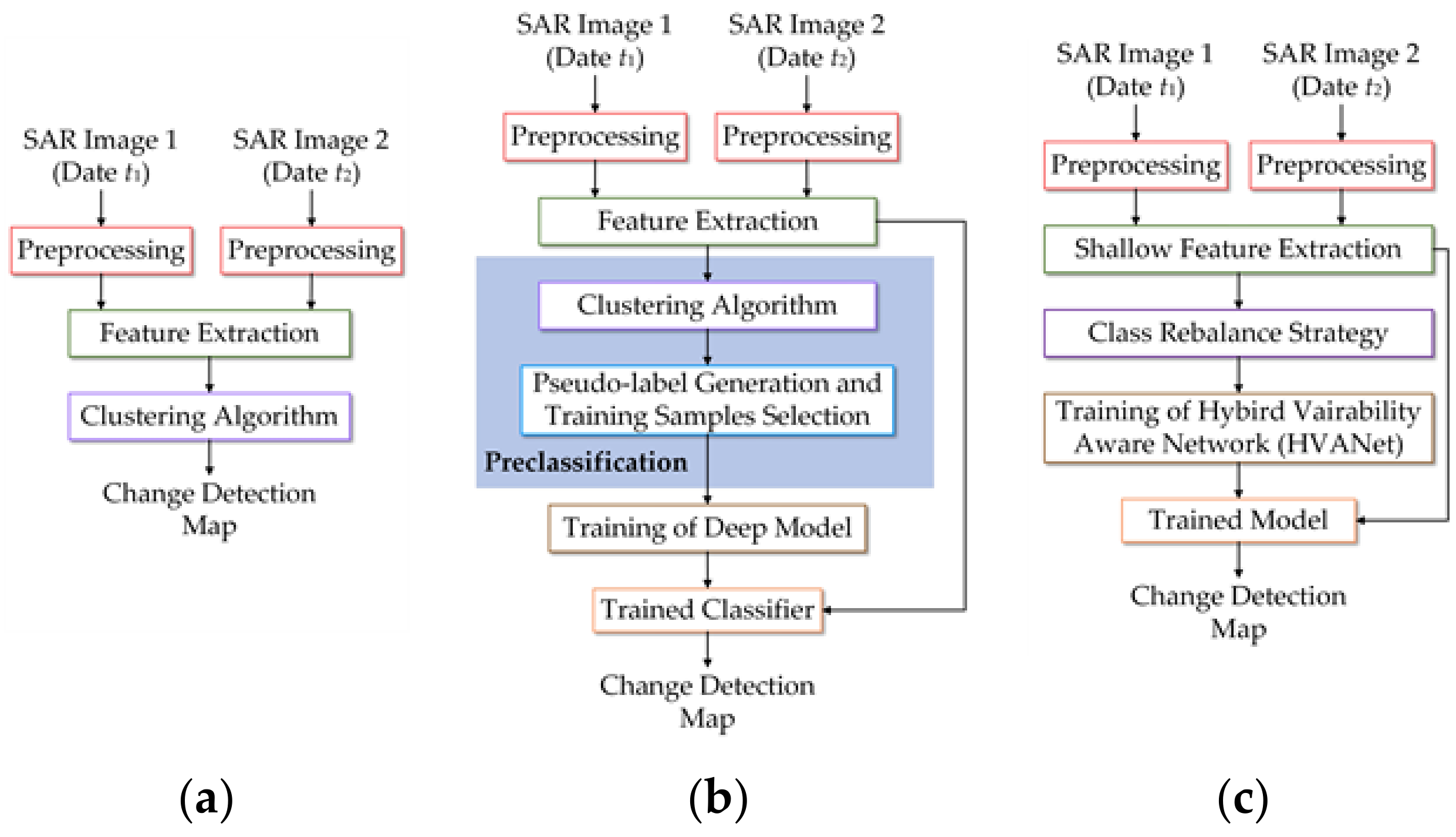
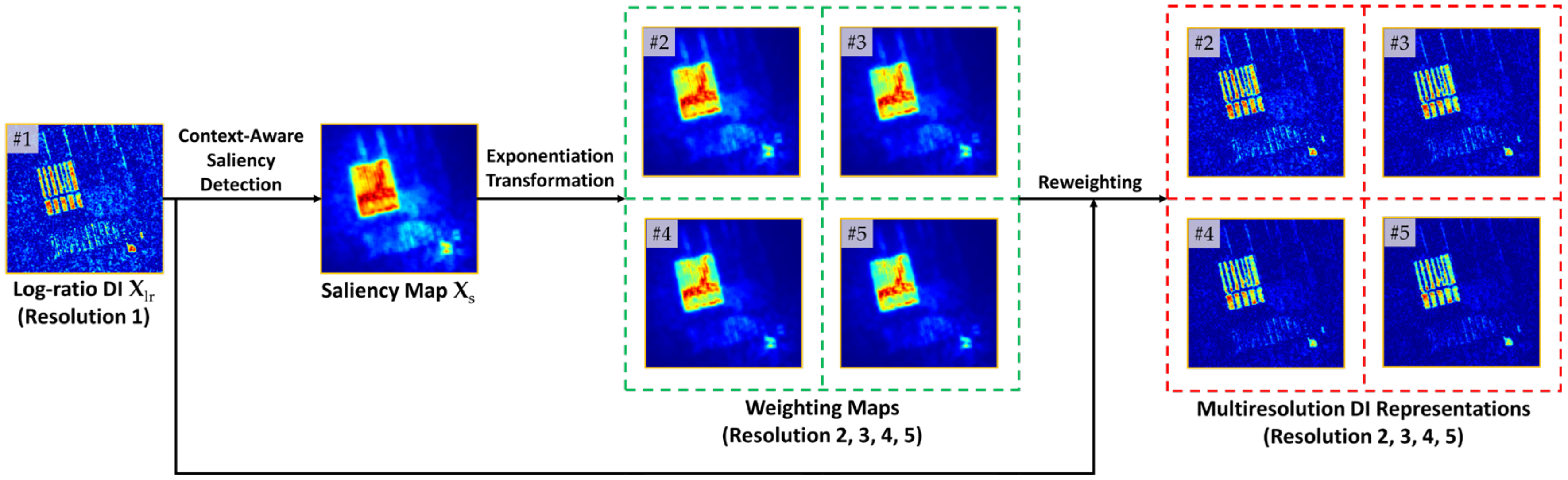
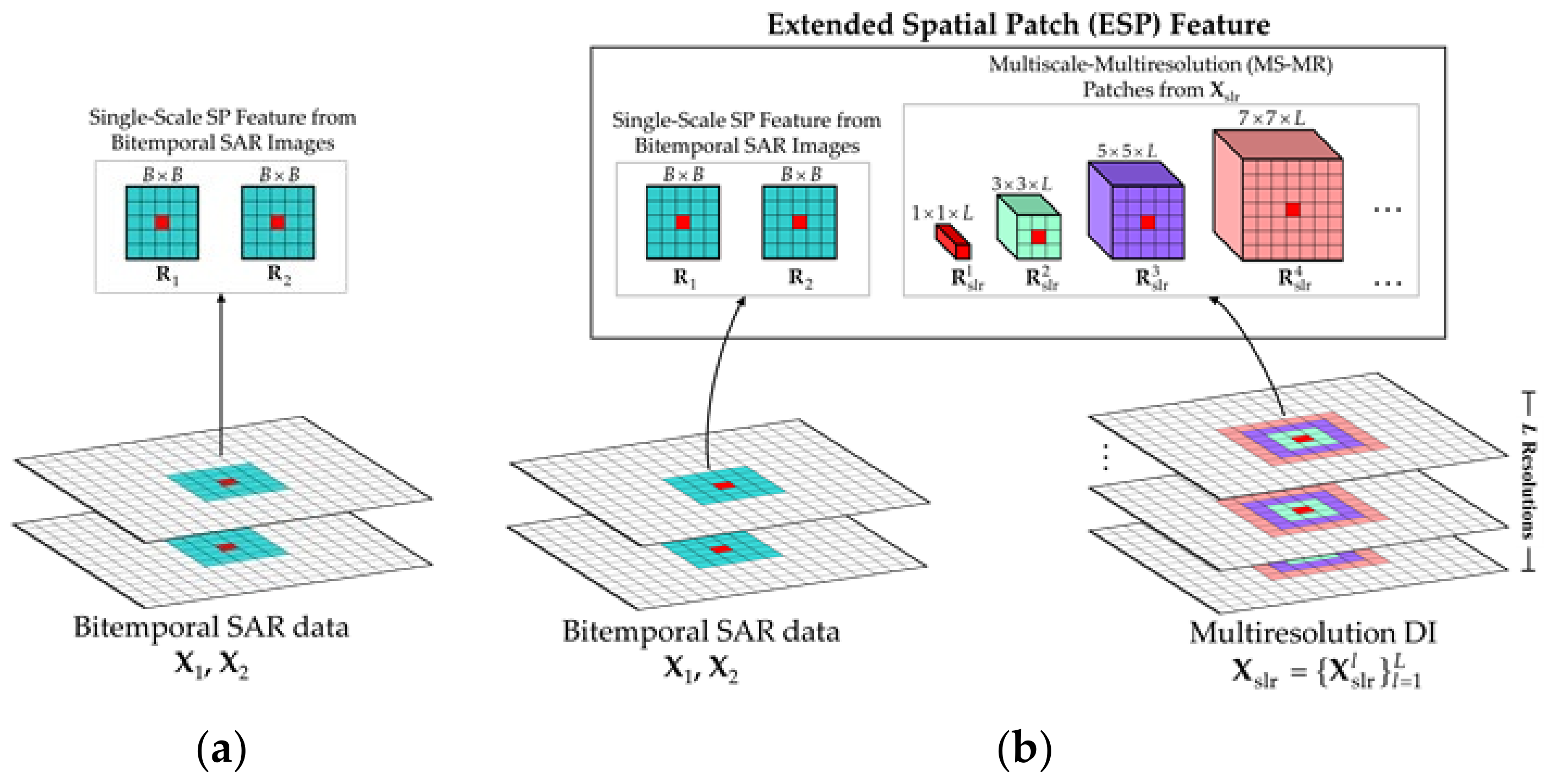
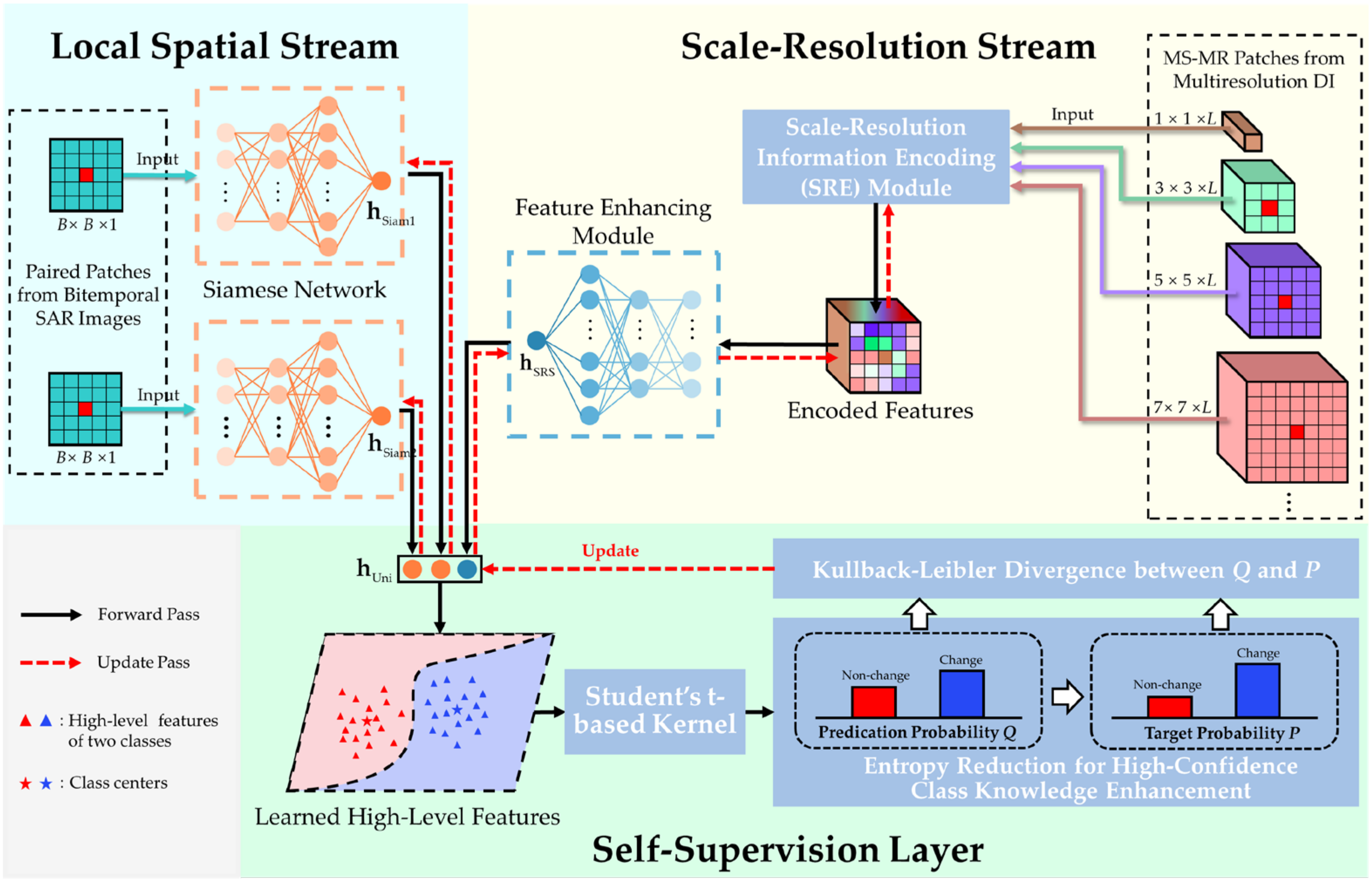
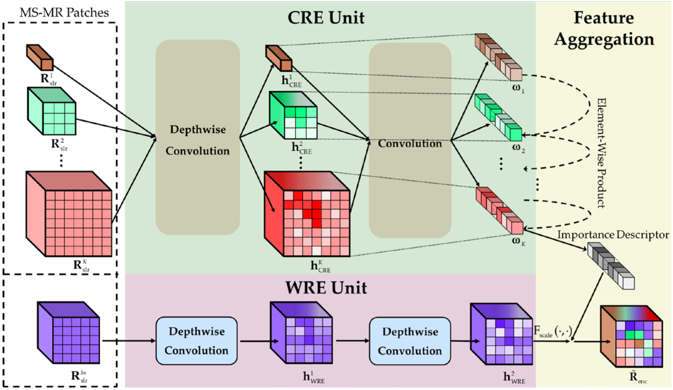
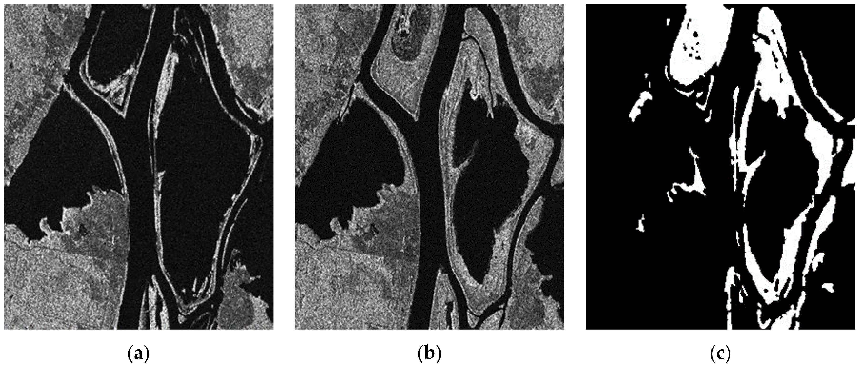
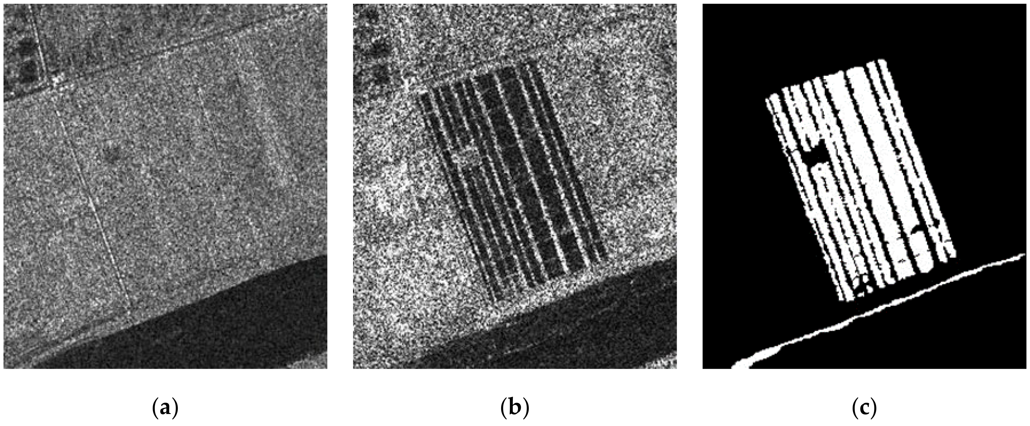
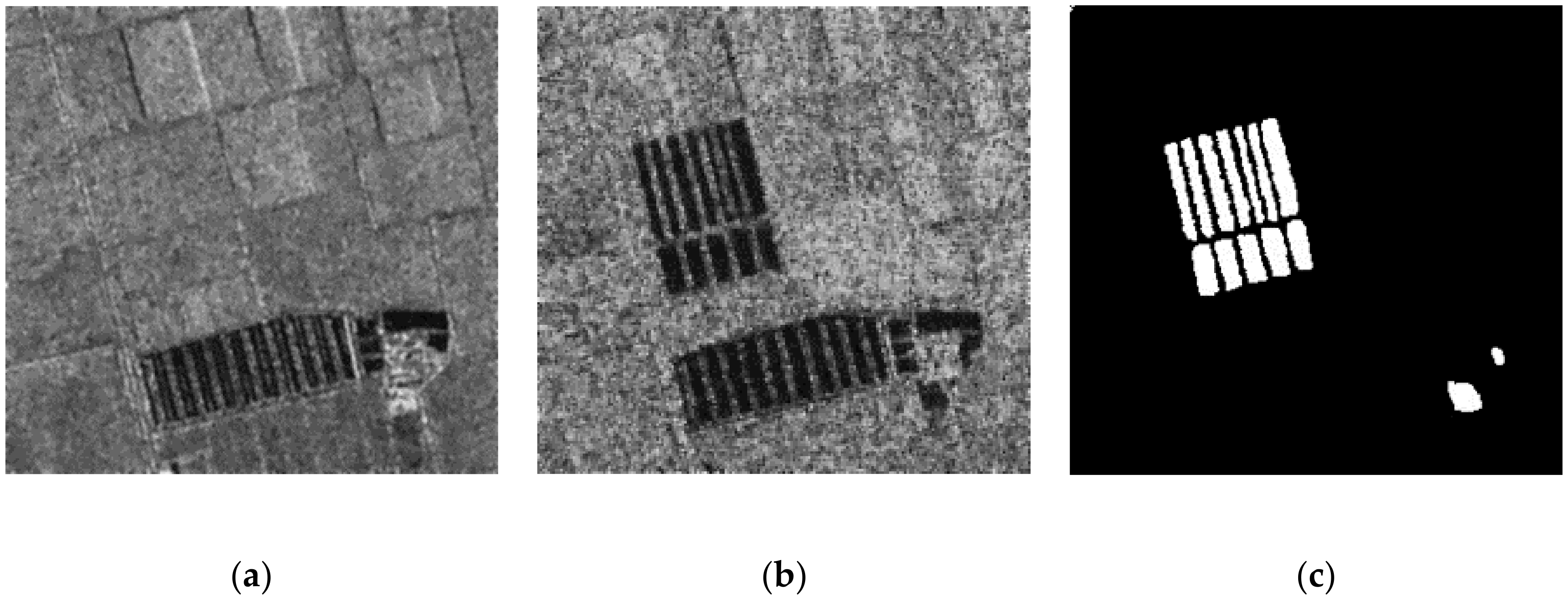
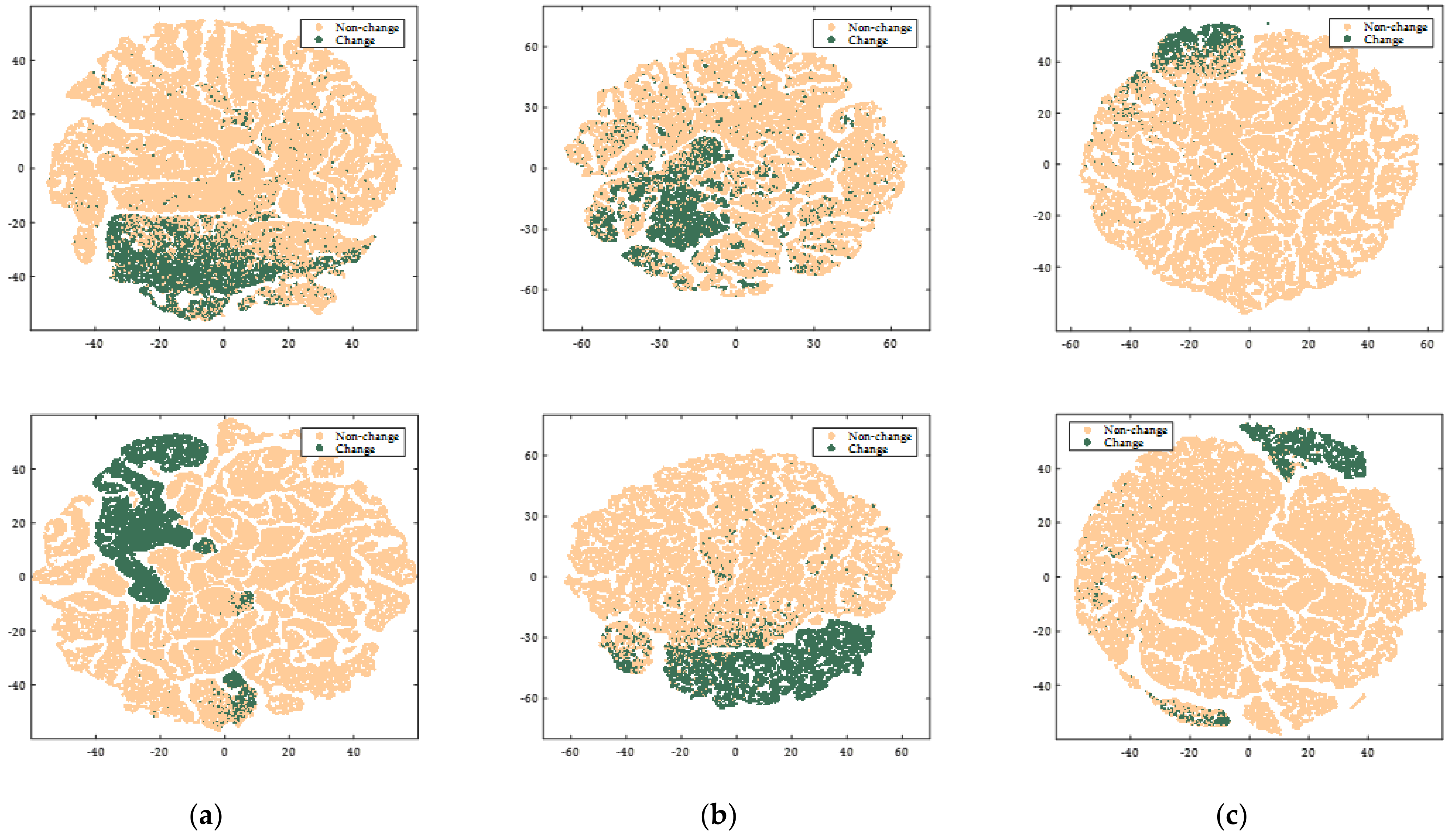
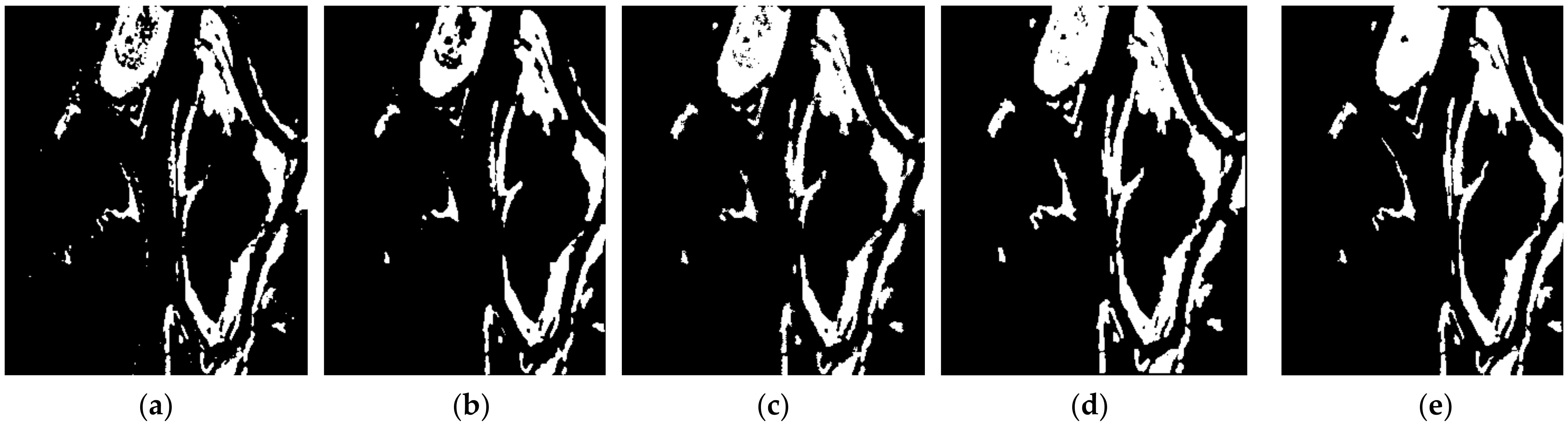
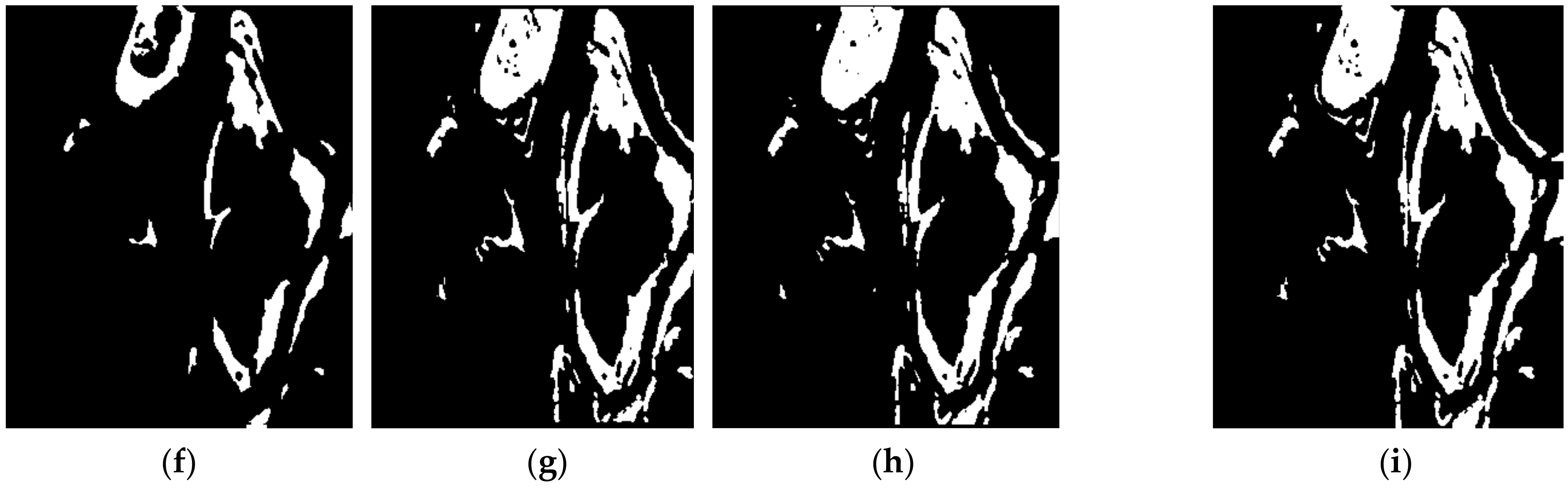
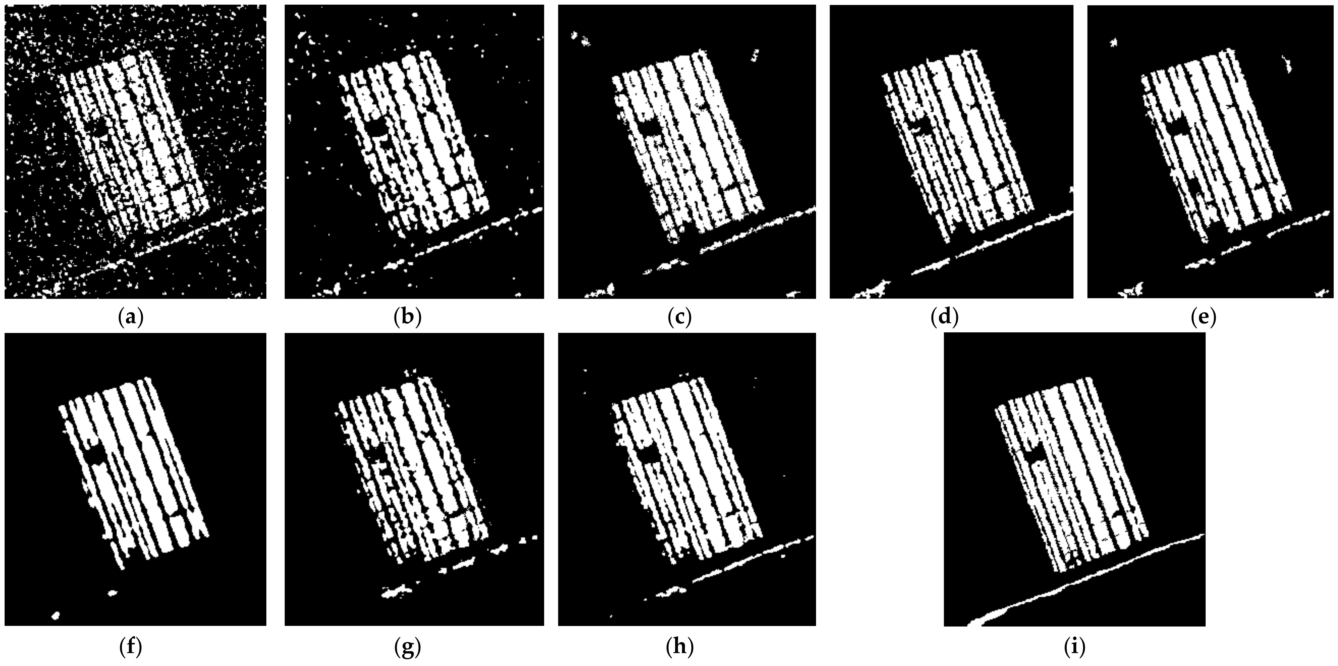
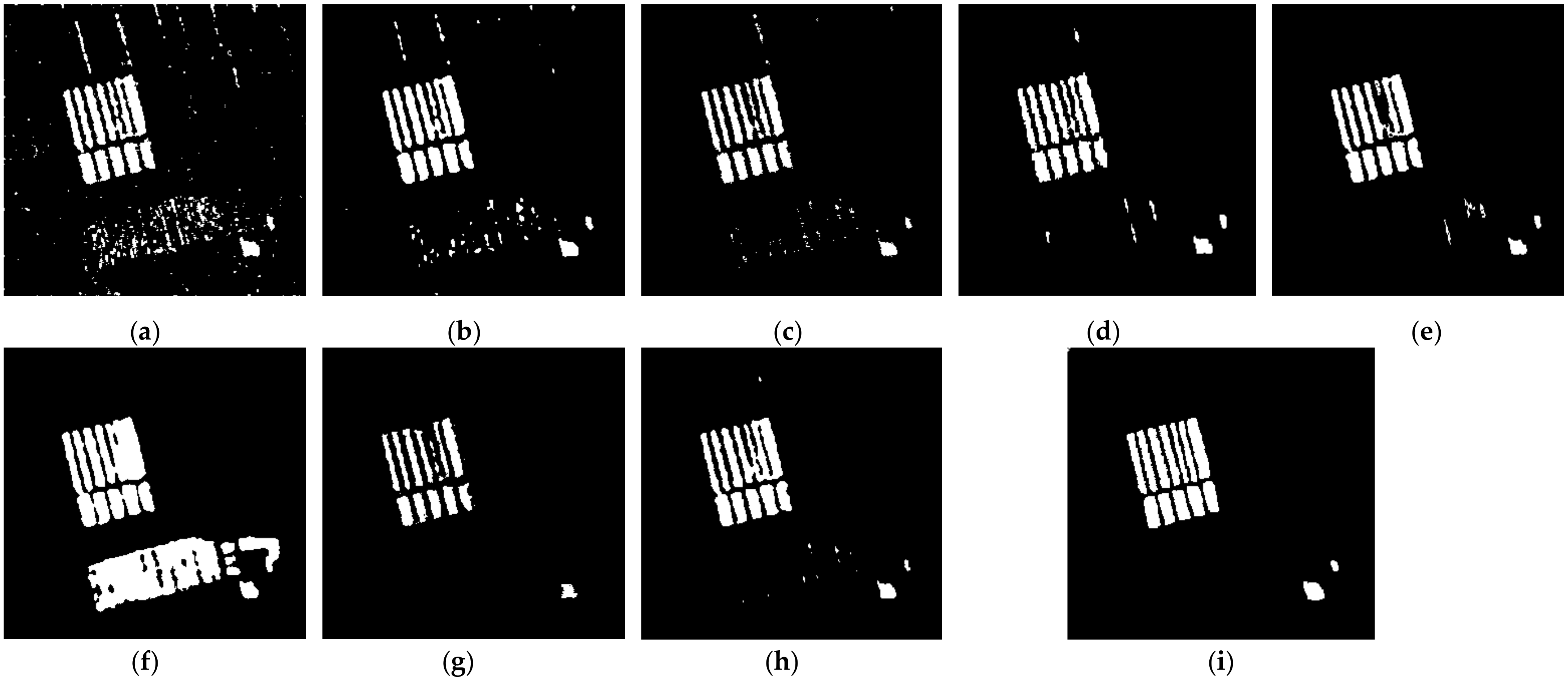
Table 1.
Architecture of the proposed HVANet.
| HVANet Configuration | |
|---|---|
| Local Spatial Stream | |
| Fully Connected Layers | (B × B) × 750 × 750 × 1500 × 1 |
| Nonlinearity: SELU | |
| Scale-Resolution Stream | |
| SRE Module | |
| at basic scale | Depthwise Conv 1 × 1 |
| Nonlinearity: SELU | |
| Depthwise Conv 1 × 1 | |
| Nonlinearity: SELU | |
| Depthwise Conv 1 × 1 | |
| Nonlinearity: SELU | |
| Conv L@(2k – 1) × (2k – 1) | |
| Nonlinearity: Sigmoid | |
| FE Module | |
| Fully Connected Layers | (B × B × L) × 750 × 750 × 1500 × 1 |
| Nonlinearity: SELU | |
Table 2.
Ablation study results of the proposed HVANet on SiamNet.
| Model | LSS (SiamNet) | SRS | Ottawa | Farmland A | Farmland B | ||||
|---|---|---|---|---|---|---|---|---|---|
| SRE | FE | PCC | Kappa | PCC | Kappa | PCC | Kappa | ||
| DNN | 93.96 | 80.04 | 94.67 | 82.15 | 95.44 | 68.41 | |||
| LSS (SiamNet) | √ | 93.98 | 79.99 | 95.07 | 83.18 | 95.49 | 68.33 | ||
| DNN + SRS | √ | √ | 98.22 | 93.41 | 96.12 | 86.28 | 98.83 | 89.26 | |
| HVANet (LSS +SRS) | √ | √ | √ | 98.59 | 94.64 | 96.29 | 87.12 | 98.99 | 90.70 |
Table 3.
Ablation study results of the proposed HVANet on SRS.
| Model | LSS | SRS | Ottawa | Farmland A | Farmland B | ||||
|---|---|---|---|---|---|---|---|---|---|
| (SiamNet) | SRE | FE | PCC | Kappa | PCC | Kappa | PCC | Kappa | |
| LSS (SiamNet) | √ | 93.98 | 79.99 | 95.07 | 83.18 | 95.49 | 68.33 | ||
| HVANet | √ | √ | 97.23 | 90.02 | 96.12 | 86.48 | 98.95 | 90.61 | |
| HVANet | √ | √ | √ | 98.59 | 94.64 | 96.29 | 87.12 | 98.99 | 90.70 |
| DNN | 93.96 | 80.04 | 94.67 | 82.15 | 95.44 | 68.41 | |||
| DNN + SRS | √ | √ | 98.22 | 93.41 | 96.12 | 86.28 | 98.83 | 89.26 | |
Table 4.
Ablation study results of the proposed HVANet on class rebalance strategy.
| Model | Sample Strategy | Ottawa | Farmland A | Farmland B | ||||
|---|---|---|---|---|---|---|---|---|
| K-Means | Class | PCC | Kappa | PCC | Kappa | PCC | Kappa | |
| Clustering | Rebalance | |||||||
| HVANet | √ | 98.38 | 93.95 | 95.81 | 84.98 | 98.90 | 89.65 | |
| HVANet | √ | 98.59 | 94.64 | 96.29 | 87.12 | 98.99 | 90.70 | |
Table 5.
Effect of the scale number.
| Scale Number | Scale Setting | Ottawa | Farmland A | Farmland B | |||
|---|---|---|---|---|---|---|---|
| PCC | Kappa | PCC | Kappa | PCC | Kappa | ||
| K = 1 | 1 | 98.12 | 92.93 | 95.08 | 81.82 | 98.47 | 85.89 |
| K = 2 | 1, 3 | 98.30 | 93.59 | 95.15 | 82.67 | 98.56 | 86.42 |
| K = 3 | 1, 3, 5 | 98.59 | 94.64 | 96.29 | 87.12 | 98.99 | 90.70 |
| K = 4 | 1, 3, 5, 7 | 98.21 | 93.22 | 95.22 | 82.72 | 98.77 | 88.36 |
| K = 5 | 1, 3, 5, 7, 9 | 98.00 | 92.53 | 95.39 | 85.43 | 99.09 | 91.60 |
Table 6.
Sensitivity analysis of the HVANet in relation to patch size.
| Basic Scale | Ottawa | Farmland A | Farmland B | |||
|---|---|---|---|---|---|---|
| PCC | Kappa | PCC | Kappa | PCC | Kappa | |
| 3 × 3 | 98.59 | 94.64 | 95.94 | 85.83 | 98.85 | 89.19 |
| 5 × 5 | 98.34 | 93.65 | 96.29 | 87.12 | 98.99 | 90.70 |
| 7 × 7 | 98.17 | 93.03 | 95.71 | 84.73 | 98.72 | 89.81 |
| 9 × 9 | 97.89 | 92.17 | 95.25 | 82.96 | 98.49 | 86.02 |
Table 7.
Effect of the resolution number.
| Resolution Number | Ottawa | Farmland A | Farmland B | |||
|---|---|---|---|---|---|---|
| PCC | Kappa | PCC | Kappa | PCC | Kappa | |
| 1 | 98.14 | 92.85 | 95.66 | 84.39 | 98.58 | 87.06 |
| 2 | 98.36 | 93.91 | 95.92 | 86.35 | 98.73 | 87.95 |
| 3 | 98.51 | 94.29 | 96.17 | 86.58 | 98.83 | 89.29 |
| 4 | 98.48 | 94.06 | 96.25 | 86.91 | 98.97 | 90.39 |
| 5 | 98.59 | 94.64 | 96.29 | 87.12 | 98.99 | 90.70 |
Table 8.
Change detection results of each method on Ottawa dataset.
| Method | FP | FN | OE | PCC | Kappa |
|---|---|---|---|---|---|
| PCA-kmeans | 589 | 1898 | 2487 | 97.55 | 90.49 |
| GaborTLC | 1249 | 497 | 1746 | 98.28 | 87.63 |
| PCANet | 995 | 853 | 1848 | 98.18 | 93.22 |
| DDNet | 622 | 1186 | 1808 | 98.22 | 93.21 |
| CWNN | 1291 | 434 | 1725 | 98.30 | 93.75 |
| INLPG-CWNN | 0 | 7039 | 7039 | 93.07 | 68.31 |
| SGDNNs | 0 | 1067 | 1067 | 98.95 | 95.94 |
| HVANet | 497 | 934 | 1431 | 98.59 | 94.64 |
Table 9.
Change detection results of each method on Farmland A dataset.
| Method | FP | FN | OE | PCC | Kappa |
|---|---|---|---|---|---|
| PCA-kmeans | 4211 | 3365 | 7576 | 89.80 | 66.40 |
| GaborTLC | 1656 | 2867 | 4523 | 93.91 | 78.69 |
| PCANet | 1716 | 1686 | 3402 | 95.42 | 84.55 |
| DDNet | 952 | 1846 | 2798 | 96.23 | 86.95 |
| CWNN | 837 | 1690 | 2527 | 96.60 | 88.23 |
| INLPG-CWNN | 510 | 2409 | 2919 | 96.07 | 85.96 |
| SGDNNs | 862 | 2894 | 3756 | 94.94 | 81.86 |
| HVANet | 891 | 1864 | 2755 | 96.29 | 87.12 |
Table 10.
Change detection results of each method on the Farmland B dataset.
| Method | FP | FN | OE | PCC | Kappa |
|---|---|---|---|---|---|
| PCA-kmeans | 2235 | 623 | 2858 | 96.79 | 74.78 |
| GaborTLC | 748 | 703 | 1451 | 98.37 | 85.44 |
| PCANet | 356 | 1265 | 1621 | 98.54 | 85.40 |
| DDNet | 155 | 1211 | 1366 | 98.47 | 84.80 |
| CWNN | 225 | 863 | 1088 | 98.78 | 88.37 |
| INLPG-CWNN | 7007 | 22 | 7029 | 91.88 | 54.53 |
| SGDNNs | 18 | 1848 | 1866 | 97.90 | 77.53 |
| HVANet | 302 | 597 | 899 | 98.99 | 90.70 |
Table 11.
The average evaluation criteria of different methods for the three datasets.
| Method | FP | FN | OE | PCC | Kappa |
|---|---|---|---|---|---|
| PCA-kmeans | 2345 | 1962 | 4307 | 94.71 | 77.22 |
| GaborTLC | 1217 | 1356 | 2573 | 96.85 | 83.92 |
| PCANet | 1022 | 1268 | 2290 | 97.38 | 87.72 |
| DDNet | 577 | 1414 | 1991 | 97.64 | 88.32 |
| CWNN | 784 | 996 | 1780 | 97.89 | 90.12 |
| INLPG-CWNN | 2505 | 3157 | 5662 | 93.67 | 69.60 |
| SGDNNs | 294 | 1936 | 2230 | 97.26 | 85.11 |
| HVANet | 563 | 1132 | 1695 | 97.96 | 90.82 |
Table 12.
Computational costs of different SAR image CD methods (in seconds).
| Method | Ottawa Dataset | Farmland A Dataset | Farmland B Dataset | |||
|---|---|---|---|---|---|---|
| Training Time | Inference Time | Training Time | Inference Time | Training Time | Inference Time | |
| PCA-kmeans | - | 1.34 | - | 2.51 | - | 1.37 |
| GaborTLC | - | 3.29 | - | 4.37 | - | 4.18 |
| PCANet | 621.92 | 300.65 | 501.93 | 541.17 | 555.48 | 303.72 |
| DDNet | 596.85 | 17.69 | 618.41 | 18.54 | 454.89 | 17.21 |
| CWNN | 547.23 | 15.81 | 549.37 | 15.62 | 543.56 | 12.49 |
| HVANet | 327.76 | 9.41 | 710.74 | 12.28 | 565.23 | 16.45 |
Publisher’s Note: MDPI stays neutral with regard to jurisdictional claims in published maps and institutional affiliations. |
© 2022 by the authors. Licensee MDPI, Basel, Switzerland. This article is an open access article distributed under the terms and conditions of the Creative Commons Attribution (CC BY) license (https://creativecommons.org/licenses/by/4.0/).
Share and Cite
MDPI and ACS Style
Wang, J.; Wang, Y.; Liu, H. Hybrid Variability Aware Network (HVANet): A Self-Supervised Deep Framework for Label-Free SAR Image Change Detection. Remote Sens. 2022, 14, 734. https://0-doi-org.brum.beds.ac.uk/10.3390/rs14030734
AMA Style
Wang J, Wang Y, Liu H. Hybrid Variability Aware Network (HVANet): A Self-Supervised Deep Framework for Label-Free SAR Image Change Detection. Remote Sensing. 2022; 14(3):734. https://0-doi-org.brum.beds.ac.uk/10.3390/rs14030734
Chicago/Turabian StyleWang, Jian, Yinghua Wang, and Hongwei Liu. 2022. "Hybrid Variability Aware Network (HVANet): A Self-Supervised Deep Framework for Label-Free SAR Image Change Detection" Remote Sensing 14, no. 3: 734. https://0-doi-org.brum.beds.ac.uk/10.3390/rs14030734
Note that from the first issue of 2016, this journal uses article numbers instead of page numbers. See further details here.