
Video Satellite Imagery Super-Resolution via Model-Based Deep Neural Networks


1
Southern Marine Science and Engineering Guangdong Laboratory (Zhuhai), School of Geography and Planning, Sun Yat-sen University, Guangzhou 510275, China
2
National Key Laboratory of Science and Technology on Automatic Target Recognition, Changsha 410073, China
3
Department of Mathematics, Harbin Institute of Technology, Weihai 264209, China
*
Author to whom correspondence should be addressed.
Remote Sens. 2022, 14(3), 749; https://0-doi-org.brum.beds.ac.uk/10.3390/rs14030749
Submission received: 12 November 2021
/
Revised: 19 December 2021
/
Accepted: 19 January 2022
/
Published: 6 February 2022
Abstract
:Video satellite imagery has become a hot research topic in Earth observation due to its ability to capture dynamic information. However, its high temporal resolution comes at the expense of spatial resolution. In recent years, deep learning (DL) based super-resolution (SR) methods have played an essential role to improve the spatial resolution of video satellite images. Instead of fully considering the degradation process, most existing DL-based methods attempt to learn the relationship between low-resolution (LR) satellite video frames and their corresponding high-resolution (HR) ones. In this paper, we propose model-based deep neural networks for video satellite imagery SR (VSSR). The VSSR is composed of three main modules: degradation estimation module, intermediate image generation module, and multi-frame feature fusion module. First, the blur kernel and noise level of LR video frames are flexibly estimated by the degradation estimation module. Second, an intermediate image generation module is proposed to iteratively solve two optimal subproblems and the outputs of this module are intermediate SR frames. Third, a three-dimensional (3D) feature fusion subnetwork is leveraged to fuse the features from multiple video frames. Different from previous video satellite SR methods, the proposed VSSR is a multi-frame-based method that can merge the advantages of both learning-based and model-based methods. Experiments on real-world Jilin-1 and OVS-1 video satellite images have been conducted and the SR results demonstrate that the proposed VSSR achieves superior visual effects and quantitative performance compared with the state-of-the-art methods.
1. Introduction
Over the past few years, video satellite imagery [1,2,3,4] has received considerable attention in the remote sensing and aerospace field. Compared with the traditional satellites that obtain static images [5,6,7,8], video satellite provides a novel way to capture continuous videos. It can acquire dynamic information from the objects on the Earth’s surface and thus has great advantages in dynamic monitoring, such as moving ship detection [9], object tracking [10], and object detection [11]. However, for the sake of increased temporal resolution and the degradation in imaging procedures, the spatial resolution is lost to a certain extent, which hinders the further application of video satellites. Super-resolution (SR) [12,13,14] is an effective way to recover the sharp and natural high-resolution (HR) images (or sequence) from their low-resolution (LR) counterparts. Note that SR is a classical ill-posed inverse problem [15] that can increase the spatial resolution and clarity of low-quality images, it is an important but challenging task in video satellite imagery.
In the literature, much work has been devoted to improving the quality of images/videos by SR. From the perspective of the length of LR images used, SR can be categorized into single image SR (SISR) [16,17,18] and multi-image SR (MISR) [19,20,21]. SISR reconstructs the HR result by employing only a single LR version, while multiple LR images from the same scene are adopted to construct an HR image in the MISR. It is noteworthy that MISR is especially suitable for SR of video satellite images since there are amounts of continuous frames of a certain scene in one satellite video.
According to the characteristics of the technology itself, there roughly exist two common categories, i.e., model-based methods and learning-based methods. The model-based methods usually construct a degradation model under the Bayesian framework, in which the blur, downsampling, and noise processes are considered and Maximum a posteriori (MAP) [22,23,24] is utilized to estimate the HR results. The classical interpolation-based methods [25,26] can be viewed as a special model-based method, in which a predetermined interpolation pattern (e.g., bilinear or bicubic interpolation) is adopted in the degradation process. Moreover, plenty of priors and regularization terms have been proposed to improve the SR performance. Widespread priors or regularization terms include gradient prior [27], Markov random field (MRF) regularization [28], total variation (TV) [29] and bilateral TV regularization [30]. Model-based methods have clear physical meaning and thus algorithmically interpretable. However, the performance of this category is limited by hand-crafted priors.
The other category is learning-based methods, which aim to learn a mapping function from the training samples composed of LR and HR pairs. LR images can be obtained by downsampling the HR images. One of the basic assumptions is that the LR and HR pairs share a similar manifold structure. Typical learning-based method include the sparse representation with over-complete dictionary [31,32,33]. Sparse representation aims to represent signals/images with few significant coefficients, and sparse representation-based SR methods attempt to represent the image patches as a sparse linear combination of elements from a learned over-complete dictionary. With the rise of artificial intelligence (AI), deep learning (DL)-based methods have dominated SR research in recent years. Among all the DL-based methods, the convolutional neural network (CNN) is the most popular owing to its powerful ability to express abstract features. For instance, the SR method via a CNN (SRCNN) [34] with three layers proposed by Dong et al. has opened a new era. A very deep convolutional network for accurate image super-resolution (VDSR) [35], which increases the network depth to 20 layers, is proposed by Kim et al. Afterward, Lim et al. [36] develop an enhanced deep super-resolution network (EDSR) to significantly improve the SR performance by removing unnecessary modules and expanding the model size. Notably that the feed-forward structure cannot fully address the mutual dependencies between LR and HR pairs, Haris et al. [37] propose deep back-projection networks (DBPN) to provide error feedback mechanism at multiple upsampling and downsampling stages. After that, a second-order attention network (SAN) [38] is proposed by Dai et al. to explore the feature correlations among intermediate layers instead of designing wider or deeper architectures.
In recent years, researchers have also devoted themselves to the SR of video satellite images. Inspired by VDSR, Luo et al. [39] design a rectified CNN to reconstruct HR video satellite images. Xiao et al. [40] propose a deep CNN-based method without using any pre-processing and post-processing, while Jiang et al. [41] develop a progressively enhanced CNN (PECNN) for satellite imagery SR by using dense connections and progressive feature learning. Deep distillation recursive network (DDRN) [42] and generative adversarial network (GAN)-based edge-enhancement network (EEGAN) [43] are also successively proposed by Jiang et al. Although the above-mentioned DL-based methods have proven to perform well, there still exist some drawbacks. These methods generally focus on establishing the connection of LR-HR data and fail to fully characterize the degradation process, which is detrimental for model generalization and physical interpretability, hindering the further improvement of the SR effect. Recently, some researchers have realized this problem and attempt to combine the learning-based methods with model-based ones. For instance, Pan et al. [44] propose a deep blind video SR (DBVSR) method, in which the blur kernel is estimated by two fully connected layers. However, the noise level is ignored. Moreover, Zhang et al. [45] propose an unfolding SR network (USRNet) under the MAP inference by a half-quadratic splitting strategy. However, USRNet is a SISR method, which cannot fully use the spatial-temporal information of adjacent frames. In addition, both the blur kernel and noise level in the USRNet should be preset in advance.
To overcome the above-mentioned drawbacks, we propose a video satellite imagery SR method termed VSSR. The proposed VSSR is composed of three main modules, i.e., degradation estimation module, intermediate image generation module, and multi-frame feature fusion module. The degradation estimation module is designed to estimate the blur kernel and noise level of the input LR frames. The intermediate image generation module is utilized to unfold the MAP framework and iteratively solve two optimal subproblems, while the multi-frame feature fusion module is constructed to fuse the features from multiple adjacent video frames. To sum up, the main innovative contributions of this work lie in the following three aspects:
- We propose a novel VSSR method for video satellite imagery SR. To the best of our knowledge, it is the first attempt to combine DL and model-based methods in the field of video satellite SR.
- The proposed VSSR can split the SR problem into two sub-optimization problems under the umbrella of the MAP framework. One of the subproblems has an analytical solution, and the other subproblem is solved by subnetworks. By alternatively optimizing the sub-optimization problems, we can obtain intermediate SR results.
- The proposed VSSR can leverage the information from adjacent frames through a three-dimensional (3D) feature fusion subnetwork. Different from the SISR methods or the MISR methods based on optical flow estimation, the VSSR is a MISR method, in which the features from multiple frames are effectively fused by 3D residual blocks.
The remainder of this paper is organized as follows. In Section 1, the proposed VSSR is described in detail. In Section 2.2.5, the experimental results and analysis are reported. Finally, this paper is concluded in Section 5.
2. Materials and Methods
2.1. Data Collection
In this paper, we collect the real-world Jilin-1 and OVS-1 video satellite data (see Table 1) as materials. A detailed description of those two datasets is given as follows:
- Jilin-1 data: the first video satellite dataset was acquired by the Chinese Jilin-1 satellite of Chang Guang Satellite Technology Co., Ltd., Changchun, China (http://charmingglobe.com/, accessed on 10 September 2021) This dataset contains 13 videos from various countries covering buildings, airports, roads, flyovers, ports, forests, and so on. As displayed in Table 1, the duration of each video varies from 9 to 30 s. 10 frames with 1280 × 1280 spatial pixels and 3 RGB bands from each video is extracted for experiments. The spatial resolution of Jilin-1 data is about 1 m. The first 10 videos are used for training, while the last 3 videos (i.e., San-ya, San Diego, and Macao) are for testing.
- OVS-1 data: the second video satellite dataset was collected by the Chinese OVS-1 satellite of Zhuhai Orbita Aerospace Science & Technology Co., Ltd., Zhuhai, China, (https://www.myorbita.net/index.aspx, accessed on 10 September 2021). This dataset consists of 2 videos (i.e., Dalian and Marseille) covering city and port regions. The duration time of the videos is 29 and 34 s, respectively. We extract 10 frames from those 2 videos and all frames are cropped to 600 × 600 spatial pixels with 3 RGB bands. The spatial resolution of OVS-1 data is 1.98 m. Both videos are used for testing by feeding the downsampled video frames into trained networks.
2.2. Proposed Method
In this section, we explain the proposed VSSR method in detail, including the network architecture (see Figure 1) and the loss function for model optimization.
2.2.1. Network Architecture of the VSSR
The overall architecture of the proposed VSSR method is shown in Figure 1, which inputs consecutive LR frames from the video satellite, and outputs the SR result of the center frame . For simplicity, we show the scenario with in Figure 1. To fully analyze the degradation process, we formulate the degradation model of LR and HR pairs as
where and denote the LR and HR images, respectively, represents the blur kernel, denotes downsampling, and is the additive Gaussian noise with noise level .
Equation (1) has been extensively discussed in the model-based SR methods, in which the optimization objective function can be expressed as the following combination of a data term and a prior term under the MAP framework
where is the data term, refers to the prior term, and denotes the trade-off between the data term and prior term.
By adopting the half-quadratic splitting algorithm, we introduce an auxiliary variable and rewrite Equation (2) as
where is the penalty parameter.
Therefore, the problem in Equation (3) can be split into the following two subproblems
where Equations (4) and (5) are associated with and respectively, and and are the solution in the j-th iteration.
Apparently, Equation (4) has analytical solution since it is a least square problem, whose solution can be modeled as
where the matrix , denotes the conjugate transpose, s is the scale factor, refers to the Fourier transform, , in which the matrix satisfies the relationship , the diagonal elements of the diagonal matrix are the Fourier coefficients of the first column of the blur kernel , and denotes the identity matrix.
For Equation (5), it is actually a denoising problem with noise level . Motivated by [46,47], we propose a wavelet-based U-net to estimate the clear .
In VSSR, each LR frame from can be represented by Equation (1) and the corresponding HR frame can be obtained by iteratively solving Equations (4) and (5). Subsequently, all the estimated adjacent HR frames are stacked and fed into a 3D feature fusion subnetwork, which can effectively use the features from multiple frames. In a nutshell, the VSSR is composed of three main modules, i.e., degradation estimation module, intermediate image generation module, and multi-frame feature fusion module (see Figure 1), whose details are as follows.
2.2.2. Degradation Estimation Module
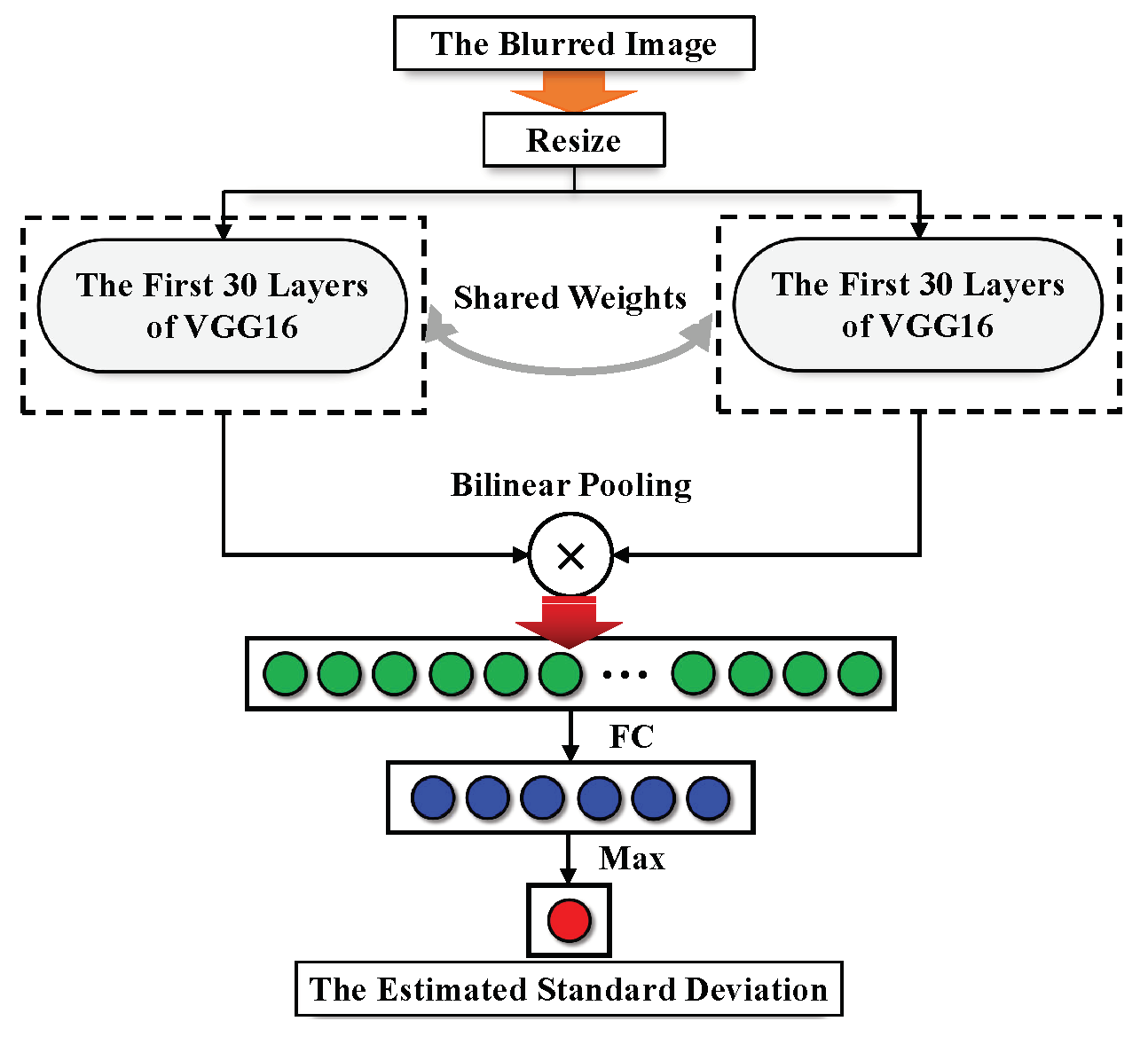
In the degradation estimation module, the noise level estimation and blur kernel estimation are respectively performed on the input LR frames. As to the noise level estimation, we calculate the noise level of the center frame by referring [48]. As to the blur kernel estimation, we assume the LR frames suffer from Gaussian blur and design a fine-grained classification-based subnetwork to estimate the standard deviation of the blur kernel. In greater detail, the standard deviation is divided into 6 classes, i.e., , each category is quite similar, and therefore, the fine-grained classification method is suitable for recognizing the classes with small inter-category variations [49]. As illustrated in Figure 2, the blur kernel estimation subnetwork accepts the blurred image as input and outputs the estimated standard deviation
where is the blur kernel estimation subnetwork, is the standard deviation, denotes the blurred image, represents a set of parameters in . It is shown from Figure 2 that the embedded features are extracted by the first 30 layers of VGG16 [50] and bilinear pooling is adopted to combine the pairwise interactions between features extracted by the two subnetworks with shared weights. To optimize the parameters , The following two loss terms are utilized
where
here and are the cross entropy loss and loss, respectively, is a trade-off parameter, is the output vector of the fully connected layer (FC) in , refers to the ground truth class of the standard deviation, is the ground truth blur kernel, and denotes the estimated kernel.
2.2.3. Intermediate Image Generation Module
In the intermediate image generation module, the auxiliary variable and HR image are iteratively solved. The closed-form solution of is calculated by Equation (6), while is estimate by the wavelet-based U-net. In greater detail, it is observed from Figure 1 that the calculation block takes , s, and as input and outputs . Moreover, we design a (see Figure 3 and Figure 4), which utilizes and to estimate . Specifically, can be formulated as
where refers to the parameters to be optimized in . Discrete wavelet transform (DWT) and inverse wavelet transform (IWT) are used as downsampling and upsampling layers in to enlarge the receptive field.
As to the parameters, the standard deviation of is obtained by , s represents the scale factor, and the parameters and are generated by the hyper-parameter estimation subnetwork, which is simply composed of three fully connected layers with two rectified linear units (ReLU) [51] as the former two activation functions and Softplus [52] as the last.
2.2.4. Multi-Frame Feature Fusion Module
In the multi-frame feature fusion module, all the estimated intermediate HR frames of the input LR frames are stacked and put into a 3D feature fusion subnetwork (see Figure 5), which utilizes several 3D residual blocks to fuse the information of adjacent frames. The final SR result of the central frame is generated by , which can be modeled as
where are the HR results of the th frame obtained by the intermediate image generation module, denotes the parameters of , and refers to the final SR result of the proposed VSSR.
2.2.5. Model Optimization
In VSSR, we use the following loss as loss term to optimize the parameters , and the parameters in the hyper-parameter estimation subnetwork
where and denote the final SR results obtained by the VSSR and the corresponding reference result, respectively. Moreover, we adopt the widely-used adaptive moment estimation (Adam) solver [53] to minimize the loss term .
3. Results
In this section, we validate the effectiveness of our proposed VSSR by conducting a group of experiments on the real-world Jilin-1 and OVS-1 video satellite data (see Table 1). First, implementation details are introduced. Second, the VSSR is compared against state-of-the-art SR methods, and the experimental results on the Jilin-1 and OVS-1 data are displayed. Next, an ablation study is described to assess the contribution of each component. Finally, the sensitivity of different parameters is analyzed.
3.1. Implementation Details
In the experiments, we compare our VSSR method with several state-of-the-art SR methods, including bicubic interpolation (termed as Bicubic), SRCNN [34], VDSR [35], EDSR [36], DBPN [37], SAN [38], USRNet [45], DBVSR [44], and [40]. Notably, Bicubic, SRCNN, VDSR, EDSR, DBPN, SAN, USRNet, and are SISR-based methods, which directly map the single LR image into HR image, while DBVSR and VSSR are MISR-based methods, which can make use of the spatio-temporal information from neighboring LR frames. In both DBVSR and VSSR, 3 adjacent LR frames are fed into the network to reconstruct the SR result of the center frame. The Bicubic method generates the HR image by using bicubic interpolation, while the rest are DL-based methods, which learn the mapping function from LR-HR pairs. applies convolution layers and a deconvolution layer to enhance the resolution of video satellite images. USRNet, DBVSR, and VSSR perform SR by combining learning-based methods with model-based ones under the MAP framework. Besides the 10 videos from the Jilin-1 data (see Table 1), 30 additional videos download from a video website (https://pixabay.com/videos, accessed on 1 October 2021). are leveraged to enlarge the amount of training set. To maintain consistency, we also extract 10 frames with 1280 × 1280 spatial pixels and 3 RGB bands from those additional videos. By using Jilin-1 data as training samples, the learning-based methods can better understand the characteristics of satellite videos, while the 30 additional videos are conducive to increasing the quantity and diversity of the training set. Since the scale factor is more challengeable than or , we only consider in the experiments.
All the methods are performed on a workstation with Intel (R) Xeon (R) Gold 5218 [email protected] [email protected] GHz dual processor and Nvidia GeForce RTX 2080Ti GPU. For the sake of fairness, all the DL-based methods are retrained by using the same training set as VSSR. The configurations of competing methods are following their corresponding references. The detailed architectures of VSSR are illustrated in Section 2.2.1. The Equations (4) and (5) are iteratively solved by 6 times, which means the variable N in Equation (12) equals to 6. The learning rate is initialized as 0.0005, and the parameters in the Adam solver are set to 0.9 and 0.999, respectively. The patch size and batch size are set to 96 and 5, respectively, while the training is stopped within 50 epochs since more training epochs cannot lead to further significant improvement.
To quantitatively compare different SR methods, we apply 5 commonly used evaluation metrics for comparison. In greater detail, the evaluation metrics are root mean square error (RMSE), peak signal-to-noise ratio (PSNR), correlation coefficient (CC), structure similarity index (SSIM), and erreur relative globale adimensionnelle de synthèse (ERGAS). Larger PSNR, CC, and SSIM indicate better SR results, while opposite for other indicators.
3.2. Experimental Results on the Jilin-1 Data
To better understand the procedure of the VSSR, we first visualize part of the learned features in Figure 6, which displays 16 feature maps extracted by the eighth 3D residual block of (see Figure 5) for the San-ya data. Since 3D convolutions are used in , each feature map shown in Figure 6 is a RGB image. Moreover, it is observed that different structures and abstract features are learned and highlighted by different convolutional channels.
We then compare the qualitative and quantitative results of various methods in Figure 7, Figure 8 and Figure 9 and Table 2 to verify the effectiveness of the VSSR. Specifically, Figure 7, Figure 8 and Figure 9 visualize the SR results of the third frame in the San-ya, San Diego, and Macao satellite videos, respectively. The maps shown in the third and fourth rows are the enlarged counterparts of the scenes signed by red boxes in the first and second rows. In Table 2, we display evaluation results of our proposed VSSR against the competing methods on the Jilin-1 data with scale factor equals to 4. Bold and italic underline represent the best and the second-best performance, respectively. According to the experimental results on the Jilin-1 data, DL-based methods have advantages in obtaining better performance than bicubic interpolation. In most cases, Bicubic yields the lowest PSNR, CC, SSIM and the highest RMSE, and ERGAS among all SR methods. For instance, the RMSE of Bicubic is at least 0.4904 higher than DL-based methods, while the gap between Bicubic and DL-based methods is at least 0.3214 dB in PSNR. Intuitive comparisons are shown in Figure 7, Figure 8 and Figure 9, which demonstrates that Bicubic exhibits the most inaccurate and blurred image details in an aspect of visual effect. The reason for the poor results of Bicubic is that the degradation process is represented by a predefined interpolation pattern, which is not suitable for reflecting the realistic relationship between LR and its corresponding HR results in video satellite images.
As to the DL-based methods, SRCNN is inferior to other methods, EDSR leads to better results than and VDSR, DBPN has a slightly worse or comparable performance compared with EDSR. SAN yields superior performance than EDSR and DBPN, but achieves worse SR results than USRNet and DBVSR, while VSSR consistently outperforms the competing methods. For the San-ya data, the PSNR of and VDSR surpass SRCNN about 0.2075 dB and 0.5806 dB, respectively, while the PSNR of EDSR is 0.4633 and 0.0902 dB higher than and VDSR, respectively. In addition, the PSNR of DBPN is 0.0621 lower than EDSR. SAN surpasses EDSR and DBPN by 0.0683 dB and 0.1304 dB in PSNR, respectively, while the improvement of USRNet and DBVSR is at least 0.6004 dB comparing with SAN. The PSNR of VSSR is the highest among all methods. The RMSE, CC, SSIM, and ERGSA of VSSR are also better than other methods, while DBVSR achieves the second-best evaluation metrics. Similar properties can also be found in the San Diego and Macao data.
From the perspective of visual presentation, DL-based methods produce more noticeable texture details than Bicubic. As shown in Figure 7, Figure 8 and Figure 9, the SR results generated by SRCNN contain more blurred edges and artifacts than other DL-based methods. Among all the methods, the SR results of our proposed VSSR show the clearest visual effect and the sharpest edges. For instance, the outlines of domes, buildings, roads in San-ya (see Figure 7) are clearer than other methods. The streets, trees, and buildings in San Diego and Macao (see Figure 8 and Figure 9) are also closer to the ground-truth images than other methods. The aforementioned phenomena demonstrate the advantage of VSSR in reconstructing HR video satellite images.
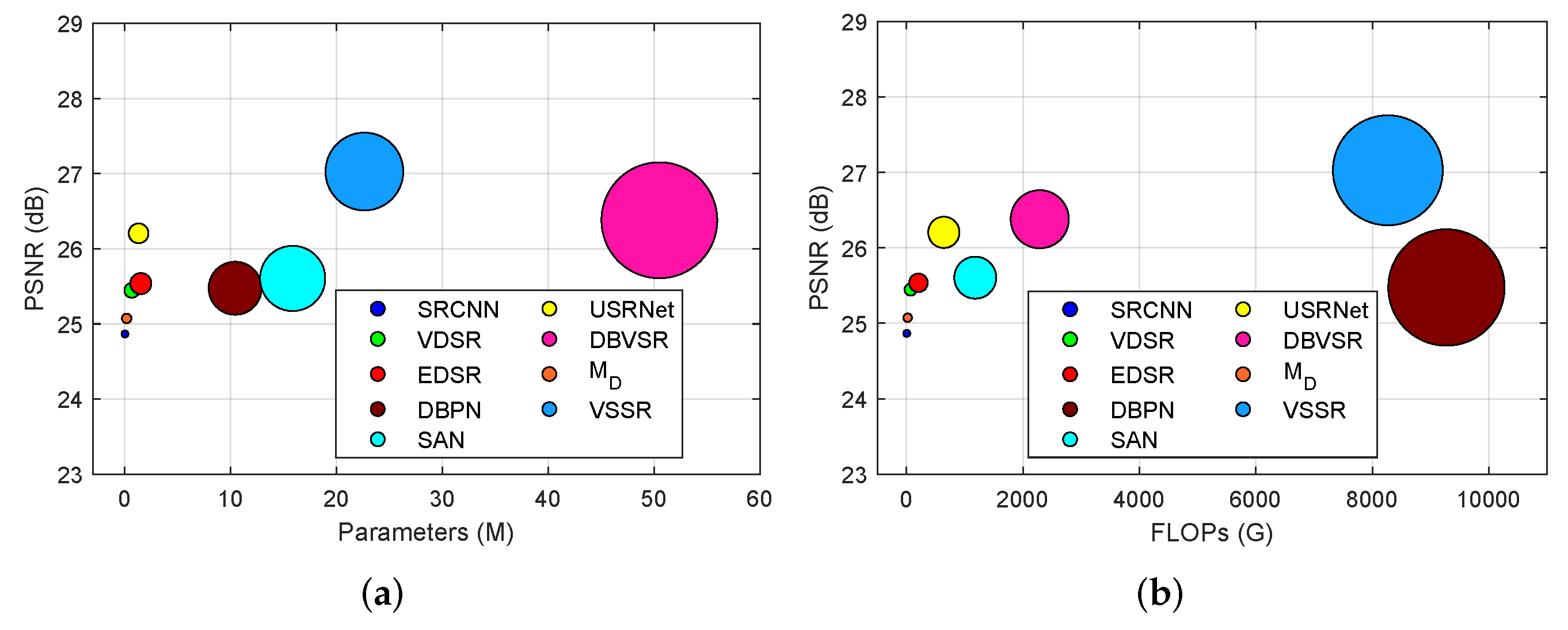
Figure 10 compares the number of parameters and floating point operations (FLOPs) of the VSSR against other DL-based approaches when we acquit a 1280 × 1280 video frame. In greater detail, Figure 10a compares the number of parameters, while Figure 10b compares the FLOPs. As shown in Figure 10a, the number of parameters of SRCNN, , VDSR, USRNet, and EDSR are relatively low, they are all less than 2 M. DBPN and SAN are within 20 M, both of which have more parameters than the five methods mentioned above. The number of parameters of VSSR is 22.6 M, and the parameter of DBVSR is 50.5 M, which is the largest among all methods. It is depicted in Figure 10b that the FLOPs of SRCNN, , and VDSR are all less than 70 G, while the FLOPs of USRNet, SAN, and DBVSR are larger than SRCNN, and VDSR. The VSSR has larger FLOPs than the other methods except DBPN, and the FLOPs of DBPN are greater than 9000 G, which is the largest among all methods.
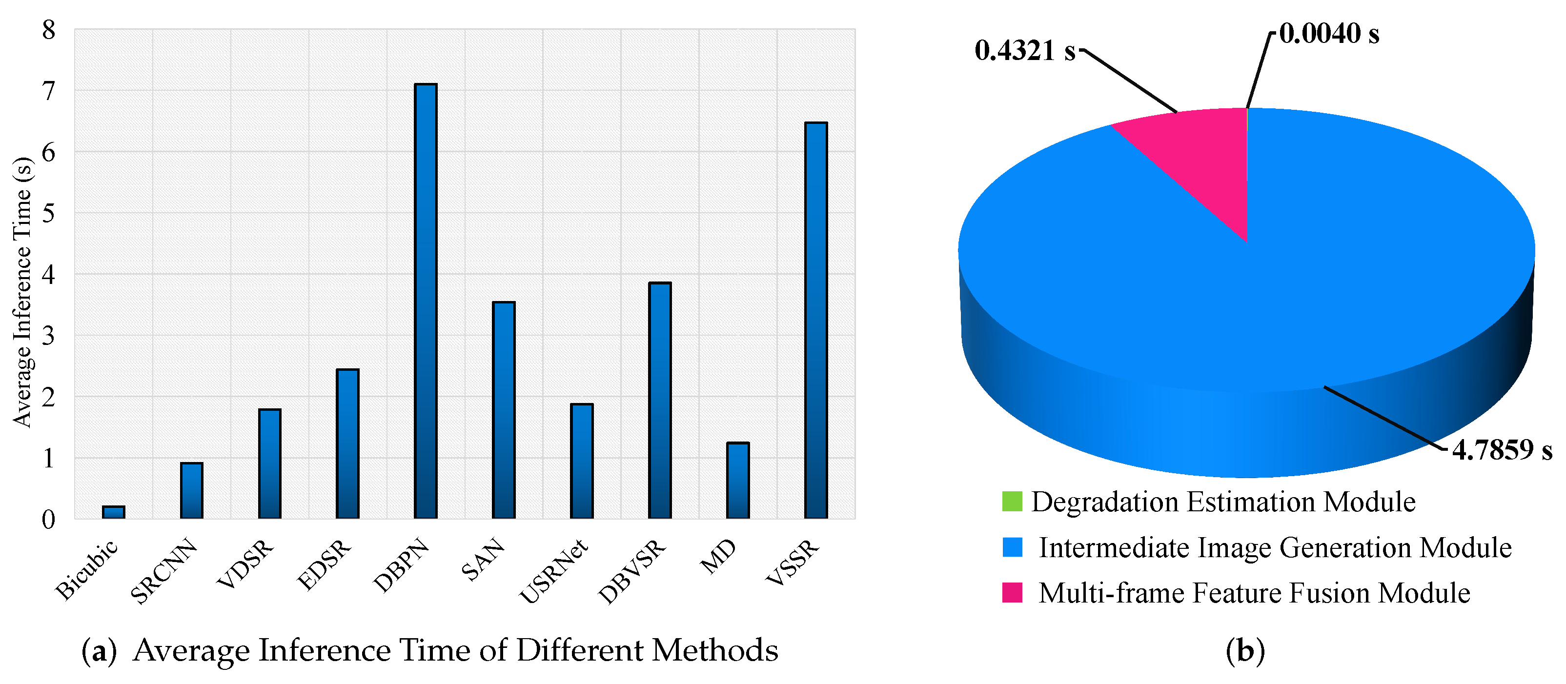
Moreover, the average inference time of various methods for reconstructing the San-ya scene is shown in Figure 11a, from which we can observe that Bicubic is the fastest in all the methods, while SRCNN and cost less time than other DL-based methods. The reason is that an efficient interpolation pattern is used in Bicubic, and the network structures of SRCNN and are much simpler than other methods. It can also be observed from Figure 11a that VDSR, EDSR, and USRNet spend more time than SRCNN and , but much faster than DBVSR. This is due to the fact that SRCNN and use only 3 and 4 convolution layers, respectively, while VDSR, EDSR, and USRNet use multiple convolutional layers and residual connections, multiple residual blocks, and multiple U-net blocks, respectively. Moreover, DBPN is slower than other methods, while the inference time of VSSR is moderate (i.e., less than 7 s) among all the comparison methods. Therefore, the proposed VSSR can be effectively adopted to practical application. Furthermore, Figure 11b compares the average inference time of each module in the VSSR for reconstructing the San-ya scene with size 1280 × 1280. We can observe from Figure 11b that the degradation estimation module consumes the least amount of time (i.e., 0.0040 s), and the intermediate image generation module consumes the most time (i.e., 4.7859 s). It should be noted that the total time of the above three modules is less than the average inference time of VSSR shown in Figure 11a. This is because Figure 11b does not count the data import time and the time to store the results as images.
3.3. Experimental Results on the OVS-1 Data
To further examine the practicability of VSSR in real scenarios, we perform an additional group of experiments on OVS-1 data. Different from the Jilin-1 data, which utilizes 10 Jilin-1 videos for producing the LR-HR training pairs, the LR frames from OVS-1 data are directly fed into the networks trained without using any OVS-1 data. The visual performance of different methods is compared in Figure 12 and Figure 13, while the detailed evaluation results are shown in Table 3.
From these results, we can observe that the quality of SR results is better than the original LR frames. For instance, as shown in Figure 12, the details of the LR frame are very blurry, while the clarity of the HR frames obtained by various SR methods is improved to a certain extent. Similar phenomenon can also be found in the Marseille video (see Figure 13). It is worth stressing that when inputting a lower image spatial resolution, the accuracy obtained by using DL-based methods will also be lower. For example, the spatial resolution of OVS-1 data is 0.98 m less than that of Jilin-1 data, and the PSNR obtained is about 8 dB lower than that of Jilin-1 data. As displayed in Table 3, Bicubic provides worse results than other methods. The DL-based methods, which combine learning-based methods with model-based ones under the MAP framework (i.e., USRNet, DBVSR, and VSSR), outperform the comparison methods without fully considering the degradation process. Moreover, MISR-based methods (i.e., DBVSR and VSSR) yield superior performance than SISR-based methods (i.e., SRCNN, VDSR, EDSR, DBPN, SAN, USRNet, and ). For instance, it is notable from Table 3 that the evaluation indexes of DBVSR and VSSR achieve the second-best and best performance among all methods. As plotted in Figure 12 and Figure 13, the visual results of DBVSR and VSSR are more realistic and clearer than other methods. The reasons for good results of VSSR are that it integrates the advantages of both learning-based and model-based methods by splitting the SR problem into two sub-optimization problems, and the blur kernel and noise level is flexibly estimated. Last but not least, the spatial-temporal information of neighboring frames are fully considered by 3D residual blocks. In a nutshell, the VSSR outperforms the comparison methods in restoring realistic SR results.
3.4. Ablation Study
Ablation experiments are designed in this subsection to assess the advantages of the proposed VSSR. All the experiments are conducted on the San-ya video from the Jilin-1 data.
In our ablation study, the effectiveness of each module (i.e., degradation estimation module, intermediate image generation module, and multi-frame feature fusion module) are examined. To that end, the modules in VSSR are gradually removed to evaluate the change in PSNR and SSIM. In greater detail, when the degradation estimation module is deleted from VSSR, fixed blur kernel and noise level are used rather than changing with the input LR frames. The fixed blur kernel and noise level are then fed into the intermediate image generation module, whose outputs are stacked and input into the to generate the final SR results. When the intermediate image generation module is removed, the degradation estimation module will lose its efficacy. Motivated by the SRCNN and VDSR, each LR frame is upsampled by bicubic interpolation, and then those upsampled frames are fed into the multi-frame feature fusion module to produce the SR results. When the multi-frame feature fusion module is removed from VSSR, the of the center frame is taken as SR results.
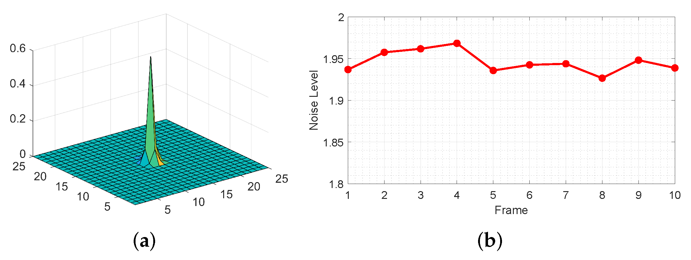
Note that the degradation estimation module is important in the VSSR, we visualize the estimated blur kernel and noise level obtained by the degradation estimation module in Figure 14. The estimated blur kernel is shown in Figure 14a, from which we can observe that all the 10 frames have the same standard deviation value (i.e., 0.5). The estimated noise level is depicted in Figure 14b, which demonstrates that the noise level of different frames fluctuates in a small range between 1.92 and 1.97. Moreover, the PSNR and SSIM of the above-mentioned methods are compared in Table 4, from which one can observe that both PSNR and SSIM will drop in case one of the modules is removed. Moreover, the performance is the worst when the intermediate image generation module is discarded. Based on the aforementioned analysis, all three modules are important to the VSSR.
3.5. Sensitivity Analysis of Different Parameters
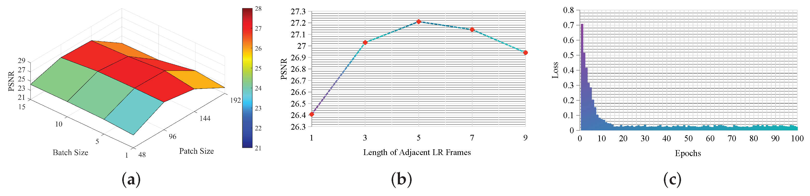
The sensitivity of several free parameters, including patch size, batch size, the length of adjacent LR frames, and epochs during training the VSSR, are discussed in this subsection. Figure 15 plots the influence of the above-mentioned parameters on the performance of VSSR in the San-ya video.
We first analyze the sensitivity of patch size and batch size. The patch size is chosen from {48,96,144,192}, while the batch size is selected from {1,5,10,15}. As shown in Figure 15a, the performance of VSSR fluctuates with the change of patch size and batch size. As to the patch size, the PSNR will increase in case the patch size is larger than 48 and lower than 144. As to the batch size, the SR results are satisfactory when it equals to or is larger than 5. In the experiments, we set the patch size to 96 and the batch size to 5 to make a trade-off between the model effectiveness and efficiency.
We then discuss the influence of the length of neighboring LR frames T on the SR performance. The SR results are reconstructed with various length of LR sequences, i.e., {1,3,5,7,9}. In particular, it is observed from Figure 15b that when , VSSR degenerates to a SISR method, whose performance is inferior to . When T increases from 3 to 9, the PSNR slightly fluctuates in a small range. Notably that larger T will increase extra calculation burden, we set in the experiments.
Finally, the impact of epochs on the SR performance is analyzed. The loss versus training epochs is shown in Figure 15c, in which the epochs are varied from 1 to 100 with an interval of 1. It is clearly visible in Figure 15c that the loss drops rapidly in the first couple of epochs, then decreases slowly as epochs increasing, and finally tends to be stable. In the experiments, we train VSSR by using 50 epochs to generate a stable and effective model for SR of video satellite images.
4. Discussion
This paper aims to propose a model-based deep neural network for SR of video satellite images. The quality and clarity of video satellite images are improved, which is conducive to a wider application of video satellites in dynamic monitoring. In this section, we discuss the following issues.
First, we explain and discuss how the modules are trained. In the training process, we first train the degradation estimation module by using the loss term shown in Equation (8), and then the trained degradation estimation module is adopted to estimate the noise level and the standard deviation of , and the intermediate image generation module and multi-frame feature fusion module are optimized by using Equation (13). The reasons for full training the first module and then training the other two modules are: (1) Use the trained degradation estimation module can estimate more accurate than an untrained one; (2) The and estimated by the trained degradation estimation module can be directly utilized to train the intermediate image generation module and multi-frame feature fusion module. That means, we only need to optimize these two modules at the same time instead of three modules, which can speed up the training speed. As to the effectiveness of the VSSR on the training and test sets, It is shown in Figure 15c that the training loss tends to be stable after about 20 epochs and fluctuates in a narrow range around 0.03. Due to the different characteristics of different videos, the evaluation metric values (e.g., PSNR and SSIM) obtained by different training videos are different. As to the test set, the results are shown in Table 2 and Table 3. The accuracy also varies from video to video. For instance, the PSNR of San-ya, San Diego, and Macao is 27.0287, 26.1814, and 28.5170 dB, respectively.
Second, it should be noted that the proposed VSSR is an offline method rather than an online method. This is because it uses pre-acquired videos for training, while an online method continues to learn from live data. In the testing procedure, the whole trained VSSR is adopted to reconstruct the HR counterpart of the input LR frames. When new video data is acquired, the trained VSSR network can be treated as a pre-trained model, and then the pre-trained model is fine-tuned with the newly acquired data. Of course, the model can also be retrained with all the video data (i.e., pre-acquired and newly acquired data), but this will be more time-consuming.
Furthermore, there is still room for improvement. For instance, in our VSSR, a deep unfolding module based on two-dimensional wavelet-based U-net is designed to obtain the intermediate HR results, and a 3D feature fusion subnetwork is subsequently used to fuse features from adjacent frames. In other words, VSSR uses 2D wavelet-based U-net and 3D Resnet separately instead of directly using 3D wavelet-based U-net to obtain the final HR result. This is because when the number of feature maps n increases to 128, 256, or 512, 3D wavelet-based U-net will consume more calculation and storage space than its corresponding 2D version. However, if lightweight convolution models and wavelet-based U-net calculation methods can be proposed, it is worthwhile to directly adopt 3D wavelet-based U-net to obtain the final HR results in the future.
5. Conclusions
In this paper, a model-based deep neural network (i.e., VSSR) is particularly designed to perform SR on video satellite images. In contrast to existing DL-based methods, which do not fully consider the degradation process when mapping the relationship between LR frames and their HR counterparts, the proposed VSSR integrates the advantages of learning-based methods with model-based ones by splitting the objective function of the degradation model into two sub-optimization problems. By constructing a degradation estimation module, both blur kernel and noise level are flexibly estimated and varied with the input data instead of manually setting those parameters in advance. Intermediate image generation module plays a vital role to deal with the sub-optimization problems, one of which has analytical solution while the other can be solved by a wavelet-based U-net (i.e., ). The main contribution of the multi-frame feature fusion module is to fuse the spatial-temporal information from multiple video frames by using 3D residual blocks. Experiments are performed on both Jilin-1 and OVS-1 data. The visual results have demonstrated that HR frames generated by VSSR contain sharper edges, fewer artifacts, and clearer visual effects than comparison methods. Moreover, the SR results are also quantitatively evaluated by 5 evaluation metrics. It is worth underlining that the proposed VSSR yields higher PSNR, CC, SSIM and lower RMSE and ERGAS than state-of-the-art methods. The proposed method could be of great interest for a wider application of video satellites. Future research can be conducted to design lightweight networks for SR of video satellite images. Studying in-depth the impact of resolution, bit depth, file format on image quality is also very promising. Additional studies are also needed in future to optimize the network structure by neural architecture search.
Author Contributions
Conceptualization, Z.H. and X.L.; methodology, Z.H.; software, Z.H.; validation, Z.H., X.L. and R.Q.; formal analysis, R.Q.; resources, Z.H.; data curation, Z.H.; writing—original draft preparation, Z.H.; writing—review and editing, X.L. and R.Q.; project administration, Z.H.; funding acquisition, Z.H. All authors have read and agreed to the published version of the manuscript.
Funding
This research was funded by the National Key Research and Development Program of China under grant number 2020YFA0714103, the National Key Laboratory of Science and Technology on Automatic Target Recognition under grant number WDZC20205500205, the Innovation Group Project of Southern Marine Science and Engineering Guangdong Laboratory (Zhuhai) under grant number 311021018, the Key-Area Research and Development Program of Guangdong Province under grant number 2020B0202010002, the Guangdong Basic and Applied Basic Research Foundation under grant number 2019A1515011877, the Fundamental Research Funds for the Central Universities under grant number 19lgzd10, and the Guangzhou Science and Technology Planning Project under grant number 202002030240.
Institutional Review Board Statement
Not applicable.
Informed Consent Statement
Not applicable.
Data Availability Statement
The Jilin-1 data in this study are openly and freely available at http://charmingglobe.com/ (accessed on 10 September 2021). The OVS-1 data in this study are openly and freely available at https://www.myorbita.net/index.aspx (accessed on 10 September 2021). The 30 additional videos are openly and freely available at https://pixabay.com/videos (accessed on 1 October 2021).
Acknowledgments
The authors would like to thank Chang Guang Satellite Technology Co., Ltd. for providing the Jilin-1 video datasets and Zhuhai Orbita Aerospace Science & Technology Co., Ltd. for providing the Zhuhai-1 video datasets.
Conflicts of Interest
The authors declare no conflict of interest.
References
- Yang, T.; Wang, X.; Yao, B.; Li, J.; Zhang, Y.; He, Z.; Duan, W. Small moving vehicle detection in a satellite video of an urban area. Sensors 2016, 16, 1528. [Google Scholar] [CrossRef] [PubMed] [Green Version]
- Wang, Y.; Wang, T.; Zhang, G.; Cheng, Q.; Wu, J.Q. Small target tracking in satellite videos using background compensation. IEEE Trans. Geosci. Remote Sens. 2020, 58, 7010–7021. [Google Scholar] [CrossRef]
- Zhang, S.; Yuan, Q.; Li, J. Video satellite imagery super resolution for ‘Jilin-1’ via a single-and-multi frame ensembled framework. In Proceedings of the 2020 IEEE International Geoscience and Remote Sensing Symposium (IGARSS), Waikoloa, HI, USA, 26 September–2 October 2020; pp. 2731–2734. [Google Scholar]
- Gu, Y.; Wang, T.; Jin, X.; Gao, G. Detection of event of interest for satellite video understanding. IEEE Trans. Geosci. Remote Sens. 2020, 58, 7860–7871. [Google Scholar] [CrossRef]
- Benzenati, T.; Kallel, A.; Kessentini, Y. Two stages pan-sharpening details injection approach based on very deep residual networks. IEEE Trans. Geosci. Remote Sens. 2021, 59, 4984–4992. [Google Scholar] [CrossRef]
- Babcock, C.; Finley, A.O.; Looker, N. A Bayesian model to estimate land surface phenology parameters with harmonized Landsat 8 and Sentinel-2 images. Remote Sens. Environ. 2021, 261, 112471. [Google Scholar] [CrossRef]
- Iyer, G.; Chanussot, J.; Bertozzi, A.L. A graph-based approach for data fusion and segmentation of multimodal images. IEEE Trans. Geosci. Remote Sens. 2021, 59, 4419–4429. [Google Scholar] [CrossRef]
- Gao, H.; Yang, Y.; Li, C.; Gao, L.; Zhang, B. Multiscale residual network with mixed depthwise convolution for hyperspectral image classification. IEEE Trans. Geosci. Remote Sens. 2021, 59, 3396–3408. [Google Scholar] [CrossRef]
- Li, H.; Man, Y. Moving ship detection based on visual saliency for video satellite. In Proceedings of the 2016 IEEE International Geoscience and Remote Sensing Symposium (IGARSS), Beijing, China, 10–15 July 2016; pp. 1248–1250. [Google Scholar]
- Xuan, S.; Li, S.; Han, M.; Wan, X.; Xia, G.S. Object tracking in satellite videos by improved correlation filters with motion estimations. IEEE Trans. Geosci. Remote Sens. 2020, 58, 1074–1086. [Google Scholar] [CrossRef]
- Zhang, X.; Xiang, J. Moving object detection in video satellite image based on deep learning. LIDAR Imaging Detection and Target Recognition 2017. In Proceedings of the International Society for Optics and Photonics, Changchun, China, 23–25 July 2017; Volume 10605, p. 106054H. [Google Scholar]
- Park, S.C.; Park, M.K.; Kang, M.G. Super-resolution image reconstruction: A technical overview. IEEE Signal Process. Mag. 2003, 20, 21–36. [Google Scholar] [CrossRef] [Green Version]
- Yang, W.; Zhang, X.; Tian, Y.; Wang, W.; Xue, J.H.; Liao, Q. Deep learning for single image super-resolution: A brief review. IEEE Trans. Multimed. 2019, 21, 3106–3121. [Google Scholar] [CrossRef] [Green Version]
- Wang, Z.; Chen, J.; Hoi, S.C. Deep learning for image super-resolution: A survey. IEEE Trans. Pattern Anal. Mach. Intell. 2021, 43, 3365–3387. [Google Scholar] [CrossRef] [Green Version]
- Mallat, S.; Yu, G. Super-resolution with sparse mixing estimators. IEEE Trans. Image Process. 2010, 19, 2889–2900. [Google Scholar] [CrossRef] [Green Version]
- Zhang, L.; Chen, D.; Ma, J.; Zhang, J. Remote-sensing image superresolution based on visual saliency analysis and unequal reconstruction networks. IEEE Trans. Geosci. Remote Sens. 2020, 58, 4099–4115. [Google Scholar] [CrossRef]
- Yu, Y.; Li, X.; Liu, F. E-DBPN: Enhanced deep back-projection networks for remote sensing scene image superresolution. IEEE Trans. Geosci. Remote Sens. 2020, 58, 5503–5515. [Google Scholar] [CrossRef]
- Dong, R.; Zhang, L.; Fu, H. RRSGAN: Reference-based super-resolution for remote sensing image. IEEE Trans. Geosci. Remote Sens. 2021, 60, 5601117. [Google Scholar] [CrossRef]
- Faramarzi, E.; Rajan, D.; Christensen, M.P. Unified blind method for multi-image super-resolution and single/multi-image blur deconvolution. IEEE Trans. Image Process. 2013, 22, 2101–2114. [Google Scholar] [CrossRef] [PubMed]
- Molini, A.B.; Valsesia, D.; Fracastoro, G.; Magli, E. Deep learning for super-resolution of unregistered multi-temporal satellite images. In Proceedings of the 10th Workshop on Hyperspectral Imaging and Signal Processing: Evolution in Remote Sensing (WHISPERS), Amsterdam, The Netherlands, 24–26 September 2019; pp. 1–5. [Google Scholar]
- Salvetti, F.; Mazzia, V.; Khaliq, A.; Chiaberge, M. Multi-image super resolution of remotely sensed images using residual attention deep neural networks. Remote Sens. 2020, 12, 2207. [Google Scholar] [CrossRef]
- Chantas, G.K.; Galatsanos, N.P.; Woods, N.A. Super-resolution based on fast registration and maximum a posteriori reconstruction. IEEE Trans. Image Process. 2007, 16, 1821–1830. [Google Scholar] [CrossRef] [PubMed] [Green Version]
- Shen, H.; Zhang, L.; Huang, B.; Li, P. A MAP approach for joint motion estimation, segmentation, and super resolution. IEEE Trans. Image Process. 2007, 16, 479–490. [Google Scholar] [CrossRef]
- Irmak, H.; Akar, G.B.; Yuksel, S.E. A map-based approach for hyperspectral imagery super-resolution. IEEE Trans. Image Process. 2018, 27, 2942–2951. [Google Scholar] [CrossRef] [PubMed]
- Hou, H.; Andrews, H. Cubic splines for image interpolation and digital filtering. IEEE Trans. Acoust. Speech Signal Process. 1978, 26, 508–517. [Google Scholar]
- Liu, J.; Gan, Z.; Zhu, X. Directional bicubic interpolation-a new method of image super-resolution. In Proceedings of the 3rd International Conference on Multimedia Technology (ICMT-13), Guangzhou, China, 29 November–1 December 2013. [Google Scholar]
- Sun, J.; Xu, Z.; Shum, H.Y. Image super-resolution using gradient profile prior. In Proceedings of the IEEE Conference on Computer Vision and Pattern Recognition (CVPR), Anchorage, AK, USA, 23–28 June 2008; pp. 1–8. [Google Scholar]
- Shao, W.Z.; Deng, H.S.; Wei, Z.H. A posterior mean approach for MRF-based spatially adaptive multi-frame image super-resolution. Signal Image Video Process. 2015, 9, 437–449. [Google Scholar] [CrossRef]
- Ren, C.; He, X.; Pu, Y.; Nguyen, T.Q. Enhanced non-local total variation model and multi-directional feature prediction prior for single image super resolution. IEEE Trans. Image Process. 2019, 28, 3778–3793. [Google Scholar] [CrossRef] [PubMed]
- Mofidi, M.; Hajghassem, H.; Afifi, A. An adaptive parameter estimation in a BTV regularized image super-resolution reconstruction. Adv. Electr. Comput. Eng. 2017, 17, 3–11. [Google Scholar] [CrossRef]
- Shao, Z.; Wang, L.; Wang, Z.; Deng, J. Remote sensing image super-resolution using sparse representation and coupled sparse autoencoder. IEEE J. Sel. Topics Appl. Earth Observ. Remote Sens. 2019, 12, 2663–2674. [Google Scholar] [CrossRef]
- Gao, L.; Hong, D.; Yao, J.; Zhang, B.; Gamba, P.; Chanussot, J. Spectral superresolution of multispectral imagery with joint sparse and low-rank learning. IEEE Trans. Geosci. Remote Sens. 2021, 59, 2269–2280. [Google Scholar] [CrossRef]
- Li, X.; Zhang, Y.; Ge, Z.; Cao, G.; Shi, H.; Fu, P. Adaptive nonnegative sparse representation for hyperspectral image super-resolution. IEEE J. Sel. Top. Appl. Earth Observ. Remote Sens. 2021, 14, 4267–4283. [Google Scholar] [CrossRef]
- Dong, C.; Loy, C.C.; He, K.; Tang, X. Image super-resolution using deep convolutional networks. IEEE Trans. Pattern Anal. Mach. Intell. 2016, 38, 295–307. [Google Scholar] [CrossRef] [Green Version]
- Kim, J.; Lee, J.K.; Lee, K.M. Accurate image super-resolution using very deep convolutional networks. In Proceedings of the IEEE Conference on Computer Vision and Pattern Recognition (CVPR), Las Vegas, NV, USA, 27–30 June 2016; pp. 1646–1654. [Google Scholar]
- Lim, B.; Son, S.; Kim, H.; Nah, S.; Mu Lee, K. Enhanced deep residual networks for single image super-resolution. In Proceedings of the IEEE Conference on Computer Vision and Pattern Recognition (CVPR), Honolulu, HI, USA, 21–26 July 2017; pp. 136–144. [Google Scholar]
- Haris, M.; Shakhnarovich, G.; Ukita, N. Deep back-projection networks for super-resolution. In Proceedings of the IEEE Conference on Computer Vision and Pattern Recognition (CVPR), Salt Lake City, UT, USA, 18–23 June 2018; pp. 1664–1673. [Google Scholar]
- Dai, T.; Cai, J.; Zhang, Y.; Xia, S.T.; Zhang, L. Second-order attention network for single image super-resolution. In Proceedings of the IEEE Conference on Computer Vision and Pattern Recognition (CVPR), Long Beach, CA, USA, 15–20 June 2019; pp. 11065–11074. [Google Scholar]
- Luo, Y.; Zhou, L.; Wang, S.; Wang, Z. Video satellite imagery super resolution via convolutional neural networks. IEEE Geosci. Remote Sens. Lett. 2017, 14, 2398–2402. [Google Scholar] [CrossRef]
- Xiao, A.; Wang, Z.; Wang, L.; Ren, Y. Super-resolution for “Jilin-1” satellite video imagery via a convolutional network. Sensors 2018, 18, 1194. [Google Scholar] [CrossRef] [Green Version]
- Jiang, K.; Wang, Z.; Yi, P.; Jiang, J. A progressively enhanced network for video satellite imagery superresolution. IEEE Signal Process. Lett. 2018, 25, 1630–1634. [Google Scholar] [CrossRef]
- Jiang, K.; Wang, Z.; Yi, P.; Jiang, J.; Xiao, J.; Yao, Y. Deep distillation recursive network for remote sensing imagery super-resolution. Remote Sens. 2018, 10, 1700. [Google Scholar] [CrossRef] [Green Version]
- Jiang, K.; Wang, Z.; Yi, P.; Wang, G.; Lu, T.; Jiang, J. Edge-enhanced GAN for remote sensing image superresolution. IEEE Trans. Geosci. Remote Sens. 2019, 57, 5799–5812. [Google Scholar] [CrossRef]
- Pan, J.; Cheng, S.; Zhang, J.; Tang, J. Deep blind video super-resolution. arXiv 2020, arXiv:2003.04716. [Google Scholar]
- Zhang, K.; Gool, L.V.; Timofte, R. Deep unfolding network for image super-resolution. In Proceedings of the IEEE Conference on Computer Vision and Pattern Recognition (CVPR), Virtual, 14–19 June 2020; pp. 3217–3226. [Google Scholar]
- Ronneberger, O.; Fischer, P.; Brox, T. U-net: Convolutional networks for biomedical image segmentation. In Proceedings of the International Conference on Medical Image Computing and Computer-Assisted Intervention, Munich, Germany, 5–9 October 2015; pp. 234–241. [Google Scholar]
- Liu, P.; Zhang, H.; Lian, W.; Zuo, W. Multi-level wavelet convolutional neural networks. IEEE Access 2019, 7, 74973–74985. [Google Scholar] [CrossRef]
- Chen, G.; Zhu, F.; Ann Heng, P. An efficient statistical method for image noise level estimation. In Proceedings of the IEEE International Conference on Computer Vision (ICCV), Santiago, Chile, 7–13 December 2015; pp. 477–485. [Google Scholar]
- Lin, T.Y.; RoyChowdhury, A.; Maji, S. Bilinear CNN models for fine-grained visual recognition. In Proceedings of the IEEE International Conference on Computer Vision (ICCV), Santiago, Chile, 7–13 December 2015; pp. 1449–1457. [Google Scholar]
- Simonyan, K.; Zisserman, A. Very deep convolutional networks for large-scale image recognition. arXiv 2014, arXiv:1409.1556. [Google Scholar]
- Nair, V.; Hinton, G.E. Rectified linear units improve restricted boltzmann machines. In Proceedings of the 27th International Conference on Machine Learning (ICML-10), Haifa, Israel, 21–24 June 2010; pp. 807–814. [Google Scholar]
- Glorot, X.; Bordes, A.; Bengio, Y. Deep sparse rectifier neural networks. In Proceedings of the Fourteenth International Conference on Artificial Intelligence and Statistics, Fort Lauderdale, FL, USA, 11–13 April 2011; pp. 315–323. [Google Scholar]
- Kingma, D.P.; Ba, J. Adam: A method for stochastic optimization. arXiv 2014, arXiv:1412.6980. [Google Scholar]
Figure 1.
The overall architecture of the proposed VSSR method.

Figure 2.
Architectures of the blur kernel estimation subnetwork .

Figure 3.
Architectures of the wavelet-based denoise subnetwork with corresponding number of feature maps (n), padding (p) size, and dilation (d) size. The kernel size and stride size of all the 2D convolution layers are set to 3 and 1, respectively.
Figure 3.
Architectures of the wavelet-based denoise subnetwork with corresponding number of feature maps (n), padding (p) size, and dilation (d) size. The kernel size and stride size of all the 2D convolution layers are set to 3 and 1, respectively.

Figure 4.
Architectures of the , , , h, , , and used in with corresponding number of feature maps (n), padding (p) size, and dilation (d) size. The kernel size and stride size of all the 2D convolution layers are set to 3 and 1, respectively. (a) . (b) . (c) . (d) h. (e) . (f) . (g) .
Figure 4.
Architectures of the , , , h, , , and used in with corresponding number of feature maps (n), padding (p) size, and dilation (d) size. The kernel size and stride size of all the 2D convolution layers are set to 3 and 1, respectively. (a) . (b) . (c) . (d) h. (e) . (f) . (g) .

Figure 5.
Architectures of the 3D feature fusion subnetwork with corresponding number of feature maps (n), padding (p) size, and dilation (d) size. The kernel size and stride size of all the 3D convolution layers are set to 3 and 1, respectively.
Figure 5.
Architectures of the 3D feature fusion subnetwork with corresponding number of feature maps (n), padding (p) size, and dilation (d) size. The kernel size and stride size of all the 3D convolution layers are set to 3 and 1, respectively.

Figure 6.
16 feature maps extracted by the eighth 3D residual block of for the San-ya data.

Figure 7.
Reconstruction results on the third frame of San-ya (Jilin-1 data) by the scale factor of ×4.
Figure 7.
Reconstruction results on the third frame of San-ya (Jilin-1 data) by the scale factor of ×4.

Figure 8.
Reconstruction results on the third frame of San Diego (Jilin-1 data) by the scale factor of ×4.
Figure 8.
Reconstruction results on the third frame of San Diego (Jilin-1 data) by the scale factor of ×4.

Figure 9.
Reconstruction results on the third frame of Macao (Jilin-1 data) by the scale factor of ×4.
Figure 9.
Reconstruction results on the third frame of Macao (Jilin-1 data) by the scale factor of ×4.

Figure 10.
Comparisons of the VSSR against other DL-based approaches. (a) compares the number of parameters. (b) compares the FLOPs when we acquit a 1280 × 1280 video frame. (a) Parameters and PSNR. (b) FLOPs and PSNR.
Figure 10.
Comparisons of the VSSR against other DL-based approaches. (a) compares the number of parameters. (b) compares the FLOPs when we acquit a 1280 × 1280 video frame. (a) Parameters and PSNR. (b) FLOPs and PSNR.

Figure 11.
Comparison of the average inference time for reconstructing the San-ya scene from the Jilin-1 data. (a) compares the average inference time of different methods. (b) compares the average inference time of each module in the VSSR for reconstructing the San-ya scene with size 1280 × 1280. (a) Average Inference Time of Different Methods. (b) Average Inference Time of Each Module.

Figure 12.
Reconstruction results on the third frame of Dalian (OVS-1 data) by the scale factor of ×4.
Figure 12.
Reconstruction results on the third frame of Dalian (OVS-1 data) by the scale factor of ×4.

Figure 13.
Reconstruction results on the third frame of Milwaukee (OVS-1 data) by the scale factor of ×4.
Figure 13.
Reconstruction results on the third frame of Milwaukee (OVS-1 data) by the scale factor of ×4.

Figure 14.
Visualization of the estimated blur kernel and noise level obtained by the degradation estimation module on the San-ya data. (a) Estimated blur kernel. The standard deviation of all 10 frames is 0.5. (b) Estimated noise level. The noise level of different frames fluctuates in a small range between 1.92 and 1.97.

Figure 15.
Influence of parameters on the performance of VSSR in the San-ya video. (a) Influence of patch size and batch size. (b) Influence of the length of adjacent LR frames. (c) Influence of epochs during training the VSSR.
Figure 15.
Influence of parameters on the performance of VSSR in the San-ya video. (a) Influence of patch size and batch size. (b) Influence of the length of adjacent LR frames. (c) Influence of epochs during training the VSSR.


Table 1.
Jilin-1 and OVS-1 data used in the experiments.
| Satellite | Data | Train or Test | Duration(s) | Frame Size | Acquisition Time | Side Swing Angle |
|---|---|---|---|---|---|---|
| Jilin-1 | Adana-1 | Train | 30 | 1280 × 1280 | 25 May 2017 | 18.0424 |
| Adana-2 | Train | 30 | 1280 × 1280 | 25 May 2017 | 18.0424 | |
| Dubai | Train | 25 | 1280 × 1280 | Unknown | Unknown | |
| Libya-Del | Train | 30 | 1280 × 1280 | 20 May 2017 | 2.1256 | |
| Minneapolis-1 | Train | 30 | 1280 × 1280 | 2 June 2017 | 5.0133 | |
| Minneapolis-2 | Train | 30 | 1280 × 1280 | 2 June 2017 | 5.0133 | |
| Muharraq | Train | 30 | 1280 × 1280 | 4 June 2017 | 4.8243 | |
| San Francisco | Train | 20 | 1280 × 1280 | 24 April 2017 | 17.0168 | |
| Tunisia | Train | 30 | 1280 × 1280 | 25 May 2017 | 7.5114 | |
| Valencia | Train | 30 | 1280 × 1280 | 20 May 2017 | −6.6864 | |
| San-ya | Test | 9 | 1280 × 1280 | 19 December 2019 | Unknown | |
| San Diego | Test | 32 | 1280 × 1280 | 7 September 2017 | Unknown | |
| Macao | Test | 26 | 1280 × 1280 | 30 November 2019 | Unknown | |
| OVS-1 | Dalian | Test | 29 | 600 × 600 | 18 June 2017 | 0 |
| Marseille | Test | 34 | 600 × 600 | 23 April 2018 | 4 |
Table 2.
Quantitative evaluation of the proposed VSSR against different methods on the Jilin-1 data with scale factor of 4, Bold indicates the best and italic underline indicates the second-best performance.
Table 2.
Quantitative evaluation of the proposed VSSR against different methods on the Jilin-1 data with scale factor of 4, Bold indicates the best and italic underline indicates the second-best performance.
| Data | Metrics | Algorithms | |||||||||
|---|---|---|---|---|---|---|---|---|---|---|---|
| Bicubic | SRCNN | VDSR | EDSR | DBPN | SAN | USRNet | DBVSR | VSSR | |||
| San-ya | RMSE | 15.1337 | 14.4477 | 13.5625 | 13.4138 | 13.5207 | 13.2906 | 12.3862 | 12.1839 | 14.1121 | 11.2999 |
| PSNR | 24.4933 | 24.8664 | 25.4470 | 25.5372 | 25.4751 | 25.6055 | 26.2059 | 26.3800 | 25.0739 | 27.0287 | |
| CC | 0.9800 | 0.9814 | 0.9835 | 0.9839 | 0.9839 | 0.9841 | 0.9862 | 0.9874 | 0.9820 | 0.9887 | |
| SSIM | 0.8416 | 0.8285 | 0.8605 | 0.8461 | 0.8434 | 0.8564 | 0.8561 | 0.8697 | 0.8367 | 0.8943 | |
| ERGAS | 4.0471 | 3.8679 | 3.6266 | 3.5875 | 3.6151 | 3.5563 | 3.3157 | 3.2572 | 3.7776 | 3.0221 | |
| San Diego | RMSE | 16.5994 | 15.5076 | 15.0225 | 14.3624 | 14.6138 | 14.3030 | 13.3640 | 13.2555 | 15.2080 | 12.4872 |
| PSNR | 23.7130 | 24.2891 | 24.5785 | 24.9678 | 24.8144 | 24.9972 | 25.5826 | 25.6654 | 24.4592 | 26.1814 | |
| CC | 0.9722 | 0.9750 | 0.9767 | 0.9786 | 0.9782 | 0.9786 | 0.9815 | 0.9824 | 0.9758 | 0.9838 | |
| SSIM | 0.8462 | 0.8430 | 0.8614 | 0.8605 | 0.8497 | 0.8680 | 0.8480 | 0.8687 | 0.8503 | 0.8976 | |
| ERGAS | 5.7135 | 5.3339 | 5.1703 | 4.9430 | 5.0284 | 4.9208 | 4.5970 | 4.5627 | 5.2309 | 4.2971 | |
| Macao | RMSE | 12.9320 | 12.4416 | 11.7892 | 11.3623 | 11.7063 | 10.9831 | 10.2995 | 10.1468 | 11.9849 | 9.5578 |
| PSNR | 25.8895 | 26.2109 | 26.6962 | 27.0099 | 26.7543 | 27.3025 | 27.8531 | 27.9965 | 26.5384 | 28.5170 | |
| CC | 0.9849 | 0.9860 | 0.9872 | 0.9882 | 0.9879 | 0.9889 | 0.9903 | 0.9914 | 0.9867 | 0.9919 | |
| SSIM | 0.8582 | 0.8385 | 0.8707 | 0.8638 | 0.8559 | 0.8793 | 0.8794 | 0.8805 | 0.8496 | 0.9085 | |
| ERGAS | 2.8356 | 2.7283 | 2.5848 | 2.4915 | 2.5668 | 2.4083 | 2.2585 | 2.2244 | 2.6281 | 2.0957 | |
Table 3.
Quantitative evaluation of the proposed VSSR against different methods on the OVS-1 data with scale factor of 4, Bold indicates the best and italic underline indicates the second-best performance.
Table 3.
Quantitative evaluation of the proposed VSSR against different methods on the OVS-1 data with scale factor of 4, Bold indicates the best and italic underline indicates the second-best performance.
| Data | Metrics | Algorithms | |||||||||
|---|---|---|---|---|---|---|---|---|---|---|---|
| Bicubic | SRCNN | VDSR | EDSR | DBPN | SAN | USRNet | DBVSR | VSSR | |||
| Dalian | RMSE | 29.0069 | 28.8828 | 28.2472 | 28.1543 | 28.1097 | 27.7297 | 27.3340 | 26.9428 | 28.6239 | 26.5475 |
| PSNR | 18.8613 | 18.8946 | 19.0914 | 19.1178 | 19.1307 | 19.2475 | 19.3675 | 19.4992 | 18.9728 | 19.6274 | |
| CC | 0.9292 | 0.9295 | 0.9325 | 0.9329 | 0.9334 | 0.9349 | 0.9369 | 0.9394 | 0.9305 | 0.9407 | |
| SSIM | 0.6612 | 0.6289 | 0.6791 | 0.6582 | 0.6730 | 0.6823 | 0.6667 | 0.7022 | 0.6450 | 0.7212 | |
| ERGAS | 8.1978 | 8.1631 | 7.9833 | 7.9568 | 7.9442 | 7.8375 | 7.7263 | 7.6145 | 8.0900 | 7.5033 | |
| Marseille | RMSE | 30.1338 | 29.7721 | 29.2010 | 29.1191 | 29.0149 | 28.6557 | 28.0308 | 27.7586 | 29.2474 | 27.1236 |
| PSNR | 18.4355 | 18.5187 | 18.7041 | 18.7209 | 18.7532 | 18.8555 | 19.0490 | 19.1397 | 18.6737 | 19.3361 | |
| CC | 0.9214 | 0.9224 | 0.9256 | 0.9257 | 0.9266 | 0.9280 | 0.9320 | 0.9335 | 0.9250 | 0.9359 | |
| SSIM | 0.6957 | 0.6660 | 0.7111 | 0.6969 | 0.7022 | 0.7141 | 0.6545 | 0.7342 | 0.6890 | 0.7548 | |
| ERGAS | 9.5903 | 9.4790 | 9.2950 | 9.2690 | 9.2353 | 9.1231 | 8.9228 | 8.8354 | 9.3128 | 8.6361 | |
Table 4.
Results of the ablation study on evaluating the effectiveness of each module in VSSR, bold indicates the best and italic underline indicates the second-best performance. “✓” denotes the module is adopted while “✗” denotes the module is not adopted.
Table 4.
Results of the ablation study on evaluating the effectiveness of each module in VSSR, bold indicates the best and italic underline indicates the second-best performance. “✓” denotes the module is adopted while “✗” denotes the module is not adopted.
| Module | PSNR | SSIM | ||
|---|---|---|---|---|
| Degradation Estimation Module | Intermediate Image Generation Module | Multi-Frame Feature Fusion | ||
| ✗ | ✓ | ✓ | 26.7144 | 0.8587 |
| Loss Efficacy | ✗ | ✓ | 25.8017 | 0.8553 |
| ✓ | ✓ | ✗ | 26.8511 | 0.8648 |
| ✓ | ✓ | ✓ | 27.0287 | 0.8943 |
Publisher’s Note: MDPI stays neutral with regard to jurisdictional claims in published maps and institutional affiliations. |
© 2022 by the authors. Licensee MDPI, Basel, Switzerland. This article is an open access article distributed under the terms and conditions of the Creative Commons Attribution (CC BY) license (https://creativecommons.org/licenses/by/4.0/).
Share and Cite
MDPI and ACS Style
He, Z.; Li, X.; Qu, R. Video Satellite Imagery Super-Resolution via Model-Based Deep Neural Networks. Remote Sens. 2022, 14, 749. https://0-doi-org.brum.beds.ac.uk/10.3390/rs14030749
AMA Style
He Z, Li X, Qu R. Video Satellite Imagery Super-Resolution via Model-Based Deep Neural Networks. Remote Sensing. 2022; 14(3):749. https://0-doi-org.brum.beds.ac.uk/10.3390/rs14030749
Chicago/Turabian StyleHe, Zhi, Xiaofang Li, and Rongning Qu. 2022. "Video Satellite Imagery Super-Resolution via Model-Based Deep Neural Networks" Remote Sensing 14, no. 3: 749. https://0-doi-org.brum.beds.ac.uk/10.3390/rs14030749
Note that from the first issue of 2016, this journal uses article numbers instead of page numbers. See further details here.