
Shield Tunnel Convergence Diameter Detection Based on Self-Driven Mobile Laser Scanning
by
 , , and
Lei Xu
1,2 ,
,
Jian Gong
1, 
Jiaming Na
3 ,
,
Yuanwei Yang
4,
Zhao Tan
1,
Norbert Pfeifer
5 and
and
Shunyi Zheng
2,* 1
China Railway Design Corporation, Tianjin 300308, China
2
School of Remote Sensing and Information Engineering, Wuhan University, Wuhan 430079, China
3
College of Civil Engineering, Nanjing Forestry University, Nanjing 210037, China
4
School of Geosciences, Yangtze University, Wuhan 430100, China
5
Department of Geodesy and Geoinformation, Technische Universität Wien, 1040 Vienna, Austria
*
Author to whom correspondence should be addressed.
Remote Sens. 2022, 14(3), 767; https://0-doi-org.brum.beds.ac.uk/10.3390/rs14030767
Submission received: 22 January 2022
/
Revised: 1 February 2022
/
Accepted: 3 February 2022
/
Published: 7 February 2022
(This article belongs to the Special Issue Mapping and Monitoring of Civil Infrastructures Using LiDAR/Laser Scanning)
Abstract
:The convergence diameter of shield tunnels is detected by ellipse fitting or local curve fitting to cross-section points. However, the tunnel section, which is extruded by an external force, has an irregular elliptical shape, and the waist of the tunnel is often blocked by accessories, resulting in data loss. This study proposes a convergence diameter and radial dislocation detection method based on block-level fitting. The proposed method solves the accuracy degradation caused by the model error and point cloud incompletion. First, the noise points in the tunnel section point cloud are removed using the least trimmed squares method. Second, the tunnel transverse seam is then located using the image edge detection algorithm. Third, the endpoint of the convergence diameter is determined by making a specific segment the center and shifting the detector from the center to the pinpoint. Finally, the convergence diameter and radial dislocation are detected by the endpoints of the segments. The experimental results showed that the absolute detection accuracy of this method was better than 3 mm, and the repeated detection accuracy was better than 2 mm. This result is consistent with prior total station measurements, which are more suitable for practical engineering applications.
1. Introduction
Urban rail transit is one of the main modes of transportation in modern cities, and the subway is an essential form of urban rail transit. China is at the peak of its subway construction. By the end of 2020, subways accounted for more than 78% of all cities’ rail transit projects [1]. Tunnels are an essential part of subway pipelines, and shield tunnels are the main forms of underground structures in metro engineering. With the increase in service time, continuous changes in the geological environment, and aging of materials, the tunnel structure will inevitably produce certain diseases [2], especially in cities with soft soils such as Shanghai, Hangzhou, and Guangzhou in China. Owing to the concealment, complexity, and uncertainty of subway tunnel engineering, tunnel structural health has a critical impact on the safety of public life and social property [3,4]. Ensuring the safe and economic operation of subway tunnels in their design life cycle has become one of the most crucial problems in the engineering community. Therefore, conducting normalized detection of tunnel structural diseases in the stages of project construction and operation has become an imperative task.
Shield tunnels can be divided by their section shape: circular, arched, rectangular, and horseshoe. Among them, the circular structure lining is the most widely used because of its simple assembly, easy replacement, and good resistance to soil pressure. For circular tunnel structures, the two primary parameters are convergence diameter and radial dislocation. Tunnel diameter convergence refers to the length deviation between the actual diameter of the cross-section and the design diameter, which is the deformation of the tunnel structure due to various factors in the surrounding environment [5]. Radial dislocation refers to the height deviation of adjacent segments in the same shield ring at the transverse seam caused by, for example, construction factors, changes in the surrounding environment, and uneven settlement of the soil layer [6]. These two parameters directly reflect the external pressure distribution and tunnel deformation and directly change the structural performance and mechanical characteristics of segments in tunnel engineering. As a result, water leakage and segment cracking can occur, and the overall seismic performance of the tunnel is affected.
Traditional monitoring methods rely on manual measurements. However, inspectors can only conduct inspections within a limited skylight time to ensure normal operation of a subway. The average detection time is 2–2.5 h/day. Given this time limitation, inspectors can only focus on disease-prone areas, easily resulting in missed inspections [7,8]. In addition, blurred photos and inaccurate records were obtained because of the dark internal environment of the tunnel. Therefore, the overall detection efficiency of this method was inadequate. Mobile laser scanning (MLS) technology has the advantages of no contact and no external light source required and has higher precision and efficiency than traditional methods [9,10,11]. These characteristics make MLS technology widely recommended and adopted by many institutions and researchers to detect tunnel structure disease [12,13,14,15].
MLS-based detection methods for tunnel section convergence can be divided into ellipse fitting and local curve fitting methods.
1.1. Related Work on Ellipse Fitting Method
The ellipse fitting method generally considers the cross-section of the tunnel as an ellipse. The cross-section is then fitted to obtain parameters such as the horizontal diameter, ellipse long half axis, ellipse short half axis, and rotation angle. To achieve the aforementioned purpose, scholars have designed an MLS tunnel detection and measurement system for the continuous section scanning of subway tunnels. The geometric parameters of the section point cloud are obtained using an algebraic ellipse fitting method to achieve convergence detection [16,17]. Du et al. [18] used the iterative ellipse fitting method to filter the point cloud noise and fit the tunnel section contour, in which the ellipse fitting method used the random sample consensus algorithm. Walton et al. [19] discussed the feasibility of the ellipse fitting method in tunnel profile deformation analysis using a ground laser scanner. Danielle et al. [20] verified the feasibility of the algebraic ellipse fitting method for tunnel section convergence measurement. They proved that this method can resist partial random and systematic errors. The aforementioned methods are clear and simple to apply. Their main steps are to fit the shield tunnel section shape as an ellipse and then realize convergence deformation analysis. However, the deformed section of the tunnel structure was an irregular elliptical shape. This shape deformation was caused by the complexity and uncertainty of the external force distribution around the tunnel [21]. The obtained ellipse parameters were the result of obeying the overall optimal principle; however, deviations from the actual situation in local areas remained large. These caused a large detection error when calculating the convergence diameter. Thus, if an elliptic model is directly used for fitting, it can generate a large calculation error.
1.2. Problem Formulation of Local Curve Fitting Fitting Method
The local curve fitting method has better accuracy than the ellipse fitting method. Scholars have also used local conic curve fitting to solve this problem. The main process is to obtain the center of the tunnel section by using the ellipse fitting method. After segment point clouds on both sides of the center of the circle are in a certain range above and below the horizontal line, the parameters of the conic curve model are fitted. The convergence diameter is detected by calculating the intersection of the horizontal line at the center of a circle and the curves on both sides [22]. To an extent, this method can avoid the effects of model errors, but the tunnel lining is usually installed with various communication cables. The inner wall of the tunnel near the horizontal line of the circle center was typically blocked, resulting in the loss of point cloud data. Thus, the applicability of this method is limited by environmental factors. In addition, the aforementioned method to determine the convergence diameter position differs from that during manual detection. Manual verification of data cannot be conducted directly and cannot connect with the existing historical detection results of the operation and maintenance departments. These results can hinder the management and maintenance work of relevant departments. Thus, a fast, accurate, and efficient detection method must be explored further.
Notably, the key successes of tunnel parameter detection are choosing the most appropriate fitting method and smart filtering the big point cloud to obtain points for which fitting is applied. Therefore, data preprocessing is important. A shield tunnel is constructed with blocks as the basic units. Each block has a definite geometric shape; therefore, successful block-level segmentation can improve precision.
Inspired by the aforementioned discussions, this study proposes a solution to detect the convergence diameter and radial dislocation using the block fitting method. The main objectives are as follows: to (1) integrate a self-driven mobile laser scanning system for data generation, (2) propose an edge detection-based method for tunnel block segmentation, and (3) design a block fitting method for tunnel parameter detection.
2. Methods
The block fitting method proposed in this study uses a point cloud collected by the MLS system. The main aim of the method is to reduce the 3D point cloud into a 2D grayscale image, and the characteristics of the ring seam and transverse seam are identified by a digital image processing algorithm. The "clean" tunnel inner wall point cloud is obtained by filtering and denoising after extracting the corresponding cross-section point cloud from the seam features. Finally, the convergence diameter and radial dislocation values were detected by the block fitting method. The flowchart of this method is shown in Figure 1.
2.1. System Integration and Measurement Error Analysis
The self-driven mobile laser scanning (SDMLS) system designed to identify tunnel structure deformation (Figure 2). The programmable logic controller (PLC) trolley includes a high-precision laser scanner, odometer, inclinometer, industrial computer, and other sensors. The PLC trolley has an independent power source and can travel at a constant pace down the track. The running speed of the trolley may be modified between 1 and 5 km/h, with a consistent speed error of less than 0.3%. To establish the system operating settings and scanning parameters and control the trolley’s operation status, the acquisition and control software was installed on the tablet computer and connected to the system through a wireless local area network or network connection.
In this study, the scanning line section is assumed to be a tunnel cross-section, and the endpoint of the convergence diameter was computed using the transverse seam offset. This assumption has fixed and unintentional errors, which can be divided into two categories: helix and transverse seam errors.
- (1)
- Helix error
The scanner performs a 360° continuous rotation measurement perpendicular to the tunnel as the trolley moves along the line direction. The scanning survey line was suitably dispersed in a spiral line (Figure 2). As a result, the scanning line in the 3D space was not precisely perpendicular to the line direction but at a slight clamping angle. When the section point cloud is projected onto the 2D plane, this non-strict orthogonality phenomenon results in a projection error, with the highest error between the starting point and the end point of the survey line.
The laser scanner employed in this investigation was a Z + F PROFILER 9012, with a line scanning frequency of 200 lines per second. The time spent scanning a single segment was 0.005 s. The scanning had a brief waiting phase between adjacent survey lines when the scanner was turned on, the actual scanning duration of a single section was approximately s, and gaps between corresponding survey lines emerged (Figure 2). The helix error can be calculated using Equation (1).
where R is the tunnel radius and L is a quarter of the pitch of the scanning spiral line (Figure 2). When the carrier is traveling at 3 km/h, the distance between the start and end points of the scan line is mm. Given the tunnel’s inner radius of 2.7m, the calculation error according to Equation (1) is mm, which can be ignored.
This study also used another laser scanner, a Faro focus 350: line scanning frequency, 220 lines per second; actual scanning duration of a single section, approximately s; and calculation error, according to Equation (1), mm, which can also be ignored.
- (2)
- Transverse seam error
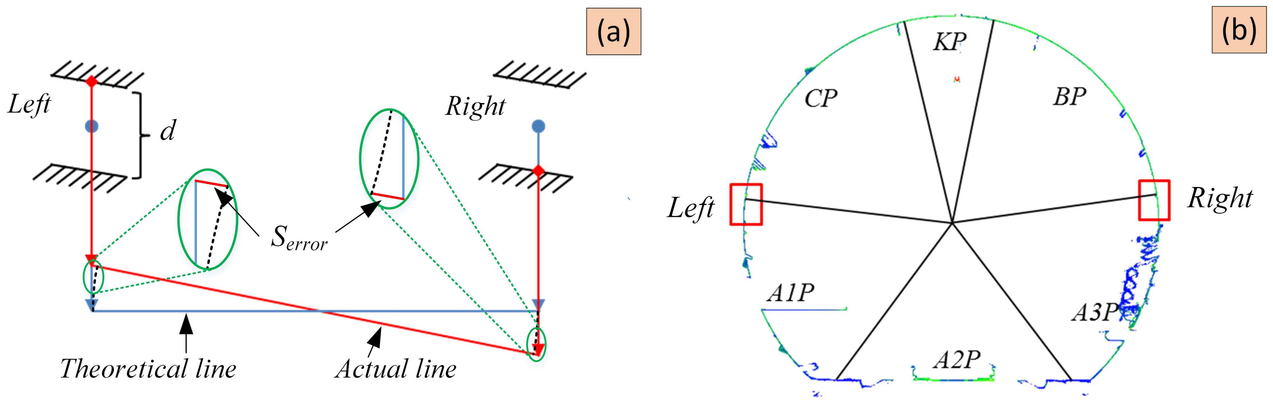
The location of the convergence diameter endpoint is determined by offsetting the center position of the given transverse seam on both sides; thus, the transverse seam position generates inaccuracy in the convergence diameter detection result. In the worst-case scenario, the transverse seams on the left and right sides are at the top and bottom of the seam, respectively (Figure 3). The inaccuracy produced by the convergence diameter detection result is the largest at this moment, and it may be calculated using Equation (2):
where is the design radius, and is the transverse seam width. The maximum error produced by the transverse seam positioning is mm, which is insignificant when the design radius is 2.7 m and the transverse seam width in the shield tunnel is approximately 1 cm, as shown in the preceding calculation
2.2. Point Cloud Mapping
2.2.1. Data Dimension Reduction
The point cloud collected by the SDMLS usually has a high density. If the original point cloud data are directly used to extract the seams of the shield segments, they require significant computer resources. Operation efficiency is also difficult to accept in engineering applications. Mapping 3D point clouds to 2D grayscale images can improve processing efficiency by reducing data dimensionality [23,24]. The original data obtained by the laser scanner usually include the horizontal angle, vertical angle, spatial distance, and reflection intensity of the target in the scanner coordinate system. To truly and intuitively describe the texture features of objects in the scene and facilitate the subsequent segment seam feature extraction, the reflection intensity of the laser points on the object surface is converted into the pixel value of the grayscale image.
The shield tunnel has the characteristics of a linear distribution and a nearly circular section; thus, the cylindrical model was used as the projection plane. In a single section, the geometric center of the tunnel section is used as the viewpoint. Based on the scanning angle, the image mapped by the laser points in the section can be regarded as an orthophoto. The distortion of its geometric features is negligible, and the projection conversion relationship between the laser points and pixels is simple and clear. The projection is convenient for subsequent feature extraction and conversion between the image and point cloud (Figure 4).
To improve the processing efficiency and control the projection error, the point cloud is projected into segments according to a certain interval (set as 20 m in this study). In a section of the point cloud, the approximate circle centers are calculated using the ellipse fitting method. The connecting line of the two centers, which are between the start and end of the interval, is used as the reference line. A cylindrical projection surface was constructed with the tunnel design radius as the projection radius. The cylindrical projection surface is spread into a 2D plane, and the scanning line is used as the unit for line-by-line projection, which is displayed as column pixels in order on the image. Each measuring point in the section is arranged according to the incident angle. Its position is represented by the ordinate Y, and the measuring line position is represented by the abscissa X. After determining the center and radius of the cylindrical projection circle and the horizontal and vertical resolutions of the projection orthophoto, the mapping can be calculated using Equation (3):
where represents the X coordinate corresponding to the laser point in the gray image; represents the Y coordinate corresponding to the laser point in the gray image; represents the cumulative distance between the measuring line where the laser point is located and the starting measuring line; indicates the set horizontal resolution; indicates that the section point cloud needs to be mapped to one half of the angle range value on the image; represents the radius of the projected cylinder; indicates the set vertical resolution; represents the incident angle of the laser point ; and represents the pixel value at .
For specific cases, the intersection point of the vertical line passing through the datum point and the cylindrical projection plane can be taken as the starting point, that is, the zero point of the Y coordinate in this image. The projection can be calculated point by point along the counterclockwise direction according to the advancing direction of the tunnel.
2.2.2. Feature Enhancement
The inner wall of the tunnel is made of concrete; thus, the corresponding laser reflectivity is basically the same. The grayscale image of the inner wall of the tunnel generated in the prior step shows that the overall color is dark, the change in light and shade in tone is small, and the characteristics of tunnel segment cracks are indistinct (such as in Figure 5). Therefore, the image must be further enhanced to ensure that the mapped grayscale image has a high contrast hue and obvious feature information. Histogram equalization is adopted in this case, that is, the distribution range of the pixel value is stretched to expand the range of two levels [25], as shown in Figure 5.
2.3. Seam Detection
The convergence diameter and radial dislocation detection in shield tunnels must be calculated and counted using the shield tunnel ring number. Therefore, accurate identification and positioning of tunnel segment cracks are the basis for subsequent data analysis. The shield segment is the general name of all blocks constituting the shield ring, specifically including three main types: standard block (A-type segment), adjacent block (B-type segment), and capping block (K-type segment). The standard block has a fixed size, whereas the capping block is small, generally 1/3–1/4 of the standard block. The size of the adjacent block adjacent to the capping block must be determined according to the actual needs. Generally, the common block mode of a subway tunnel is six blocks (3A + 2B + K) and seven blocks (4A + 2B + K).
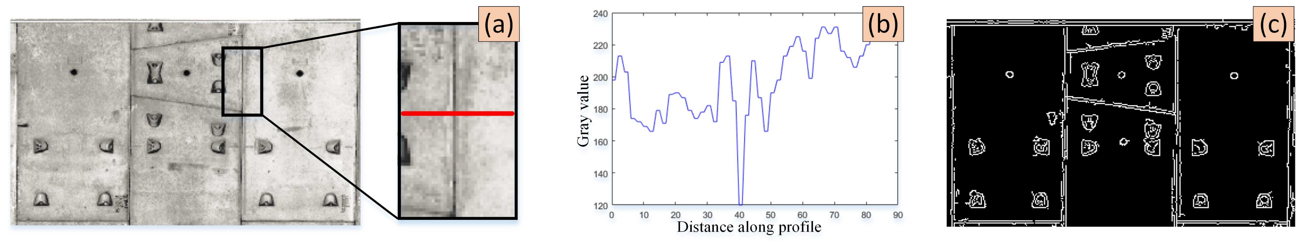
After the grayscale image is enhanced by histogram equalization, the segment seam shows significant changes in the brightness of local areas in the image; that is, the value changes sharply in a small local neighborhood (Figure 6). Therefore, the segment seam can be obtained by two processes: feature detection and extraction of grayscale images. Specifically, the combination of the Canny algorithm and Hough transform is used to identify and extract tunnel segment seams [26,27].
First, the Canny algorithm is used to detect the features of grayscale images [28]. The image edge features are obtained through Gaussian smoothing, gradient calculation, non-maximum suppression, and double-threshold detection. The extraction results are shown in Figure 6. The element composition in the resulting image remains complex because of the existence of block edges, namely: bolt holes and cable wires. Therefore, the Hough transform method was used to further separate the segment seams with line segment characteristics.
The number of line segments detected by the Hough transform is large, and the same segment seam may be detected as multiple discontinuous line segments because of environmental influences. In addition, line segments also contain much "noise" in non-seams, which requires further filtering and analysis to obtain accurate segment seams. In this study, filtering was performed based on the length and direction characteristics of the shield tunnel segment seams as follows:
In grayscale images, because the ring seams are distributed in a vertical line, the polar angle of the corresponding line segment detected is close to 180° or 0°. Therefore, the angle threshold can be set to traverse the line segment as a candidate for ring seams. Transverse seams appear or approach a horizontal linear distribution in the image; thus, the polar angle is close to 90° or 270°. However, because the pipelines on the inner wall of the tunnel also present a horizontal linear distribution, the transverse seams cannot be accurately obtained using the angle threshold. The lengths of the transverse seams are basically the same and are much smaller than the length of the pipeline; thus, the distance threshold is added. The straight-line segment that fulfills the requirements was selected as the candidate for the transverse seams. The ring seam and transverse seam can be defined by Equations (4) and (5), respectively.
where represents the extracted ring seams; is the extracted transverse seam; is the angle corresponding to the line segment; is the corresponding length of the line segment; is the pixel length corresponding to the width of the shield segment in the image; is the angle threshold of the ring seams, which is usually set to 1°; and is the angle threshold of the transverse seams, which is usually set to 3°.
After the aforementioned process, most of the obvious error line segments are filtered out (Figure 7), but many similar line segments around the seam interfere with the accurate positioning of the seam. Therefore, the next step is to use a statistical method to obtain the optimal seam position (Figure 7), by traversing the candidate line segments and line-by-segment statistics and selecting the line with the largest number of pixels as the initial ring seam (Figure 7).
After the initial value of the seam is obtained, the seams of the other segments are calculated according to the law of the splicing of shield segments. For ring seams, the horizontal axis of the other ring seams is obtained by recursing at equal intervals to the left and right sides according to the width of the segment. For transverse seams, other diameters are calculated along the inner direction of the ring according to the corresponding angles of the different types of segments. The recursive method is different according to the different shield tunnel segment assembly methods. For the continuous seam shield tunnel, the seam between the rings is continuous, and the seam can be extracted directly at equal intervals to the left and right sides according to the width of the segment. Stagger seam tunnels, according to the assembly requirements, usually show alternating and repeated distribution of segment seams. Therefore, transverse seams in the remaining shield rings can be based on the initial transverse seams according to the width of the segment. They are calculated twice at equal intervals.
2.4. Iterative Optimal Ellipse Fitting
Ellipse fitting parameters were calculated based on the 2D space. Before this step, the point cloud of the tunnel section must be accurately extracted and projected onto the 2D plane [29,30]. After the image coordinates of longitudinal seams of tunnels are obtained using the method described in Section 2.3, they are converted into corresponding survey line serial numbers. The corresponding survey line point clouds can then extracted.
At this time, pipes, cables, evacuation platforms, and other blocks installed on the inner wall of the tunnel, as well as dust floating in the environment, lead to many noise points in the section point cloud. If these noise points are not filtered or suppressed during processing, they will exert a significant impact on the accuracy of the results [10,31], as shown in blue in Figure 8. The data are not normally distributed, because of noise information in the tunnel section point cloud. When there are non-normal distribution errors (e.g., heavy-tailed errors), the fitting effect of the conventional least-squares method will be damaged. Therefore, the conventional least-squares method cannot be used for regression fitting.
In this study, the weighted least trimmed squares (LTS) method was used to fit the cross-section point cloud and resist the adverse effects of abnormal data. The LTS concept is a robust estimation method with a high breakdown point [32,33]. In the case of a large proportion of noise and gross error, it can also resist its adverse influence on regression analysis results and obtain a best fitting effect. However, experiments have shown that when the number of points involved in the fitting is large, a large amount of computation significantly reduces the computational efficiency. Therefore, this study designed a fast solution method based on the LTS concept. The designed method extracts m samples from n observations, with each sample randomly containing k observations, and uses k observations to solve the least square estimate δ. The squared residuals of n observations under δ conditions can then be obtained. They are arranged in ascending order. The sum of the squares of the h residuals is expressed as . Considering all the combinations of , the smallest pair response is the exact solution of the LTS estimate.
Based on the elliptic equation (Equation (6)), at least five observation points are required in a tunnel section to obtain the equation parameters. To avoid local fitting caused by the uneven distribution of selected observation values [34], the cross-section point cloud was divided in this study at 60° intervals. One point was selected from the other five parts, except the bottom part, to participate in the fitting to ensure that the calculated ellipse parameters approach the optimal value.
The repeated sampling number m is set to the number of subpoint clouds at each part. The fitting parameters of each group of samples are calculated . The residuals of n observations are squared and arranged in ascending order. The set of parameters with the smallest sum of the squares of the first h residuals is denoted as , and it is taken as the initial value of fitting.
The negative effects of noise and gross error are gradually eliminated by means of weight selection iteration, and the indirect adjustment model is used to calculate the adjustment of elliptic parameters. In the adjustment results, the correction values of the gross error and noise were too large. Using this characteristic, the weight of the observation value was adjusted according to the Danish weight function [35] (Equation (7)) and stopped until the set number of iterations was fulfilled or less than the set threshold.
where is the unit weight error obtained from Equation (8):
After obtaining the ellipse parameters, all the laser points are traversed in the current section, the orthogonal distance d is calculated with the fitting ellipse point by point, and the distance threshold is set. If , the laser point is included in the set of tunnel inner wall points; otherwise, it is a non-inner wall point and is excluded.
2.5. Block Fitting Detection
The process of detecting the convergence diameter based on the block fitting method is described in detail as follows. First, the segments are divided into rings and blocks based on the identified seams. Second, the noise points on the segment are filtered based on the radius threshold and iterative registration. Finally, the circular fitting segment point cloud is used to calculate the convergence diameter based on the fitting radius, ellipse center, and transverse seam position. The specific steps are as follows.
- (1)
- Noise filtering by model iterative registration
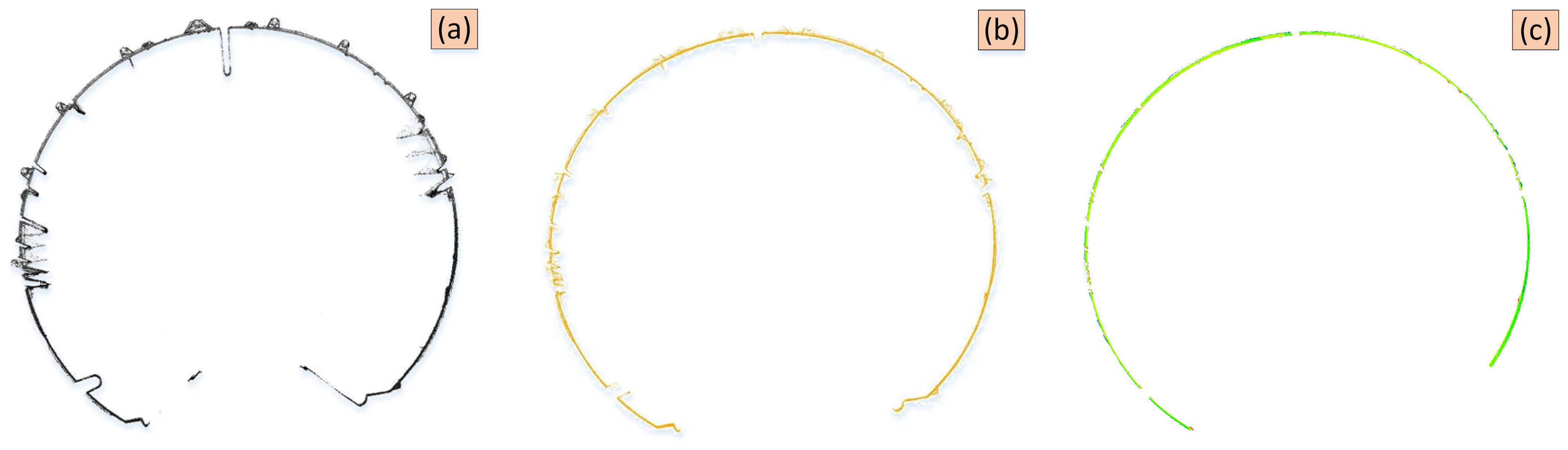
The corresponding shield ring point cloud was extracted according to the segment seam coordinates detected in Section 2.3. The point cloud was preliminarily filtered using the method described in Section 2.4 to remove the noise points such as the track plate and catenary, to improve the reliability of filtering in the next step. The effects before and after filtering are shown in Figure 9.
After preliminary filtering, the inner wall of the tunnel still had noise points, which mainly included various pipelines installed on the tunnel wall and bolt holes at segment connections (Figure 9). The verification of several engineering cases and the residuals after circular fitting prove that the segment seam is the weak position of the entire tunnel structure. The overall deformation of the tunnel is mainly due to the external force acting on the segment seam, resulting in dislocation between each segment. The rigid strength and stability of the segment structure are high, and generally, there is no deformation [36,37]. Based on the obtained knowledge of segment deformation, the cylindrical model of the shield segment is constructed, the segment block point cloud is iteratively registered with the model, and the distance from the point cloud to the model is calculated. The distance threshold for deformation δ is set. Noise filtering on the registered block point cloud is conducted to realize the fine filtering of the segment point cloud (Figure 10). These segment point clouds, after fine filtering, can improve the accuracy of the next circular fitting algorithm.
- (2)
- Circle fitting segment point cloud
The segment point cloud processed in step (1) is projected onto the 2D XOY plane. The x-axis straight-line direction of the plane is right, and the y-axis is vertically upward. The coordinate center is translated to the center point of the fitting ellipse of the section. On the basis of the 2D circular fitting algorithm, the fitted circular radius and center coordinates were obtained.
- (3)
- Calculation of convergence diameter and radial dislocation
By using the continuous seam tunnel as an example, the radius and center coordinates of the segment are calculated by the circular fitting method. The center point of the transverse seam between the left standard block and the adjacent block is projected onto the fitting circle to obtain the projection point. The circle with the projection point of the transverse seam as the center and a chord length of 813 mm as the radius has two intersection points with the fitting circle of the segment. The point falling on the standard block is the convergence point of the left diameter. By using the same principle, the convergence point of the right diameter and the straight-line distance between the left and right points can be calculated, which is the convergence value of the diameter of the continuous seam. According to the aforementioned steps, the convergence diameter value of the stagger seam tunnel can also be accurately calculated. The convergence diameter of the tunnel is calculated by the circular fitting method. This method avoids the influence on the point cloud caused by the occlusion of segments, and the detection point location is consistent with that measured by the traditional manual detection method, which can effectively verify the convergence diameter accuracy detected by the MLS system. For the specific accuracy indices, see the experiment in Section 3.
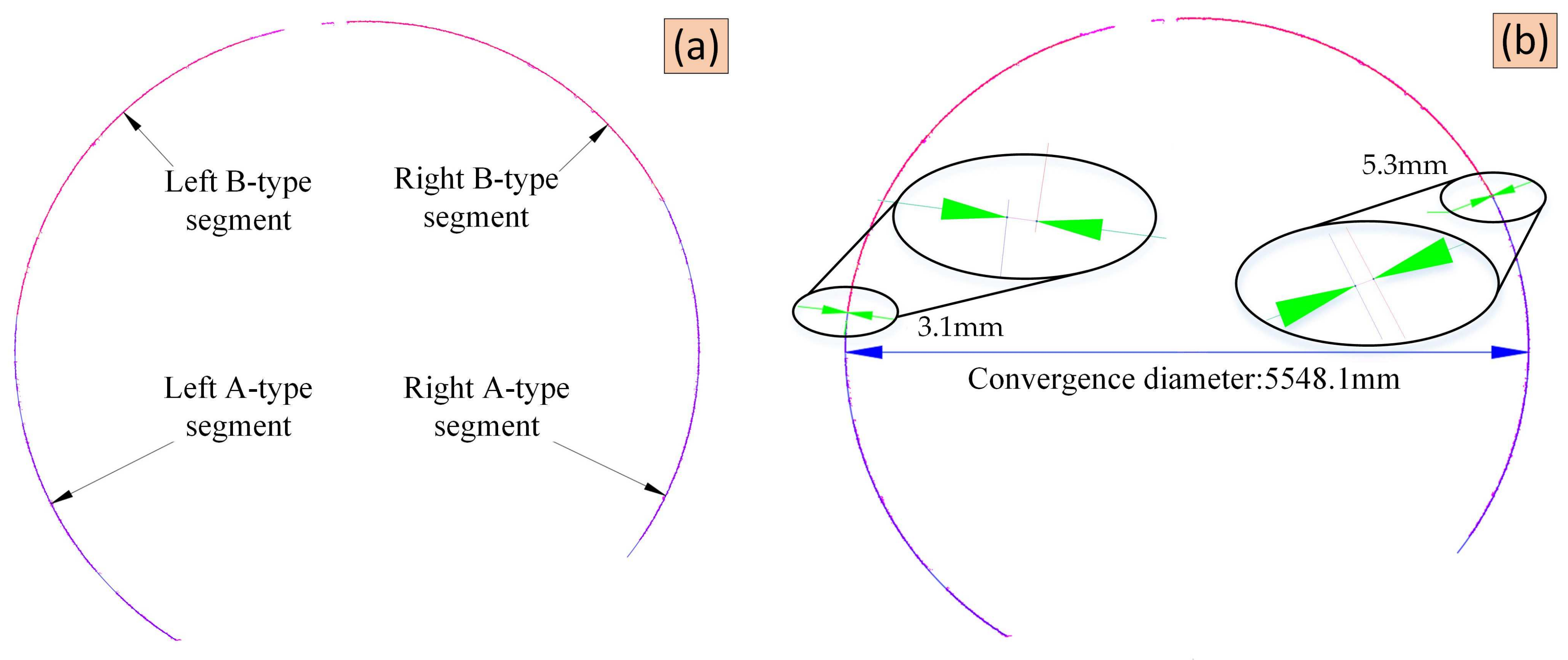
In addition to the convergence diameter, the method based on block fitting can complete the detection of radial dislocations. After the processing of steps (1) and (2), the obtained "clean" shield segment point clouds are fitted circle by circle. The maximum convergence iteration threshold and fitting precision are set. When the convergence conditions are fulfilled, the fitting circle parameters corresponding to the current segment point cloud, including the center and radius, are recorded. After the fitting converges and the correct circular parameters are obtained, the coordinates of the intersection points A and B between the radius line of the current tunnel section at the transverse seam and the fitting circle corresponding to the adjacent segment are calculated. The distance between AB is the radial offset value corresponding to the circular seam (Figure 11).
3. Results and Analysis
3.1. Study Area and SDMLS Data Generation
Experimental data were selected from the subway in Guangzhou, China, in operation since 2003. The foundation pit is planning to be excavated on the side of this test area, we used SDMLS to compare tunnel deformation before and after pit excavation. Before excavating the foundation pit, the SDMLS was used to detect the current state of the tunnel. In the foundation pit excavation process, a total station was used for automatic real-time monitoring. After the completion of foundation pit backfilling, the SDMLS was used to detect the tunnel again.
The experimental data were collected during non-operating hours (skylight time) at night, and the operation period was 3 h (00:00 to 03:00). The total station used five skylight times for manual measurement, and SDMLS used two skylight times. The length of the experimental line was 120 m, and the self-driven trolley ran at a normal and uniform speed of 2 km/h. The scanner model of Z + F PROFILER 9012 (range noise of 0.3 mm at 5 m and an angular accuracy of 8.48 arcsec) and Faro’s Focus350 (range noise of 0.2 mm at 5 m and an angular accuracy of 19 arcsec) were used for scanning. The Faro scanning frequency of the line was 220 Hz, and that of the point was 976 KHz. The number of scanning points in each section was more or less 4267, and the line spacing was approximately 3.7 mm. The laser point spacing at the waist segment on both sides of the tunnel was estimated as 1.8 mm. The parameter settings of the two types of scanners fulfilled the requirements of seam identification and convergence diameter detection.
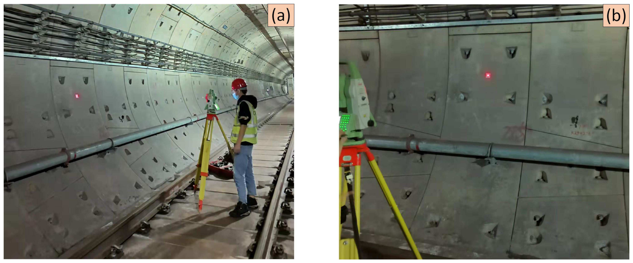
To determine the position of the middle point of the continuous seam between the standard block and the connecting block, this study used the following steps: 0.813 m was measured from the middle point of the continuous seam, and the intersection point on the standard block was marked as the convergence point. Next, to improve the measurement accuracy, the reflection plate was pasted at this position, and then the space distance between the center of the reflection plate was measured with the total station’s reflection plate measuring mode, plus the thickness of the reflection plate twice, as the convergence value of the tunnel diameter (Figure 12). The total station instrument used in this experiment was the Leica TS60 model, and the ranging accuracy of the reflector plate mode was 1 mm + 1 ppm, which can be used as the true value of this experiment.
3.2. Results
3.2.1. Result of Ring and Transverse Seams Detection
The ring seam and transverse seam were identified using the method described in Section 2.3. When ancillary facilities are installed at the waist of the tunnel, the transverse seam is blocked, and the transverse seam between the connecting block and the standard block can be calculated by the seam between the adjacent sealing block and the adjacent block, and the fitting parameters of the adjacent block. The ring seam and transverse seam are identified in Figure 13.
3.2.2. Result of Convergence Diameter Points Inspection
The method this study used for determining the position of the convergence diameter is consistent with that of manual inspection. This survey involved two methods of segment assembly: a continuous seam and a stagger seam. The convergence diameter endpoint for each assembly type was determined as follows:
- (1)
- Continuous Seam Points
Continuous seam assembly adopts a simple direct measurement method. A chord length of 813 mm is measured from A or A’ down at the middle of the seam aforementioned the two side diameters, which are positions B and B’ at one end of the convergence diameter, in Figure 14.
- (2)
- Stagger seam points
The stagger seam assembly is not consistent: the 1597 mm to point B is measured from the middle of the seam at A. Thus, the 539 mm to point B’ is measured from the middle of the seam at A’. Then, BB’ is the ideal position for the convergence diameter (Figure 14).
3.3. Accuracy Assessment
3.3.1. Absolute Accuracy Verification Based on the Total Station
The total station measuring method introduced in Section 3.1, which is taken as the true value of the convergence diameter, is used to obtain the convergence value of each ring segment diameter. The point cloud obtained by SDMLS scanning is divided into rings and segments using the method described in Section 2.3, and then the segment point cloud of each ring tube slice is obtained. The method described in Section 2.4 is used to fit the point cloud into a circle, and then the convergence diameter of the point cloud is calculated by the method described in Section 2.5. To maintain the position of convergence diameter obtained by the total station, the point cloud that is 0.02 m width in the middle of each ring tube is obtained and fitted. The difference between SDMLS and the total station is from −2.9 to 2.8 mm, the mean absolute deviation (MAD) is −0.2 mm, and the standard deviation (STD) is 1.5 mm (Figure 15). According to the specification, the convergence detection precision of the tunnel is ±3 mm, proving that the convergence diameter measured by SDMLS fulfills the specification. The systematic error causes mainly include the total station positioning error, scanner ranging error, and non-parallel error between the rail track and tunnel centerline.
3.3.2. Repeat Accuracy Verification for Round-trip Repeat Scan
To verify the stability of the SDMLS system and the reliability of the test results, this study repeated the experiment precision by using forward and backward scanning. Using the method described in Section 2, the convergence diameter test and the statistical deviation value of the convergence diameter were derived for the same tunnel. The range of the convergence diameter’s repeated difference is −1.9 to 2.0 mm, and the STD is 0.8 mm (Figure 16).
3.4. Accuracy Comparison of Different Scanners
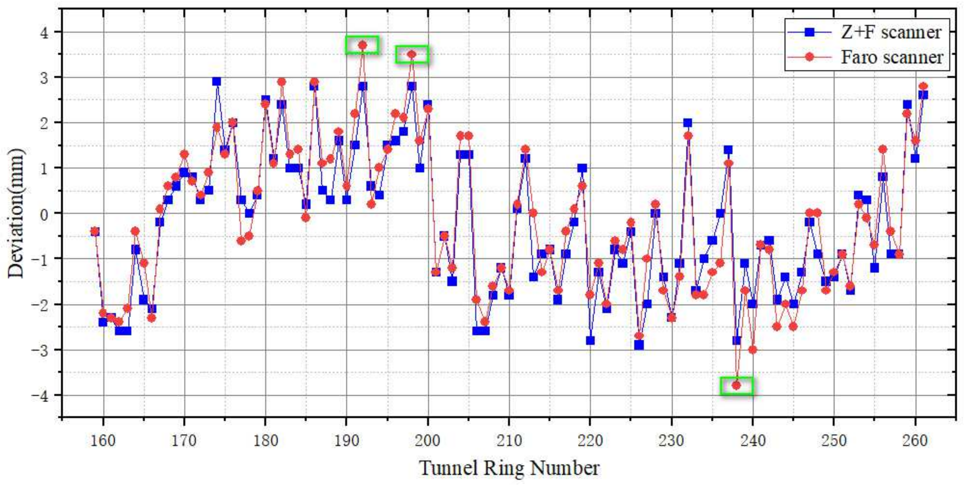
To verify the universality of the method proposed in this study, as described in Section 3.1, this study integrated Faro and Z + F laser scanning into the SDMLS system. The convergence diameters detected by the same segment were compared: the difference between the Faro scanner and Z + F scanner is from −1.2 to 1.3 mm, and the standard deviation is 0.5 mm (Figure 17).
The following conclusions were drawn: (1) This study presents a convergence diameter detection method based on SDMLS, which can be applied to different laser scanners. (2) The accuracy of the Faro scanner and Z + F scanner in detecting the convergence diameter is almost consistent. Some points of the convergence diameter detected by the Faro scanner were slightly larger than Z + F scanner (Figure 17). (3) Causes of the errors are described in Section 3.3.1.
3.5. Comparison of Ellipse Fitting and Block Fitting Results
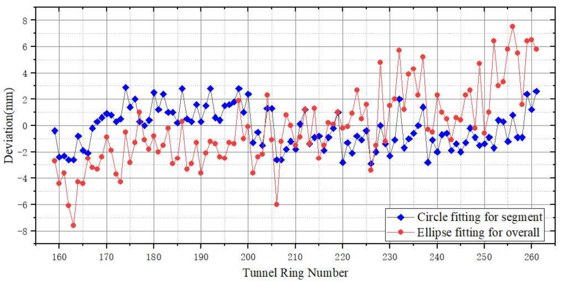
This part is based on Section 2.4 for the segment of the "clean" point cloud, and the fitting tunnel convergence diameter is based on the ellipse fitting method. The ellipse fitting results and test results of the proposed method were compared with the total station measurements. The ellipse fitting difference ranges from −7.6 to 7.5 mm, the MAD is −0.2 mm, and the STD is 3.0 mm. The difference between the method proposed in this study and the detection result of the total station is less than that of the elliptic fitting result (Figure 18).
4. Discussion and Future Works
The SDMLS has realized a uniform distribution of scan lines by scanning at a constant speed, which is conducive to seam extraction from 2D images. Compared with the direct use of the ellipse fitting measurement results, the accuracy of the block fitting method increased by 2 mm. This method can effectively solve the waist-area tunnel by eliminating missing data; thus, it is more applicable to engineering applications than ellipse fitting method. Engineering practice shows that differences in distinct areas of the tunnel environment affect the quality of the gray-level image. As a result, the generalization ability of the segment crack detection algorithm cannot achieve the desired level. At present, deep learning algorithms are used in experiments to fully automatically extract segment gaps. In the future, the author plans to continue to optimize and improve the algorithm.
5. Conclusions
On the basis of the MLS point cloud data, a block fitting method was proposed to detect the diameter convergence and radial dislocation of the shield tunnel. In the process of segment seam or/and positioning, a 3D point cloud rich in information is fully combined with the characteristics of clear 2D images by using a digital image processing algorithm. This approach efficiently extracts the characteristics of the seam and completes the mass point cloud data points ring and block. The optimal ellipse fitting method and iterative registration method are used to realize the initial filtering and fine denoising of the point cloud. The block fitting method is used to detect the convergence diameter with radial dislocations to effectively avoid model errors. The engineering application results show that the convergence diameter and radial dislocation detected by the method described in this study are consistent with those detected by the manual measurement method, and the standard deviation is better than 1 mm.
Author Contributions
Conceptualization, L.X.; methodology, L.X.; software, L.X.; validation, L.X.; formal analysis, L.X.; writing—original draft preparation, L.X., J.G. and J.N.; writing—review and editing, J.N., J.G., Y.Y., N.P. and Z.T.; visualization, L.X.; supervision, S.Z.; funding acquisition, L.X. and S.Z. All authors have read and agreed to the published version of the manuscript.
Funding
This work was financially supported by the Major Project of China Railway Design Corporation (No. 2021A240507), and the Science and Technology Planning Project of Tianjin Province (No. 20YFZCGX00710).
Data Availability Statement
Data and code from this research will be available upon request to the authors.
Acknowledgments
The authors sincerely thank the comments from anonymous reviewers and members of the editorial team.
Conflicts of Interest
The authors declare no conflict of interest.
References
- The Statistic and Analysis Report of Urban Rail Transit. 2020. Available online: https://www.camet.org.cn/tjxx/7647 (accessed on 9 April 2021).
- Li, Y.J.; Xu, H.; Zhang, Y.; Yao, J.J. Application of Carbon Fiber Cloth in Reinforcement of Metro Tunnel Disease. Appl. Mech. Mater. 2013, 353–356, 1525–1528. [Google Scholar] [CrossRef]
- Mukupa, W.; Roberts, G.W.; Hancock, C.M.; Al-Manasir, K. A review of the use of terrestrial laser scanning application for change detection and deformation monitoring of structures. Surv. Rev. 2016, 49, 116–199. [Google Scholar] [CrossRef]
- Feng, L.; Yi, X.; Zhu, D.; Xie, X.; Wang, Y. Damage detection of metro tunnel structure through transmissibility function and cross correlation analysis using local excitation and measurement. Mech. Syst. Signal Process. 2015, 60, 59–74. [Google Scholar] [CrossRef]
- Stiros, S.C.; Kontogianni, V. Mean deformation tensor and mean deformation ellipse of an excavated tunnel section. Int. J. Rock Mech. Min. Sci. 2009, 46, 1306–1314. [Google Scholar] [CrossRef]
- Xu, J.; Ding, L.; Luo, H.; Chen, E.J.; Wei, L. Near real-time circular tunnel shield segment assembly quality inspection using point cloud data: A case study. Tunn. Undergr. Space Technol. 2019, 91, 102998. [Google Scholar] [CrossRef]
- Du, L.; Zhong, R.; Sun, H.; Zhu, Q.; Zhang, Z. Study of the Integration of the CNU-TS-1 Mobile Tunnel Monitoring System. Sensors 2018, 18, 420. [Google Scholar] [CrossRef] [PubMed] [Green Version]
- Ao, X.; Wu, H.; Xu, Z.; Gao, Z. Damage Extraction of Metro Tunnel Surface from Roughness Map Generated by Point Cloud. In Proceedings of the 2018 26th International Conference on Geoinformatics, Kunming, China, 28–30 June 2018; pp. 1–4. [Google Scholar]
- Yang, B.; Fang, L. Automated Extraction of 3-D Railway Tracks from Mobile Laser Scanning Point Clouds. IEEE J. Sel. Top. Appl. Earth Obs. Remote Sens. 2014, 7, 4750–4761. [Google Scholar] [CrossRef]
- Stal, C.; De Wulf, A.; Nuttens, T. Tunnel measurements and point filtering: Automated point set filtering of cylindrical tunnel point sets. Gim Int. 2012, 26, 30–35. [Google Scholar]
- Wang, W.; Zhao, W.; Huang, L.; Vimarlund, V.; Wang, Z. Applications of terrestrial laser scanning for tunnels: A review. J. Traffic Transp. Eng. 2014, 1, 325–337. [Google Scholar] [CrossRef] [Green Version]
- Yan, L.; Liu, H.; Tan, J.; Li, Z.; Xie, H.; Chen, C. Scan Line Based Road Marking Extraction from Mobile LiDAR Point Cloud. Sensors 2016, 16, 903. [Google Scholar] [CrossRef]
- Huang, H.-W.; Cheng, W.-C.; Zhou, M.; Chen, J.; Zhao, S. Towards Automated 3D Inspection of Water Leakages in Shield Tunnel Linings Using Mobile Laser Scanning Data. Sensors 2020, 20, 6669. [Google Scholar] [CrossRef] [PubMed]
- Tan, K.; Cheng, X.; Ju, Q. Combining mobile terrestrial laser scanning geometric and radiometric data to eliminate accessories in circular metro tunnels. J. Appl. Remote Sens. 2016, 10, 030503. [Google Scholar] [CrossRef]
- Yue, Z.; Sun, H.; Zhong, R.; Du, L. Method for Tunnel Displacements Calculation Based on Mobile Tunnel Monitoring System. Sensors 2021, 21, 4407. [Google Scholar] [CrossRef] [PubMed]
- Zhang, H.; Xia, J. Research on convergence analysis method of metro tunnel section--Based on mobile 3D laser scanning technology. IOP Conf. Ser. Earth Environ. Sci. 2021, 669, 012008. [Google Scholar] [CrossRef]
- Cui, H.; Ren, X.; Mao, Q.; Hu, Q.; Wang, W. Shield subway tunnel deformation detection based on mobile laser scanning. Autom. Constr. 2019, 106, 102889. [Google Scholar] [CrossRef]
- Du, L.; Ruofei, Z.; Sun, H.; Wu, Q. Automatic monitoring of tunnel deformation based on high density point clouds data. ISPRS-Int. Arch. Photogramm. Remote Sens. Spat. Inf. Sci. 2017, 42, 353–360. [Google Scholar] [CrossRef] [Green Version]
- Walton, G.; Delaloye, D.; Diederichs, M.S. Development of an elliptical fitting algorithm to improve change detection capabilities with applications for deformation monitoring in circular tunnels and shafts. Tunn. Undergr. Space Technol. 2014, 43, 336–349. [Google Scholar] [CrossRef]
- Delaloye, D.; Diederichs, M.S.; Walton, G.; Hutchinson, J. Sensitivity Testing of the Newly Developed Elliptical Fitting Method for the Measurement of Convergence in Tunnels and Shafts. Rock Mech. Rock Eng. 2014, 48, 651–667. [Google Scholar] [CrossRef]
- Cao, Z.; Chen, D.; Peethambaran, J.; Zhang, Z.; Xia, S.; Zhang, L. Tunnel Reconstruction With Block Level Precision by Combining Data-Driven Segmentation and Model-Driven Assembly. IEEE Trans. Geosci. Remote Sens. 2021, 59, 8853–8872. [Google Scholar] [CrossRef]
- Sun, H.; Xu, Z.; Yao, L.; Zhong, R.; Du, L.; Wu, H. Tunnel Monitoring and Measuring System Using Mobile Laser Scanning: Design and Deployment. Remote. Sens. 2020, 12, 730. [Google Scholar] [CrossRef] [Green Version]
- Yu, A.; Mei, W.; Han, M. Deep learning based method of longitudinal dislocation detection for metro shield tunnel segment. Tunn. Undergr. Space Technol. 2021, 113, 103949. [Google Scholar] [CrossRef]
- Kang, Z.; Zhang, L.; Tuo, L.; Wang, B.; Chen, J. Continuous Extraction of Subway Tunnel Cross Sections Based on Terrestrial Point Clouds. Remote. Sens. 2014, 6, 857–879. [Google Scholar] [CrossRef] [Green Version]
- Dhal, K.G.; Das, A.; Ray, S.; Gálvez, J.; Das, S. Histogram Equalization Variants as Optimization Problems: A Review. Arch. Comput. Methods Eng. 2020, 28, 1471–1496. [Google Scholar] [CrossRef]
- Iqbal, B.; Iqbal, W.; Khan, N.; Mahmood, A.; Erradi, A. Canny edge detection and Hough transform for high resolution video streams using Hadoop and Spark. Clust. Comput. 2019, 23, 397–408. [Google Scholar] [CrossRef]
- Nguyen, T.T.; Pham, X.D.; Jeon, J.W. An improvement of the Standard Hough Transform to detect line segments. In Proceedings of the 2008 IEEE International Conference on Industrial Technology, Chengdu, China, 21–24 April 2008; pp. 1–6. [Google Scholar]
- Fujimoto, T.; Kawasaki, T.; Kitamura, K. Canny-Edge-Detection/Rankine-Hugoniot-conditions unified shock sensor for inviscid and viscous flows. J. Comput. Phys. 2019, 396, 264–279. [Google Scholar] [CrossRef]
- Cheng, Y.-J.; Qiu, W.; Lei, J. Automatic Extraction of Tunnel Lining Cross-Sections from Terrestrial Laser Scanning Point Clouds. Sensors 2016, 16, 1648. [Google Scholar] [CrossRef]
- Jia, D.; Zhang, W.; Liu, Y. Systematic Approach for Tunnel Deformation Monitoring with Terrestrial Laser Scanning. Remote Sens. 2021, 13, 3519. [Google Scholar] [CrossRef]
- Xu, X.; Yang, H.; Neumann, I. A feature extraction method for deformation analysis of large-scale composite structures based on TLS measurement. Compos. Struct. 2018, 184, 591–596. [Google Scholar] [CrossRef]
- Momen, A.; Johnson, B.K.; Chakhchoukh, Y. Parameters Estimation for Short Line Using the Least Trimmed Squares (LTS). In Proceedings of the 2019 IEEE Power & Energy Society Innovative Smart Grid Technologies Conference (ISGT), Washington, DC, USA, 18–21 February 2019; pp. 1–4. [Google Scholar]
- Alshqaq, S.S. On the least trimmed squares estimators for JS circular regression model. Kuwait J. Sci. 2021, 48, 1–13. [Google Scholar] [CrossRef]
- Ray, A.; Srivastava, D.C. Non-linear least squares ellipse fitting using the genetic algorithm with applications to strain analysis. J. Struct. Geol. 2008, 30, 1593–1602. [Google Scholar] [CrossRef]
- Borowski, L.; Banb, M. The Best Robust Estimation Method to Determine Local Surface. Balt. J. Mod. Comput. 2019, 7, 525–540. [Google Scholar] [CrossRef]
- Tan, Z.; Li, Z.; Tang, W.; Chen, X.-Y.; Duan, J. Research on Stress Characteristics of Segment Structure during the Construction of the Large-Diameter Shield Tunnel and Cross-Passage. Symmetry 2020, 12, 1246. [Google Scholar] [CrossRef]
- Dong, F.; Huang, J.; Li, A.; Gao, C. Analysis on Disease State of Urban Operational Subway Tunnels. Environ. Eng. 2021, 6, 54–62. [Google Scholar] [CrossRef]
Figure 1.
Flowchart of the method.

Figure 2.
SDMLS system: (a) hardware equipment; (b) operation mode; (c) 3D view of spiral; (d) top view of the spiral.
Figure 2.
SDMLS system: (a) hardware equipment; (b) operation mode; (c) 3D view of spiral; (d) top view of the spiral.

Figure 3.
Transverse seam error: (a) seam deviation; (b) seam position.

Figure 4.
Mapping relationship between point cloud and grayscale image of tunnel cross-section: (a) cylindrical projection model; (b) tiled projection plane.
Figure 4.
Mapping relationship between point cloud and grayscale image of tunnel cross-section: (a) cylindrical projection model; (b) tiled projection plane.

Figure 5.
Feature enhancement: (a) source image histogram; (b) source image; (c) equalization histogram; (d) equalization image.
Figure 5.
Feature enhancement: (a) source image histogram; (b) source image; (c) equalization histogram; (d) equalization image.

Figure 6.
Edge feature extraction: (a) longitudinal seams; (b) grayscale jump; (c) edge feature.

Figure 7.
Hough transform to extract vertical straight lines: (a) Hough transform detection results; (b) pixel statistics contained in the line; (c) initial longitudinal seam.
Figure 7.
Hough transform to extract vertical straight lines: (a) Hough transform detection results; (b) pixel statistics contained in the line; (c) initial longitudinal seam.

Figure 8.
Point cloud noise of cross-section: (a) noise (the blue part); (b) regional divisions.

Figure 9.
Point cloud filtering of tunnel section: (a) source point cloud; (b) ellipse fitting filtering; (c) model iterative filtering.
Figure 9.
Point cloud filtering of tunnel section: (a) source point cloud; (b) ellipse fitting filtering; (c) model iterative filtering.

Figure 10.
Local side view before (a) and after (b) point cloud denoising based on iterative closest point method.
Figure 10.
Local side view before (a) and after (b) point cloud denoising based on iterative closest point method.

Figure 11.
Radial dislocation detection by block fitting method: (a) segment segmentation; (b) convergence diameter and radial dislocation detection.
Figure 11.
Radial dislocation detection by block fitting method: (a) segment segmentation; (b) convergence diameter and radial dislocation detection.

Figure 12.
Manual method for tunnel convergence diameter measurement use total station (the red point represents the convergence point): (a) one convergence point is the left part of tunnel; (b) the other convergence point is the right part of the tunnel.
Figure 12.
Manual method for tunnel convergence diameter measurement use total station (the red point represents the convergence point): (a) one convergence point is the left part of tunnel; (b) the other convergence point is the right part of the tunnel.

Figure 13.
Result of ring seam and transverse seam: (a) the continuous seam; (b) the stagger seam.

Figure 14.
Two convergence diameter measurement methods: (a) endpoint marking for continuous seam; (b) endpoint marking for stagger seam.
Figure 14.
Two convergence diameter measurement methods: (a) endpoint marking for continuous seam; (b) endpoint marking for stagger seam.

Figure 15.
Comparison of convergence deviation between total station and SDMLS.

Figure 16.
Comparison of repeatability verification of forward and backward scanning base on SDMLS.

Figure 17.
Comparison of convergence deviation between total station and SDMLS (red is Z + F scanner, and blue is Faro scanner).
Figure 17.
Comparison of convergence deviation between total station and SDMLS (red is Z + F scanner, and blue is Faro scanner).

Figure 18.
Comparison of convergence deviation between ellipse fitting and the proposed method (red is the ellipse fitting method for overall tunnel points, and blue is the circle fitting method for block segment points).
Figure 18.
Comparison of convergence deviation between ellipse fitting and the proposed method (red is the ellipse fitting method for overall tunnel points, and blue is the circle fitting method for block segment points).

Publisher’s Note: MDPI stays neutral with regard to jurisdictional claims in published maps and institutional affiliations. |
© 2022 by the authors. Licensee MDPI, Basel, Switzerland. This article is an open access article distributed under the terms and conditions of the Creative Commons Attribution (CC BY) license (https://creativecommons.org/licenses/by/4.0/).
Share and Cite
MDPI and ACS Style
Xu, L.; Gong, J.; Na, J.; Yang, Y.; Tan, Z.; Pfeifer, N.; Zheng, S. Shield Tunnel Convergence Diameter Detection Based on Self-Driven Mobile Laser Scanning. Remote Sens. 2022, 14, 767. https://0-doi-org.brum.beds.ac.uk/10.3390/rs14030767
AMA Style
Xu L, Gong J, Na J, Yang Y, Tan Z, Pfeifer N, Zheng S. Shield Tunnel Convergence Diameter Detection Based on Self-Driven Mobile Laser Scanning. Remote Sensing. 2022; 14(3):767. https://0-doi-org.brum.beds.ac.uk/10.3390/rs14030767
Chicago/Turabian StyleXu, Lei, Jian Gong, Jiaming Na, Yuanwei Yang, Zhao Tan, Norbert Pfeifer, and Shunyi Zheng. 2022. "Shield Tunnel Convergence Diameter Detection Based on Self-Driven Mobile Laser Scanning" Remote Sensing 14, no. 3: 767. https://0-doi-org.brum.beds.ac.uk/10.3390/rs14030767
Note that from the first issue of 2016, this journal uses article numbers instead of page numbers. See further details here.