Snow Coverage Mapping by Learning from Sentinel-2 Satellite Multispectral Images via Machine Learning Algorithms

Abstract

Snow coverage mapping plays a vital role not only in studying hydrology and climatology, but also in investigating crop disease overwintering for smart agriculture management. This work investigates snow coverage mapping by learning from Sentinel-2 satellite multispectral images via machine-learning methods. To this end, the largest dataset for snow coverage mapping (to our best knowledge) with three typical classes (snow, cloud and background) is first collected and labeled via the semi-automatic classification plugin in QGIS. Then, both random forest-based conventional machine learning and U-Net-based deep learning are applied to the semantic segmentation challenge in this work. The effects of various input band combinations are also investigated so that the most suitable one can be identified. Experimental results show that (1) both conventional machine-learning and advanced deep-learning methods significantly outperform the existing rule-based Sen2Cor product for snow mapping; (2) U-Net generally outperforms the random forest since both spectral and spatial information is incorporated in U-Net via convolution operations; (3) the best spectral band combination for U-Net is B2, B11, B4 and B9. It is concluded that a U-Net-based deep-learning classifier with four informative spectral bands is suitable for snow coverage mapping.

1. Introduction

Remote sensing technology (e.g., satellite-based, unmanned aerial vehicle (UAV)-based, ground-based) can provide a nondestructive way of spatially and temporally monitoring the targets of interest remotely, which has drawn increasing attention recently with the rapid development of autonomous system innovation, sensing technology and image-processing algorithms, especially with convolutional neural network-based deep-learning approaches. Taking remote sensing in geosciences as an example, UAV multispectral images are used in [1] for bulk drag prediction of Riparian Arundo donax stands so that their impact on vegetated drainage channel can be assessed. Terrestrial laser scanning is also used in [2] to investigate physically based characterization of mixed floodplain vegetation. Meanwhile, the interest in agricultural applications of remote sensing technology has also been exponentially growing since 2013 [3], where the main applications of remote sensing in agriculture include phenotyping, land-use monitoring, crop yield forecasting, precision farming and the provision of ecosystem services [3,4,5,6].

Crop disease monitoring and, more importantly, the accurate early forecasting of crop disease outbreak by making use of the remote sensing data has also attracted much attention in recent years [6,7,8]. In particular, temperature and humidity are the two most important environmental factors determining the activities of pathogenic microorganisms. A good example is the wheat stripe rust, one of the most destructive diseases in wheat in China, whose outbreak potential is largely determined by temperature. On the one hand, snow covering in winter means freezing low temperature; however, a study has also shown that winter snow covering could also weaken the negative effects of extreme cold temperature on rust survival [9]. A crop disease outbreak forecasting model with the consideration of snow coverage and duration information would no doubt generate better prediction performance. However, it is still a challenge to obtain accurate snow coverage and duration data for use in a forecasting model [7]. This is because manually obtaining this information for various areas of interest (mountainous areas in particular) would pose serious logistics and safety issues for agronomists.

In recent decades, many remote sensing satellites with various sensors (including multispectral sensors) have been launched into Earth orbit, meaning that estimating snow coverage from satellite images turns out to be the most promising solution for large-scale applications. In particular, some of these satellite data are publicly accessible and completely free; for example, Sentinel-2 satellites can provide multispectral imagery with a 10-m resolution (the highest resolution among freely available satellites) and a 5-day global revisit frequency for spatial-temporal land surface monitoring [10]. One of the most challenging parts of snow coverage mapping via satellite imagery is to distinguish snow from cloud. The major issue is that snow and cloud share very similar appearance and color distribution, and, as a result, manually separating snow pixels from cloud pixels requires expert knowledge and is still a tedious and time-consuming process. This similarity (between snow and cloud) also poses challenges for image classification algorithms, particularly for color images.

Currently, there are several empirical threshold test-based tools available to classify snow and cloud, such as Fmask [11], ATCOR [12] and Sen2Cor [13]. Despite the great potential of accurate snow coverage mapping, there is surprisingly little literature directly focused on snow coverage segmentation via satellite images. In contrast, there is much more literature studying the segmentation of cloud and land-cover scenes [14,15,16,17]. Zhu and Woodcock reported an empirical threshold test-based method called Tmask that uses multi-temporal Landsat images to classify cloud, cloud shadow and snow, and they demonstrated that the multi-temporal mask method significantly outperformed the Fmask approach, which only uses single-date data in discriminating snow and cloud [18]. Zhan et al. reported a fully convolutional neural network to classify snow and cloud in pixel levels for Gaofen #1 satellite imagery, with an overall precision of 92.4% in their own dataset [19]. However, Gaofen #1 satellite imagery is unfortunately not publicly accessible, and their manually labeled dataset is not publicly available either. More often, within the snow classification-related studies, snow is only listed as one of the many sub-classes and accounts for very limited representation [16,20,21]. Although the empirical thresholds of test-based methods such as Fmask [11], ATCOR [12] and Sen2Cor [13] can provide rough snow prediction in most scenarios, studies that focused on improving snow coverage segmentation performance by making use of machine (deep)-learning algorithms are still missing. It should be highlighted that conventional machine-learning methods and recent deep-learning methods (in particular) have made significant breakthroughs with appreciable performance in various applications including agriculture, and these are therefore worth investigation for snow coverage mapping as well [22,23].

Therefore, in this study, we first carefully collected 40 Sentinel-2 satellite images with scenes including representative snow, cloud and background that are distributed across almost all continents. Each pixel of the 40 scenes is labeled into three classes—snow, cloud and background—via the semi-automatic classification plugin in QGIS; thus, they become the largest publicly available satellite imagery dataset dedicated to snow coverage mapping. We then compared the reflectance distributions of the three classes across the 12 Sentinel-2 spectral bands and found the most informative band combination that was able to distinguish snow, cloud and background. Lastly, we compared the classification performance of three representative algorithms—Sen2Cor for thresholds test-based method, random forest for traditional machine learning, and U-Net for deep learning. We showed that the U-Net model with the four informative bands (including B2, B11, B4 and B9) as inputs gave the best classification performance on our test dataset.

2. Materials and Methods

To make the work readable, the entire workflow is illustrated in Figure 1.

2.1. Satellite Image Collection

Sentinel-2 satellite images are freely accessible from several platforms, such as the Copernicus Open Access Hub [24], USGS EROS Archive [25] and Google Earth Engine [26] among others. In this study, all Sentinel-2 satellite images were directly downloaded from the Google Earth Engine via some basic scripts in Java. Our main purpose is to conduct snow mapping of Earth’s surface, therefore, we focused on the corrected Sentinel-2 Level-2A product instead of the Level-1C product, as the Level-2A provides Orthoimage Bottom Of Atmosphere (BOA) corrected reflectance products. Moreover, the Level-2A product has itself included a scene classification map, including cloud and snow probabilities at 60 m resolution, which are derived from the Sen2Cor algorithm. However, it should also be noted that Level-2A products are only available after December 2018, although a separate program is available to generate Level-2A products from Level-1C product.

There are a total of 12 spectral bands for Sentinel-2 Level-2A product, which include B1 (Aerosols), B2 (Blue), B3 (Green), B4 (Red), B5 (Red Edge 1), B6 (Red Edge 2), B7 (Red Edge 3), B8 (NIR), B8A (Red Edge 4), B9 (Water vapor), B11 (SWIR 1) and B12 (SWIR 2). The cirrus B10 is omitted as it does not contain surface information. Of the 12 available spectral bands, B2, B3, B4 and B8 are all at 10 m resolution, the resolutions of B5, B6, B7, B8A, B9 and B12 are 20 m, and the remaining two bands of B1 and B19 have 60 m resolution. Within all our downstream analyses, all spectral bands with resolutions different from 10 m were re-sampled to 10 m to achieve an equal spatial resolution across all spectral bands.

During our scene collection, we specifically choose scenes that include human- identifiable snow, cloud, or both snow and cloud. It is important to ensure that the snow and cloud scenarios are human identifiable, as we are doing a supervised machine-learning task and our next step data annotation is to label each pixel into three classes. To ensure that the collected dataset includes a large diversity of scenes (to be representative), we selected the scenes to cover different continents, years, months and land-cover classes. Lastly, we only kept a representative 1000 pixels × 1000 pixels region for each scene; this is, on the one hand, to reduce the redundant contents of a whole product and, on the other hand, to greatly reduce the amount of time needed for the following data annotation step.

2.2. Data Annotation

Upon downloading the representative images, the next step is to manually label them into different classes for machine/deep-learning model construction. The data annotation step involves manually labeling every pixel into one of three classes (i.e., snow, cloud and background) by human experts. As the multispectral satellite images are not readily human-readable, we first extract the B4, B3 and B2 bands and re-scale them into the three channels of a typical RGB image (i.e., false-color RGB image). However, it is obvious that snow and cloud share very similar colors (i.e., close to white) and texture across many scenes, thus it is almost impossible to distinguish them, especially when there are overlaps between snow and cloud. B12 (SWIR 2) is known to have a relatively better separation between snow and cloud than other bands, thus we also created a false-color image, with B2, B3 and B12 as the R, G, B channels, for each scene. Then, all the downstream labeling processes are performed on the false-color images.

The pixel-level labeling process was performed in QGIS platform (Version: 3.18.2) [27]. Recently, Luca Congedo developed a Semi-Automatic Classification Plugin for QGIS, which is reported to be able to ease and automate the phases of land-cover classification [28]. Therefore, our labeling processes were completed with the help of the Semi-Automatic Classification Plugin (Version: 7.9) [28]. Specifically, for each image, we first select and define several representative regions for each target class; then, we use the Minimum Distance algorithm of this plugin to group all other pixels into the pre-defined classes. All final generated classification masks were carefully checked by two human experts to make sure the label for snow and cloud is as correct as possible.

2.3. Sen2Cor Cloud Mask and Snow Mask

The Sentinel-2 Level-2A product itself includes a cloud confidence mask and snow confidence mask, which are both derived from the Sen2Cor system. The algorithm used by Sen2Cor to detect snow or cloud is based on a series of threshold tests that use top-of-atmosphere reflectance from the spectral bands as input; the thresholds are also applied on band ratios and several spectral indices, such as Normalized Difference Vegetation Index (NDVI) and Normalized Difference Snow Index (NDSI). In addition, a level of confidence is associated with each of these threshold tests, and the final output of the series of threshold tests are a probabilistic (0–100%) snow mask quality map and a cloud mask quality map [29]. In our study, the snow confidence mask and cloud confidence mask of each scene were directly downloaded from Google Earth Engine along with its Level-2A spectral band data. For a better visualization of the Sen2Cor classification performance, for each satellite scene, we put the cloud confidence mask, snow confidence mask and snow confidence mask into the three channels of a color image to generate the final Sen2Cor classification mask.

2.4. Random Forest with Bayesian Hyperparameter Optimization

The ‘sklearn.ensemble.RandomForestClassifier’ function in sklearn library (Version: 0.24.2) [30] in Python (Version: 3.8.0) is used to construct Random Forest (RF) models to evaluate the performance of traditional machine-learning algorithms in classifying snow and cloud with the inputs of independent BOA-corrected reluctance data from different spectral band combinations.

RF is a decision tree-based algorithm, which has been widely applied in crop disease detection [31]. To improve the prediction accuracy and control the problem of overfitting, we need to fine-tune several key hyper-parameters for the training of each RF model [32]. In this study, we mainly fine-tuned three hyper-parameters: the number of trees in the forest, the maximum depth of the tree and the minimum number of samples required to split an internal node. Instead of using random or grid search for the optimal hyperparameter combination, we applied the Bayesian Optimization [33] to find the optimal parameter combination for each RF model. Bayesian optimization enables finding out the optimal parameter combination in as few iterations as possible, which works by sequentially constructing a posterior distribution of functions (Gaussian process) that best describes the function you want to optimize. Here, we used the average of five-fold cross-validation scores, which resulted from training a random forest model with weighted F1 score as the loss function, as the optimization function of Bayesian optimization. After the Bayesian optimization, a random forest model with the optical parameters setting is trained.

We then applied both forward sequential feature selection (FSFS) and backward sequential feature selection (BSFS) to rank the importance of each spectral band and more importantly to find out the optimal band combination, which has fewer bands and at the same time can capture the most informative features. FSFS sequentially adds features and BSFS sequentially removes features to form a feature subset in a greedy fashion. FSFS starts with zero features; at each stage, it chooses the best feature to add based on the cross-validation score of an estimator (RF classifier in this study). By contrast, BSFS starts with full features and sequentially selects the least important features to be removed at each stage.

2.5. U-Net Training

U-Net is a convolutional network architecture for fast and precise segmentation of images [34], which has been applied for yellow rust disease mapping in [5,32]. In this study, U-Net is used as the representative deep-learning model for satellite image classification. It is noted that our collected satellite images are in the size of $1000\times 1000$ pixels. However, to make our deep-learning models rely less on large-size images and to greatly increase the samples size of training dataset, we set the model input to have a width of 256, and height of 256 and channels of N, where N depends on the used combination bands in different models. For each satellite image in the training dataset, we clipped it into small patches in a sliding window way—with a window size of $256\times 256$ pixels and a sliding step of 128 pixels. As a result, each satellite image will yield around 49 patches of size 256 × 256 × N.

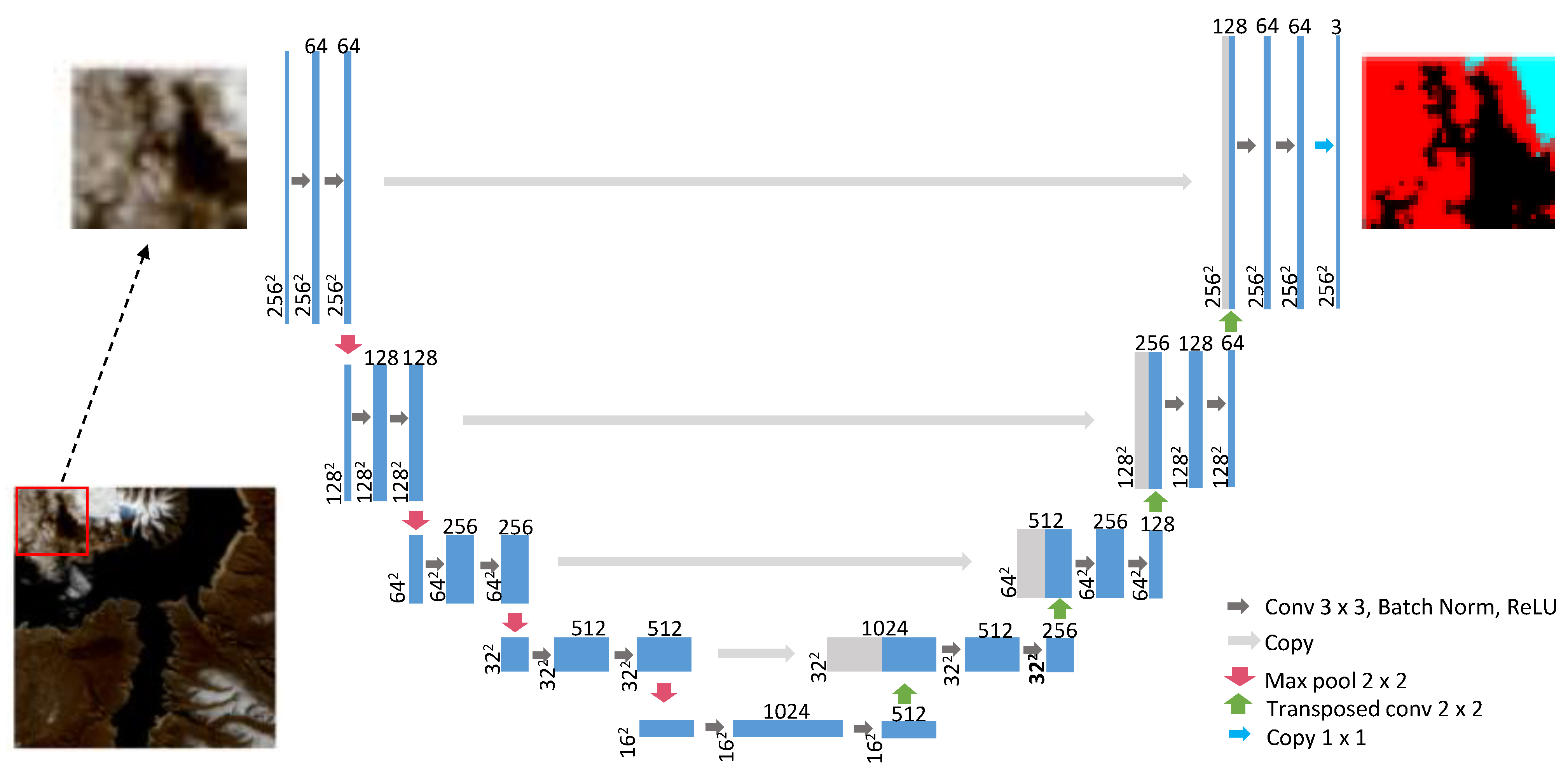
The details of the U-Net network architecture are shown in Figure 2. It consists of an encoding path (left side) and a decoding path (right side). Every block of the encoding path consists of two repeated $3\times 3$ unpadded convolutions, each followed by a batch normalization (BN) layer and a rectified linear unit (ReLU), then a $2\times 2$ max pooling operation with stride 2 is applied for downsampling. Each block of the decoding path includes a $2\times 2$ transpose convolution for feature upsampling, followed by a concatenation with the corresponding feature map from the encoding path, then two $3\times 3$ convolutions, each followed by a BN and a ReLU. The final layer is a $1\times 1$ convolution to map each pixel in the input to the desired number of classes.

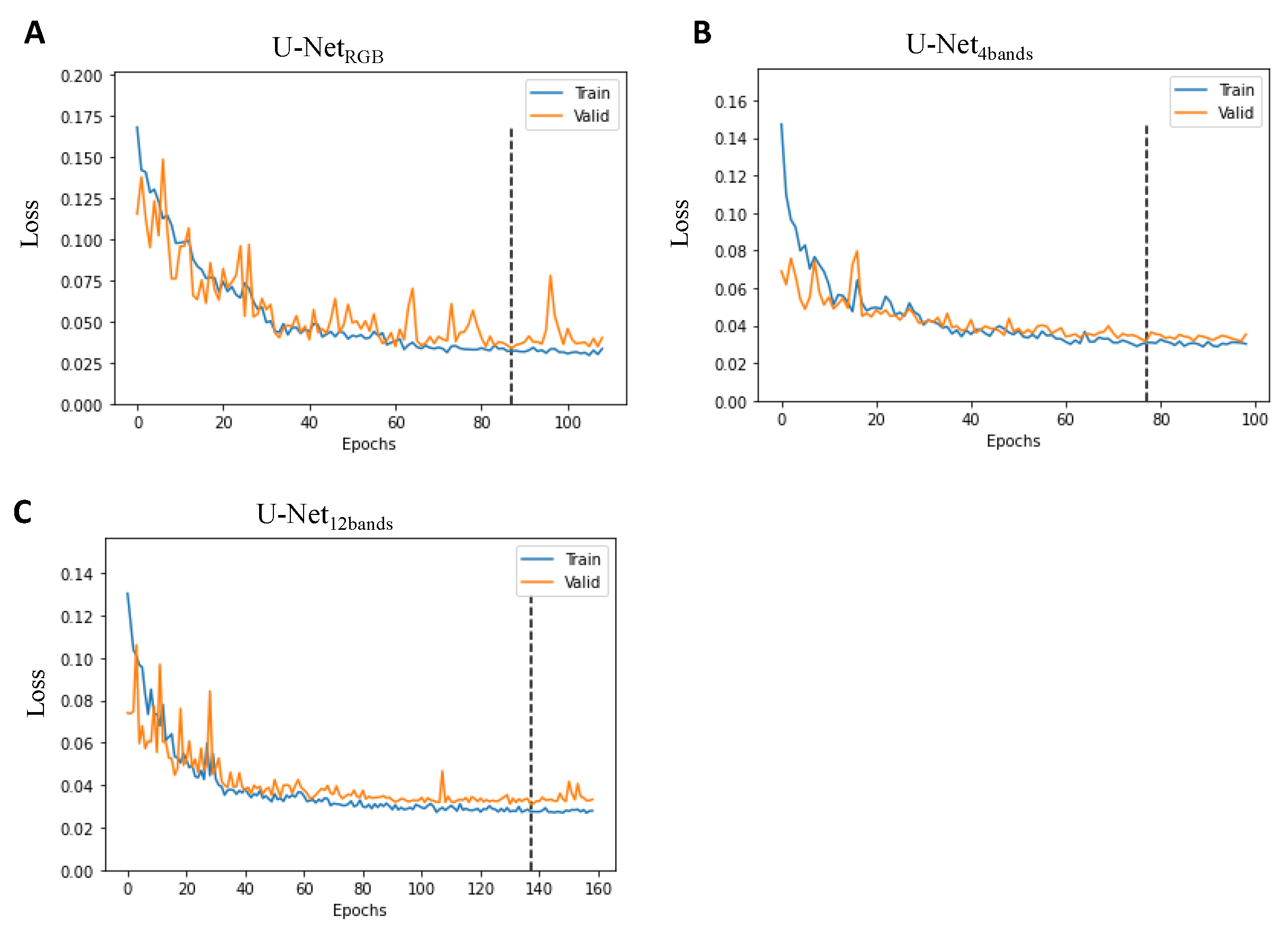
The U-Net model is constructed and trained based on the Pytorch deep leaning framework (Version: 1.7.1) [35]. For model training, we take the patches located in the first column or first row of the generated patch matrix of each training satellite image into the validation set and the remaining patches excluding those that have overlap with validation patches are selected as the training data, the ratio of the number of validation patches to training patches is about 19.1%. The model stops training until the loss of the validation data does not decrease after 20 epochs. To train the U-Net models, we used the weighted cross-entropy loss as the loss function, stochastic gradient descent as the optimizer with learning rate of 0.01 and momentum ratio of 0.9. The input batch size is set to be 4. The loss curves of the training processes for U-Net with different input bands are shown in Figure 3.

2.6. Evaluation Matrix

To systematically compare the classification performance of the different models, we have used the following evaluation matrices including prevision, recall, F1 score and Intersection Over Union(IoU) and Accuracy

$$\mathrm{Precision}=\frac{\mathrm{TP}}{\mathrm{TP}+\mathrm{FP}}$$

(1)

$$\mathrm{Recall}=\frac{\mathrm{TP}}{\mathrm{TP}+\mathrm{FN}}$$

(2)

$$\mathrm{F}1\_\mathrm{score}=2\times \frac{\mathrm{Precision}\times \mathrm{Recall}}{\mathrm{Precision}+\mathrm{Recal}}$$

(3)

$$\mathrm{Intersection}\mathrm{over}\mathrm{Union}\left(\mathrm{IoU}\right)=\frac{\mathrm{Area}\mathrm{of}\mathrm{Overlap}}{\mathrm{Area}\mathrm{of}\mathrm{Union}}$$

(4)

$$\mathrm{Accuracy}=\frac{\mathrm{TP}+\mathrm{TN}}{\mathrm{TP}+\mathrm{TN}+\mathrm{FP}+\mathrm{FN}}$$

(5)

where TP represents true positive numbers, FP represents false positive numbers and FN represents false negative numbers.

$$Loss\left(weightedcrossentropyloss\right)=-\sum _{c=1}^M{w}_c{y}_{o,c}log\left(p_{o,c}\right)$$

(6)

where $M=3$ is the number of classes (snow, cloud and background), $w_c$ is the weight value for class c which is defined as the ratio between the total number of pixels in the training set and the number of pixels in class c, $y_{o,c}$ is binary indicator (0 or 1) if class label c is the correct classification for observation o, $y_{o,c}$ is the predicted probability of observation o is of class c.

3. Results

3.1. Largest Snow-Mapping Satellite Image Dataset

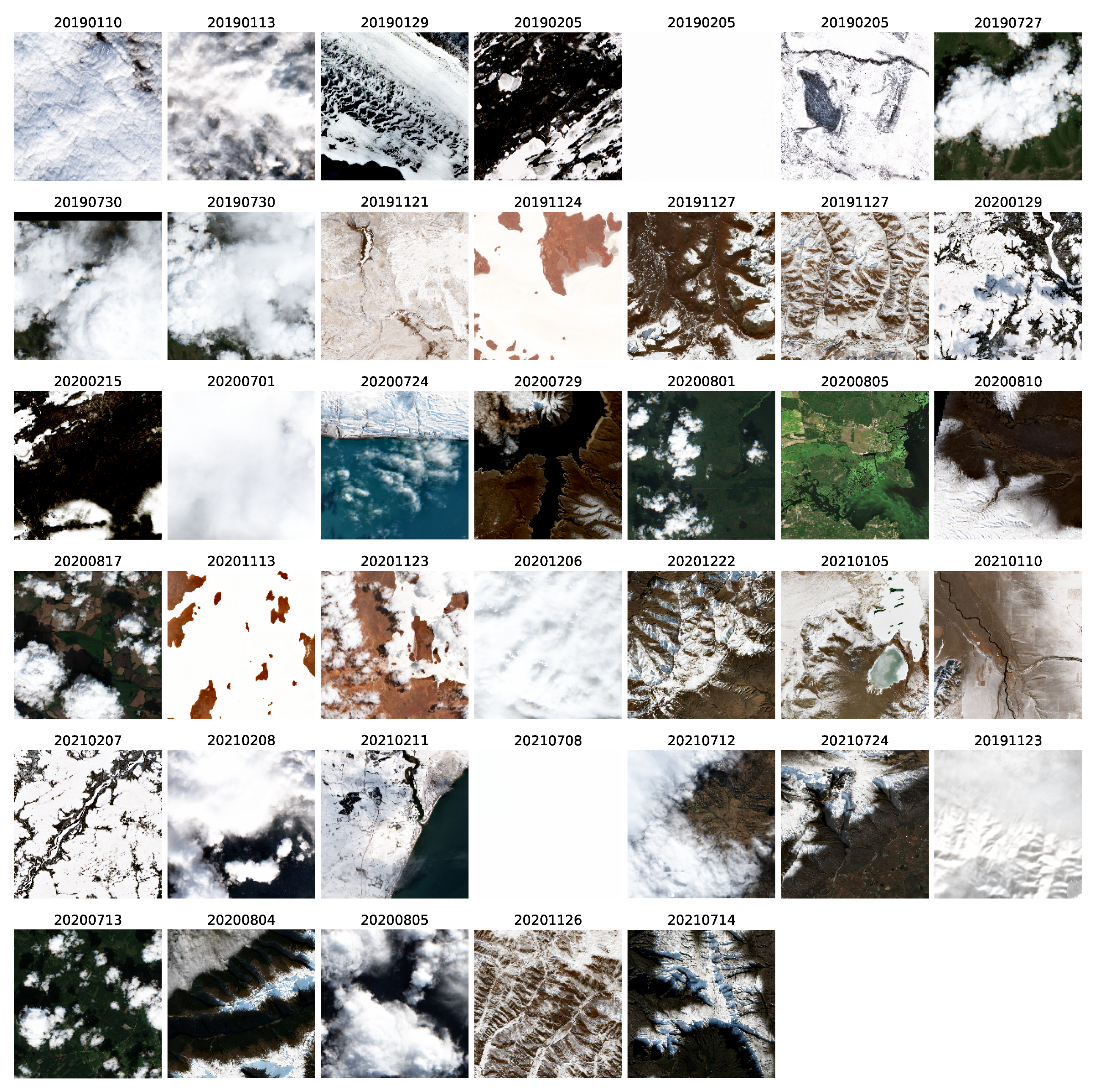
To validate and compare different methods in classifying snow and cloud for satellite images, we carefully searched and selected 40 Sentinel-2 L2A scenes across the globe as displayed in Figure 4. In addition, the details about their product ID, coordinates and timing are listed in

Table 1. Product IDs and coordinates of the 40 collected scenes.

Product ID	X Coordinate	Y Coordinate	Date
20190110T112439_20190110T112436_T30UVG	−2.96	55.25	10 January 2019
20190113T113429_20190113T113432_T30UVG	−4.09	55.17	13 January 2019
20190129T151649_20190129T151651_T20UNA	−62.2	50.16	29 January 2019
20190205T055031_20190205T055025_T45VUE	85.08	57.71	5 February 2019
20190205T164459_20190205T164614_T17ULA	−82.53	54.86	5 February 2019
20190205T164459_20190205T164614_T17ULA	−83.13	54.47	5 February 2019
20190727T035549_20190727T040012_T47SPT	100.5	33.99	27 July 2019
20190730T040549_20190730T041756_T47SMS	98.79	33.4	30 July 2019
20190730T040549_20190730T041756_T47SMT	98.77	33.68	30 July 2019
20191121T062151_20191121T062148_T42UWV	69.8	48.97	21 November 2019
20191124T005709_20191124T010446_T53HNE	136.05	−31.79	24 November 2019
20191127T041109_20191127T041653_T47SMS	98.95	33.38	27 November 2019
20191127T041109_20191127T041653_T47SPT	100.16	34.18	27 November 2019
20200129T151641_20200129T151643_T20UNA	−61.71	50.32	29 January 2020
20200215T054929_20200215T054925_T45VUE	84.81	57.94	15 February 2020
20200701T095031_20200701T095034_T34VFN	24.22	60.46	1 July 2020
20200724T142739_20200724T143750_T18FXK	−72.5	−50.18	24 July 2020
20200729T142741_20200729T143445_T19GCR	−70.2	−40.51	29 July 2020
20200801T182919_20200801T183807_T12VWH	−110.14	56.28	1 August 2020
20200805T085601_20200805T085807_T35UQS	30.37	51.06	5 August 20205
20200810T141739_20200810T142950_T19GCP	−70.8	−42.4	10 August 2020
20200817T084559_20200817T085235_T36UXD	35.63	52.73	17 August 2020
20201113T005711_20201113T005712_T53JNF	135.86	−31.65	13 November 2020
20201123T005711_20201123T010434_T53HNE	135.79	−31.71	23 November 2020
20201206T041141_20201206T041138_T47SNT	99.74	33.72	6 December 2020
20201222T111501_20201222T111456_T29RPQ	−7.74	31.1	22 December 2020
20210105T050209_20210105T050811_T45SUR	85.74	32.43	5 January 2021
20210110T182731_20210110T182953_T12TVR	−111.66	45.12	10 January 2021
20210207T151649_20210207T151817_T20UNA	−62.05	50.29	7 February 2021
20210208T112129_20210208T112318_T30VWJ	−1.57	57.14	8 February 2021
20210211T113319_20210211T113447_T30VWJ	−2.02	57.31	11 February 2021
20210708T141051_20210708T142222_T20HLB	−64.31	−39.38	8 July 2021
20210712T082611_20210712T084900_T34JBM	18.11	−30.39	12 July 2021
20210724T081609_20210724T083856_T34HCJ	19.67	−33.41	24 July 2021
20191123T111259_20191123T112151_T29RNQ	−8.3	31.22	23 November 2019
20200713T103031_20200713T103026_T33VWH	15.31	60.46	13 July 2020
20200804T223709_20200804T223712_T59GLM	169.47	−44.02	4 August 2020
20200805T001109_20200805T001647_T55GCN	145.04	−42.94	5 August 2020
20201126T041121_20201126T041842_T47SNT	100.09	33.93	26 November 2020
20210714T081609_20210714T083805_T34HCJ	19.16	−33.13	14 July 2021

.

The 40 sites have been chosen to ensure scene diversity. In particular, the 40 sites are distributed across all six continents except for Antarctica. With the constant high temperature in the low latitudes, our selected snow and cloud scenes are all distributed in middle- and high-latitude areas. Since the Sentinel-2 Level-2A products have only been available since December 2018, our collected scenes are all dated from the last three years, i.e., 2019, 2020 and 2021. For each scene, all 12 atmospheric corrected spectral bands, i.e., B1, B2, B3, B4, B5, B6, B7, B8, B8A, B9, B11 and B12, are collected, and the cloud confidence mask and the snow confidence mask which are derived from the Sen2Cor algorithm are also downloaded along with the spectral bands by the Google Earth Engine. Each band of the scene is re-sampled to 10 m resolution. For each scene product, we only kept a representative region, where the sizes of width and height are both 1000 pixels, which contains human identifiable snow or cloud.

Every pixel of all 40 collected satellite images were labeled into three classes including snow, cloud and background using the Semi-Automatic Classification Plugin [28] in QGIS. We took six representative scenes as the test dataset, and their false-color RGB images and classification masks are shown in Figure 12. The remaining 34 scenes were put into the training dataset, and their RGB images and classification masks are shown in Figure 5 and Figure 6, respectively.

3.2. Spectral Band Comparison

Snow and cloud are both white bright objects seen from the satellite RGB images, and they are often indistinguishable in most scenarios by only looking at RGB images. We first compared the reflectance distributions of snow, cloud and background in the 12 spectral bands from the Sentinel-2 L2A product. From the boxplots in Figure 7, we could first observe that the background pixels have relative low reflectance values across all 12 spectral bands, and the median reflectance values are all less than 2500. Snow and cloud showed similar and relatively high reflectance values (median reflectance values are greater than 5000) in the first ten spectral bands; however, they also both have high reflectance variations in these ten bands.

Regarding snow and cloud, B12 and B11 are the top two bands that best separate snow and cloud, with a median reflectance around 950 in snow, compared to that of around 2500 in the cloud. This is in line with our expectations, as B12 and B11 are both designed to measure short-wave infrared (SWIR) wavelengths, and they are often used to differentiate between snow and cloud. However, the distribution of background is very similar to snow in B11 and B12 although with larger fluctuations. B9, B1 and B2 are the three next bands that have a relatively larger distribution difference between snow and cloud. Interestingly, even though snow and cloud have very similar reflectance distributions in the first 10 bands, the cloud has a slightly higher median value than snow in nine out of the ten bands (except B4). In summary, there are several spectral bands that have good separation between any two of the three classes; however, there is no single band that clearly separates the three classes simultaneously.

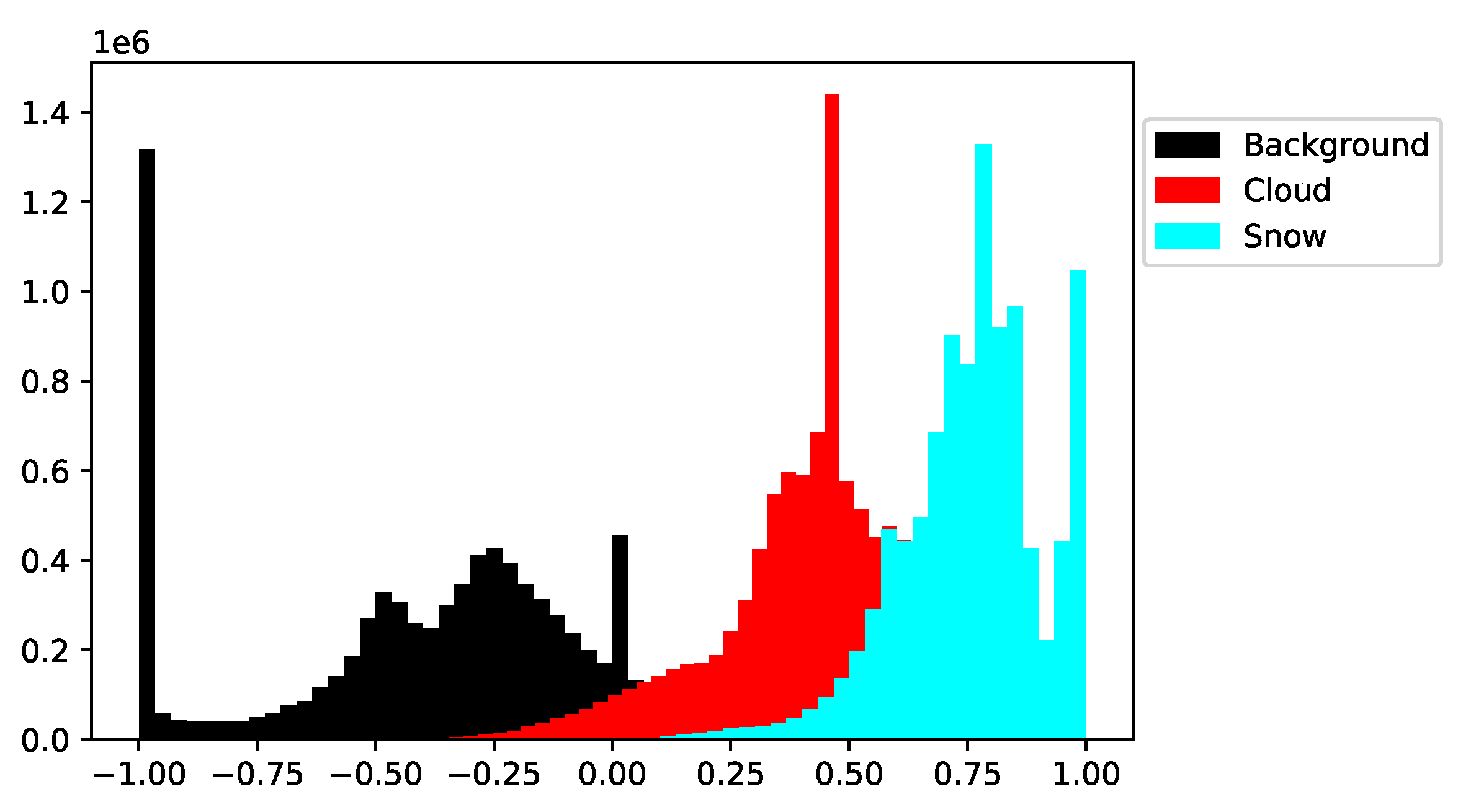
The Normalized Difference Snow Index (NDSI) has been suggested to be useful in estimating fractional snow cover [36,37]. It measures the relative magnitude of the reflectance difference between the visible green band and SWIR band. Here we also compared the NDSI distribution of snow, cloud and background in the training dataset, where the results are displayed in Figure 8. Our results showed that despite there being three major different spikes representing the three classes respectively, the huge overlaps between the snow spike and the cloud suggest that NDSI (though being the best index for snow mapping) is not a very accurate index to distinguish snow and cloud.

3.3. Optimal Band Combination

Our results in the previous section have demonstrated that no single spectral band (or index) is able to give clean separations between the three classes, i.e., snow, cloud and background. However, combining several bands is very promising. For example, the background pixels have clear separations with snow and cloud across the first ten bands, and the reflectance distribution of cloud is largely different from that in background and the snow within B12 or B11. Among the 12 spectral bands of the Sentinel-2 Level-2A product, some bands may capture similar features and thus may be redundant when used to distinguish the three classes. To find out the optimal band combination that captures the most useful information to discriminate the three classes that at the same time has fewer (saving computation resources) bands included, we applied both Forward Sequential Feature Selection (FSFS) and Backward Sequential Feature Selection (BSFS) (please refer to the Methods section for details), where their results are displayed in Figure 9.

As shown in Figure 9, the B2 (Blue) band is ranked as the most important band by both forward and backward sequential feature selection. B12 and B11 are two SWIR bands, and they are listed as the second most important bands by FSFS and BSFS, respectively. However, the band combination of B2 and B12 slightly outperforms the B2 and B11 combination when used as an input for constructing models to separate the three classes (OOB errors 0.109 vs. 0.123). FSFS and BSFS both identified B4 (Red) as the third most important band, and again the combination of B2, B11 and B4 identified by BSFS demonstrated as the best three-band combination. The sequential addition of more bands into the model input subset gives minimal improvements, especially when the top four bands have already been included. As a result, we take the combination of B2, B11, B4 and B9 as the most informative band set of Sentinel-2 Level-2A products for separating snow, cloud and background. It should be noted, although we re-sampled each band to the highest 10 meter resolution, the original resolutions for B2 and B4 are 10 m, B11 is 20 m and B9 is 60 m.

3.4. Performance Comparison for RF Models with Various Band Combinations

We trained three RF models, each with a different band combination as input, and compared their performance in classifying snow, cloud and background. The three-band combinations are RGB bands (B4, B3 and B2), the informative four bands (B2, B11, B4 and B9) and all 12 bands (B1, B2, B3, B4, B5, B6, B7, B8, B8A, B9, B11 and B12). The hyper-parameters of each random forest model were optimized independently by Bayesian optimization to achieve each model’s best performance.

The comparison of four evaluation scores (precision, F1 score, recall and IoU) between the three RF models is demonstrated in Figure 10 (on the training dataset) and Figure 11 (on the test dataset). The three RF models showed very close and good performance (all above 0.86) in predicting background pixels across all four evaluation scores. This is in line with our previous observation that background pixels have distinct BOA reflectance distribution compared to cloud and snow in each of the first ten bands (Figure 7). The most apparent difference between the three models is that the RF model trained on RGB bands (RF${}_{RGB}$) exhibited very poor performance in predicting both cloud and snow. For example, the IoU of RF${}_{RGB}$ in predicting cloud and snow are both below 0.35, and F1 scores are both only around 0.5. These results demonstrate the RGB bands (i.e., B4, B3 and B2) do not contain enough information to discriminate snow from cloud. This finding is also reflected by the fact that snow and cloud share similar reflectance distribution patterns across the three bands.

The RF model trained on the four informative bands (RF${}_{4bands}$) and the RF model trained on all 12 bands (RF${}_{12bands}$) exhibited very close performance in predicting all three classes, and they both significantly outperform the RF${}_{RGB}$ model in predicting both cloud and snow. The four bands input (B2, B11, B4 and B9) for RF${}_{4bands}$ was selected by BSFS to maximize the informative features and simultaneously minimize the number of bands. The previous section (Figure 9) has demonstrated that the top 4 important bands combined accounted for almost all the informative features in classifying the three classes. This explains why RF${}_{4bands}$ and RF${}_{12bands}$ showed close performance and are much better than RF${}_{RGB}$. A striking finding is that RF${}_{4bands}$ is even marginally better than RF${}_{12bands}$ in classifying the three classes based on all four evaluation scores, except for the precision of cloud and recall of snow. This may be due to the fact that the inclusion of more similar or non-relevant bands may make the machine-learning model at higher risk of overfitting on the training dataset, and this point is supported by the finding that RF${}_{12bands}$ slightly outperformed RF${}_{4bands}$ in classifying all three classes across the four evaluation scores in the training dataset (please refer to Figure 10).

3.5. Performance Comparison for U-Net with Various Band Combinations

In addition to the RF models, we also trained three U-Net models with RGB bands, informative four bands and all 12 bands as inputs. Except for the input layer, all other layers of the U-Net structure are the same for the three U-Net models. We then compared their classification performance based on the four evaluation metrics.

Similar to the RF models, the three U-Net models achieved close and good performance (all above 0.84) in classifying background pixels according to all four evaluation scores. The U-Net model with informative four bands as inputs (U-Net${}_{4bands}$) and the U-Net model with all bands as inputs (U-Net${}_{12bands}$ model) also exhibited close performance in predicting snow pixels and cloud pixels according to the four scores, even though the U-Net${}_{4bands}$ model slightly and consistently outperformed the U-Net${}_{12bands}$ model. The U-Net model with RGB bands as inputs (U-Net${}_{RGB}$) apparently fell behind U-Net${}_{4bands}$ and U-Net${}_{12bands}$ in classifying snow and cloud in almost all evaluation scores, except that the three models all achieved nearly perfect scores (all are greater than 0.987) on precision for cloud.

3.6. Comparison between Sen2Cor, RF and U-Net Models

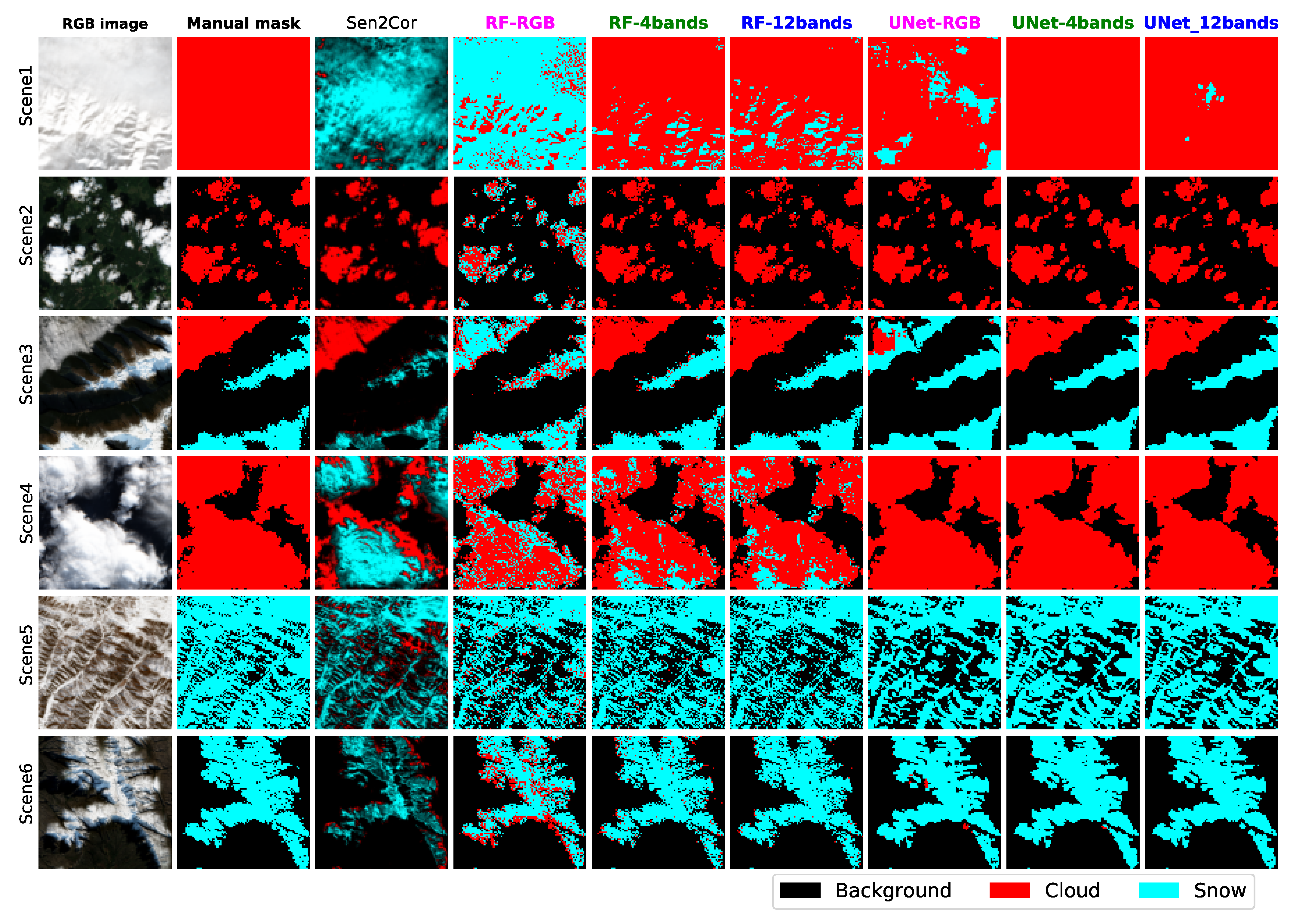
We then compared the classification performance of Sen2Cor, RF and U-Net models. In terms of overall accuracy, Sen2Cor gave very poor classification results (only 58.06%) on our selected six test scenes, apparently falling far behind other models (

Table 2. Overall accuracy of different models.

Overall Accuracy (%)	Sen2Cor	RF	U-Net
RGB	-	69.06%	87.72%
Informative 4 bands	-	90.03%	93.89%
All 12 bands	58.06%	89.65%	93.21%

). The poor classification performance of Sen2Cor is also reflected in its generated classification masks, which are listed in the third column of Figure 12. The Sen2Cor misclassified almost all cloud pixels in the first scene and most cloud pixels in the third scene into snow pixels; it also misclassified many snow pixels, which are mainly located at the boundaries between snow and background, in the last two scenes into clouds.

The three U-Net models all clearly outperformed their corresponding RF models. The greatest improvement came from the comparison between RF${}_{RGB}$ and U-Net${}_{RGB}$. The overall accuracy for RF${}_{RGB}$ is 69.06%, while it significantly increased to 87.72% using U-Net${}_{RGB}$ which is even closer to the performance of RF${}_{12bands}$ (89.65%). As with Sen2Cor, RF${}_{RGB}$ misclassified almost all cloud pixels in the first scene into snow; however, U-Net${}_{RGB}$ managed to correctly classify around 80% of the cloud pixels in the first scene. Both RF${}_{RGB}$ and U-Net${}_{RGB}$ tend to predict all snow and cloud pixels in the third scene as snow pixels. Furthermore, RF${}_{RGB}$ misclassified a lot of cloud pixels in the second scene and the fourth scene into snow and predicted many snow pixels in the last scene as cloud pixels, while U-Net${}_{RGB}$ does not have such issues (Figure 12). The above results indicate that the pure pixel-level reflectance from the RGB bands does not contain enough informative features to discriminate snow from cloud; the additional addition of spatial information as employed by U-Net model greatly improved the classification results.

Even though the overall accuracy of RF${}_{4bands}$ and RF${}_{12bands}$ reached around 90%, which is a huge improvement over RF${}_{RGB}$, they still both misclassified many cloud pixels into snow in the first and fourth scene. U-Net${}_{4bands}$ and U-Net${}_{12bands}$ further increased the overall accuracy to above 93%, and with U-Net${}_{RGB}$ they all avoided such “cloud to snow”misclassification issues in the fourth scene, U-Net${}_{4bands}$ even further uniquely correctly classified all cloud pixels in the first scene (Figure 12). U-Net${}_{4bands}$ achieved the highest overall accuracy of 93.89%, and this, combined with its outstanding score in the other four evaluation matrices (Figure 11), makes it the best model among the six models we have studied to do snow mapping for Sentinel-2 imagery.

4. Discussion

Snow coverage information is important for a wide range of applications. In agriculture, in particular, accurate snow mapping could be a vital factor for developing models to predict future disease development. However, accurate snow mapping from satellite images is still a challenging task, as cloud and snow share similar spectral reflectance distribution (visible spectral bands in particular), and therefore they are not easily distinguishable. To our best knowledge, there is no large annotated satellite image dataset especially for the task of snow mapping that is currently publicly available. Although Hollstein et al. [16] manually labeled dozens of small polygonal regions from scenes of Sentinel-2 Level-1C products across the globe at 20 m resolution, the small isolated irregular polygons are not useful enough to train convolutional neural network-based models. Baetens et al. [20] annotated 32 scenes of Sentinel-2 Level-2A products in 10 locations at 60 m resolution; however, they were mainly focused on generating cloud masks, and snow has very limited representation. As a result, we carefully collected and labeled 40 scenes of Sentinel-2 Level-2A products at the highest 10 m resolution, which includes a wide representative of snow, cloud and background landscape across the globe. The proposed database would on the one hand be used to evaluate the performance of different snow prediction tools, and on the other hand enable the future development of more advanced algorithms for snow coverage mapping.

Threshold tests-based tools (such as Sen2Cor) could be used to make fast and rough estimations of snow or cloud. However, our results have demonstrated that they can be misleading under some circumstances. In particular, Sen2Cor tends to mis-classify the cloud under a near-freezing environment temperature into snow, such as the case in the first and fourth scene of the test dataset (Figure 7). The thin layer of snow located in the junction between snow and background are also often misclassified to be cloud. Thus, accurate snow coverage mapping requires much better snow and cloud classification tools.

The Sentinel-2 Level-2A product includes 12 BOA-corrected reflectance bands. Our results show that no single band can provide clean separations between snow, cloud and background; each of the 12 bands may contain redundant or unique features that are useful to classify the three classes. Including too many features, such as including all 12 bands, may easily lead to overfitting on training data for most machine-learning and deep-learning algorithms, especially when the training dataset is not large enough. Thus, identifying the optimal band combination that contains most of the informative features while also containing a few bands is essential. Our forward feature selection and backward feature selection both agreed B2 (blue) is the most important band to separate the three classes. The combination of B2, B11, B4 and B9 reserves almost all informative features among all 12 bands for separating the three classes. Therefore, our results provide guidance for selecting bands for the following studies aimed at developing better snow-mapping tools.

Random Forest as the representative traditional machine-learning algorithm provides much better classification performance than the threshold test-based method Sen2Cor, especially when feeding the RF model with the four informative bands or all 12 bands. However, all three RF models have the issue of “salt-and-pepper” noise on their classification masks [32]. This issue does not only reflect the high variance of spectral reluctance values of each band within the three classes but also reflects the limitations of the traditional machine-learning algorithms. Traditional machine-learning algorithms, such as RF, only use pixel-level information, i.e., the reflectance values of each band for the same pixel, to make class predictions. They failed to make use of the information from the surrounding pixels or the broad spatial information. In contrast, the convolutional neural network-based deep-learning models such as U-Net exploit the surrounding pixel information by convolution operations and take advantage of the broad spatial information by repeated convolution and pooling operations. Therefore, the U-Net models all bypass the “salt-and-pepper” issue and give even better classification performance than the RF models.

The important role of spatial information in distinguishing snow and cloud is further highlighted when comparing classification performance between U-Net${}_{RGB}$ and RF${}_{RGB}$. The large overlaps of the reflectance distribution of the RGB bands between snow and cloud and the poor classification performance of RF${}_{RGB}$ demonstrate that pixel-level information of only RGB bands contains very limited features that can be used to separate the three classes. In contrast, U-Net${}_{RGB}$, also only fed by RGB bands but incorporating spatial information by the neural networks, can achieve significant improvements in classification performance compared to RF${}_{RGB}$. This raises an interesting open question for future studies, i.e., with a larger training dataset and improved neural network algorithms, is it possible to build satisfactory models with inputs of only RGB bands?

In terms of practical applications, although we have demonstrated that the U-Net model fed with the four informative bands (RF${}_{4bands}$) achieved the best prediction performance in our test dataset, and is much better than Sen2Cor and RF models, we should acknowledge that the efficient execution of deep-learning models often requires advanced hardware (e.g., GPU) and higher computation demands, thus making it less convenient to implement than the threshold test-based methods. However, with technology development and algorithm evolution, the application of deep-learning models in satellite images will become mainstream in the future.

5. Conclusions and Future Work

This work investigates the problem of snow coverage mapping by learning from Sentinel-2 multispectral satellite images via conventional machine- and recent deep-learning methods. To this end, the largest (to our best knowledge) satellite image dataset for snow coverage mapping is first collected by downloading Sentinel-2 satellite images at different locations and times, followed by manual data labeling via a semi-automatic data labeling tool in QGIS. Then, both a random forest-based conventional machine-learning approach and a U-Net-based deep-learning approach are applied to the labeled dataset so that their performance can be compared. In addition, different band inputs are also compared including a RGB three-band image, selected four bands via feature selection, and full multispectral bands. It is shown that (1) both conventional machine-learning and recent deep-learning methods significantly outperform the existing rule-based Sen2Cor product for snow mapping; (2) U-Net generally outperforms the random forest since both spectral and spatial information is incorporated in U-Net; (3) the best spectral band combination for snow coverage mapping is B2, B11, B4 and B9, even outperforming all spectral band combinations.

Although the results in this study are very encouraging, there is still much room for further development. For example, (1) in terms of data source, more labeled images from different locations and under diverse background conditions are required to generate a more representative dataset; (2) in terms of algorithm, the representative machine-learning algorithm (e.g., random forest, U-Net) are compared to obtain a baseline performance in this study, and more advanced deep-learning algorithms should be further considered/developed to further improve the performance; (3) in terms of practical application, a supervised learning approach is adopted in this study, and semi-supervised or even unsupervised algorithm should also be exploited so that the workload on data labeling can be significantly reduced.