
Mapping the Northern Limit of Double Cropping Using a Phenology-Based Algorithm and Google Earth Engine


1
College of Geography and Environmental Science, Henan University, Kaifeng 475004, China
2
Henan Key Laboratory of Earth System Observation and Modeling, Henan University, Kaifeng 475004, China
3
Key Laboratory of Geospatial Technology for the Middle and Lower Yellow River Regions, Henan University, Ministry of Education, Kaifeng 475004, China
4
Key Research Institute of Yellow River Civilization and Sustainable Development Collaborative Innovation Center on Yellow River Civilization Jointly Built by Henan Province and Ministry of Education, Henan University, Kaifeng 475004, China
*
Author to whom correspondence should be addressed.
†
These authors contributed equally to this work.
Remote Sens. 2022, 14(4), 1004; https://0-doi-org.brum.beds.ac.uk/10.3390/rs14041004
Submission received: 10 January 2022
/
Revised: 15 February 2022
/
Accepted: 17 February 2022
/
Published: 18 February 2022
(This article belongs to the Special Issue Recent Advances for Crop Mapping and Monitoring Using Remote Sensing Data)
Abstract
:Double cropping is an important cropping system in China, with more than half of China’s cropland adopting the practice. Under the background of global climate change, agricultural policies, and changing farming practices, double-cropping area has changed substantially. However, the spatial-temporal dynamics of double cropping is poorly understood. A better understanding of these dynamics is necessary for the northern limit of double cropping (NLDC) to ensure food security in China and the world and to achieve zero hunger, the second Sustainable Development Goal (SDG). Here, we developed a phenology-based algorithm to identify double-cropping fields by analyzing time-series Moderate Resolution Imaging Spectroradiometer (MODIS) images during the period 2000–2020 using the Google Earth Engine (GEE) platform. We then extracted the NLDC using the kernel density of pixels with double cropping and analyzed the spatial-temporal dynamics of NLDC using the Fishnet method. We found that our algorithm accurately extracted double-cropping fields, with overall, user, and producer accuracies and Kappa coefficients of 95.97%, 96.58%, 92.21%, and 0.91, respectively. Over the past 20 years, the NLDC generally trended southward (the largest movement was 66.60 km) and eastward (the largest movement was 109.52 km). Our findings provide the scientific basis for further development and planning of agricultural production in China.
1. Introduction
Zero Hunger, the second Sustainable Development Goal (SDG) of the United Nations, calls for doubling the current amount of global agricultural production within the next three decades, which poses a serious challenge for agricultural production [1]. Additionally, rapid population growth, accelerating urbanization, and increased demand for non-food uses (such as biofuels) require a significant increase in food production [2,3]. The expansion of cropland area and intensifying the use of the existing cropland are two main strategies to increase grain yield [4,5]. Despite its prominent contribution to increasing grain yield, cropland expansion is often accompanied by many environmental problems, including land degradation, greenhouse gas emissions, and agricultural non-point source pollution, and is considered an unsustainable strategy [1,6]. Therefore, the intensification of existing croplands has become the focus of food security management.
Cropping intensity is usually defined as the number of cropping cycles per year (single-/double-/triple-cropping), which is an important indicator to measure the degree of intensive cultivation of cropland [4,7]. Increasing the cropping intensity of cropland is one of the most effective ways to increase grain yields from croplands [8]. Double cropping refers to planting twice a year on a given area of cropland, and is practiced in more than half of China’s croplands [9]. The northern limit of double cropping (NLDC), defined as the northern limit of the spatial distribution of the double-cropping system, is an important representation of the spatial-temporal dynamics of the double-cropping system. Studies have shown that crop production in China would benefit from increasing the amount of cropland covered by double- and triple-cropping systems [10]. Double-cropping data is a critical input layer for many crop models, which can provide critical support for crop yield and production prediction as well as food security scenario analysis. The dynamics of the northern limit of double cropping shown by this study revealed croplands with changes in cropping intensity (conversion from other cropping patterns to double-cropping patterns and from double-cropping patterns to other cropping patterns). Moreover, investigation of cropland where cropping intensity has changed will help policymakers understand the causes and responses to improve the intensive use of cropland, further increase food production, and contribute to SDG. Therefore, understanding the spatial-temporal dynamics of NLDC is of great significance for assessing food production security [10], closing the food demand gap [1], and improving ecosystem and human health [11,12].
The northern limit of double cropping can be divided into the potential northern limit of double cropping (PNLDC) and NLDC. PNLDC is determined by selecting appropriate agricultural climate metrics and thresholds according to the heat required, the minimum temperature, and the availability of water necessary for the growth according to climate observation data [5,13]. Over the past few decades, several studies have used various agricultural climate metrics to analyze the spatial-temporal dynamics of PNLDC. In the past 50 years (1961–2015), the increase of annual accumulated temperature above 10 °C (AAT10), the advance of the starting dates of temperature above 10 °C (SDT10), and the delay of the ending dates of temperature above 10 °C (EDT10) in most parts of China have resulted in the PNLDC moving 150 km [14]. During the period 1961–2010, mean annual accumulated temperature above 0° (AAT0) in China increased by 64.4 °C day per decade, which caused the PNLDC to move in a northwest direction, especially in northeast China (Liaoning Province) and north China (Hebei and Shanxi Provinces) [10]. These studies all reflect the response of cropping intensity to climate change and reveal the northward shift of PNLDC, but they do not reflect the real regional farming system because PNLDC is based on the actual local climate conditions, but farmers tend to follow the traditional pattern (past climate conditions) when planting [8]. Therefore, there are some differences between PNLDC and NLDC.
Past studies on the northern limit of double cropping have mainly focused on PNLDC, and thus there are a lack of studies on NLDC, which is determined by using different classification algorithms and surface reflectance or growth characteristics garnered from remote sensing data. The spatial distribution of double cropping is the basis of NLDC mapping. The main method used to obtain the spatial distribution of double cropping by satellite remote sensing involves using logistic functions to fit time series vegetation indices (VIs) to determine the growth cycle of crops [15,16,17]. The phenology method determines the cropping intensity by calculating the number of peaks in the VI time series data in one year [18]. However, these studies used traditional methods to extract peak values in time-series images. The first is the neighborhood comparison method, which directs the comparison of VIs over a certain length of time to obtain local maxima and eventually the number of extreme values (cropping intensity) for the whole study period [1,19]. However, differences in crop type and climate can easily cause differences in crop growth cycle length, which greatly affects the results. The second method is the double subtraction method, which finds the maximum value from the discrete time series to extract the cropping intensity. This method is sensitive to the peaks of the curve, which requires multiple constraints to remove “fake peaks “ [20]. The third method is the sliding segmentation method, which treats the extraction of cropping intensity as a nonlinear, nonstationary time-series curve mutation feature monitoring problem [21]. The method is able to extract tillage intensity quickly; however, the results of existing studies are not satisfactory. Overall, these methods did not take into account the obvious difference of phenology between crops and natural vegetation and the in-situ knowledge of cropping intensity [4]. Additionally, these studies mainly focused on monitoring the overall distribution of cropping intensity, and the quantitative measurement of NLDC and its changes was limited. Therefore, it is necessary to make full use of crop phenology information to more accurately map NLDC.
The open archives of medium- and high-resolution images offer an unprecedented opportunity for mapping cropping intensity based on remote sensing images. In earlier studies, 8 km NOAA [22] and 1 km SPOT [9,23] satellite imagery were used to extract cropping intensity. However, the accuracy of the products based on these data is subject to high sub-pixel heterogeneity limitations [24], especially in the smallholder farm landscapes that are characteristic of China’s farmlands [25]. Several recent studies have attempted to map large-scale cropping intensity using combined time-series Landsat and Sentinel images [26,27]. However, the pre-experiments we conducted showed that the long revisit period for Landsat data made it difficult to ensure a sufficient number of high-quality images until Sentinel data became available. Therefore, these do not seem to be appropriate for studying changes in cropping intensity over long time scales due to the limited number of years available for Sentinel images. Considering the spatial-temporal resolution and available data, MODIS data is a reliable data source with a high temporal resolution, acceptable spatial resolution, and a long data record. Furthermore, with the rapid development of cloud computing platforms such as Google Earth Engine (GEE) [28], the workloads of downloading and pre-processing of data has been greatly eased, offering an unprecedented opportunity for large-scale mapping of cropping intensity.
Our objectives were to (1) map double-cropping fields in the period 2001–2020 using time-series MODIS images and a phenology-based algorithm; (2) extract NLDC using Kernel Density Estimation (KDE) based on the generated double-cropping maps; and (3) analyze the spatial-temporal dynamics of NLDC using the Fishnet method. Our results shed light on the potential of agricultural production in northern China and provide a scientific basis for agricultural development planning. The NLDC mapping platform and resultant data products can be used by different stakeholders, including local government agencies and farmers.
2. Materials and Methods
2.1. Study Area
We selected eight provinces, including Beijing, Tianjin, Hebei, Shaanxi, Shanxi, Shandong, Henan, and Hubei as the study area, which was based on the extent of the northern limit of double cropping in previous studies (Figure 1) [10,14]. Cropland area in the study area accounted for 52.33% (2000),50.93% (2010), and 48.36% (2020) of the total area, respectively (Figure 1a–c). Double cropping is the main planting system in this region, and there are few single- and triple-cropping fields in the study area. The main crops include wheat, corn, and rice. The elevation of the study area is high in the west and low in the east (Figure 1e), and the climate ranges from a subtropical monsoon climate to a north temperate continental monsoon climate. The sown area of the study area accounted for 30.33% of China’s total sown area in 2019 (https://data.cnki.net/Yearbook, accessed on 20 October 2021), making it one of the most important grain-producing regions in China.
2.2. Datasets and Pre-processing
2.2.1. Satellite Data and Pre-Processing
Considering the cross-annual growth cycle, we used MOD09GA Version 6 data from T1–T5 (Table 1), which provided surface reflectance from seven spectral bands with a spatial resolution of 500m and are labeled as “MODIS/006/MOD09GA” in GEE. This data is daily and has been corrected for atmospheric scattering and absorption, atmospheric gases, and aerosols. The pre-processing of MOD09GA Version 6 data includes three main steps: identifying bad-quality observations, calculating Vis, and constructing VIs time series.
The quality of MOD09GA Version 6 data was assessed using the quality control band. Pixels with cloudy or no observations were masked out. Based on the images after quality assessment, the good-quality observations were counted at the pixel level during T1–T5. The number of good-quality observations for individual pixels varied spatially during T1–T5 (Figure 2). Approximately 89.08%, 93%, 94.58%, 94.58%, and 95.38% of pixels had > 200 good-quality observations in the study area during T1–T5, respectively (Table 1). The numbers of good-quality observations in the northern part of the study area greatly exceeded those in the southern part, which indicated that the accuracy of this method may be higher in the northern part of the study area than in the southern part.
The Normalized Differential Vegetation Index (NDVI) [29] is highly correlated with leaf area index and chlorophyll in the canopy and has been widely used to characterize vegetation greenness. The Land Surface Water Index (LSWI) [30] is extremely sensitive to vegetation water and soil moisture, especially during crop sowing and harvesting (bare soil moisture is much lower than crops). The NDVI and LSWI are calculated as:
where and represent the near infrared band (841–876 nm) reflectance values and the red band (620–670 nm) reflectance values, respectively, and represents the shortwave infrared band (1628–1652 nm) reflectance values.
To reduce the influence of clouds and uneven observations in time, the NDVI time series and LSWI data were composited at an 8-day interval [31]. The maximum NDVI value for each pixel was selected from all good-quality observations within an 8-day period and used to represent the observation value of the 8-day period (Figure 3). LSWI for each pixel was the average of LSWI for the 8-day period [26]. When there was no good-quality observation in an 8-day period, we used linear interpolation to fill the gap [32]. Interpolated NDVI time series was a line segment connected by continuous single points, and the existence of residual noise would have interfered with further analysis, so smoothing was required [27]. We used the Savitzky–Golay filter to smooth NDVI time series with a moving window of size 9 and a filter order of 2 [17,33]. As LSWI is extremely sensitive to vegetation water and soil moisture, the LSWI time series were not smoothed.
2.2.2. Cropland Extent Data
We used the GlobeLand30 2000, GlobeLand30 2010 and GlobeLand30 2020 datasets developed by the National Center for Basic Geographic Information to divide the range of farmland fields of interest, while masking out irrelevant pixels (Figure 1a–c) [34]. GlobeLand30 2000, GlobeLand30 2010, and GlobeLand30 2020 provide global land cover data with 30 m spatial resolution in 2000, 2010, and 2020, respectively. These products were available for free download(http://www.globallandcover.com/, accessed on 30 August 2021). Only pixels that are consistently crop on all GlobeLand30 (2000, 2010, 2020) were included in our study (Figure 1d).
2.2.3. Ground Reference Datasets
Three ground reference datasets were constructed to validate the algorithm proposed in this study and evaluate the accuracy of the double-cropping map (Figure 4). First, six field campaigns were conducted to collect geo-referenced field photos of different cropping intensities in the study area from March 2020 to June 2020. These field photos included single-, double-, and triple-cropping fields. Second, plots with similar color and texture to the location images of the field photos were marked in Google Earth, and corresponding attributes were added (single-, double-, and triple-cropping). Third, we used a small unmanned aerial system (sUAS) during the field campaigns to obtain multi-spectral images of plots for visual interpretation. Based on the obtained ground reference datasets, the known plot types were digitized as polygons. Using these field photos, the very high spatial resolution images at Google Earth, and the multispectral sUAS images, 284 (993 pixels) double-cropping samples and 73 (1964 pixels) non-double-cropping samples were collected to evaluate the potential and limitations of our double-cropping identification algorithm.
2.3. Methods
Figure 5 shows the workflow for identifying double-cropping fields and extracting NLDC. First, based on the preprocessed MOD09GA Version 6, the double-cropping fields were extracted by quantifying the annual number of peaks in the NDVI time series, and the non-cropland pixels were masked by GlobeLand30 data. Second, multi-source ground reference datasets were used to verify the accuracy of the resultant annual maps. Third, the KDE was used to extract NLDC based on the obtained double-cropping maps. Finally, the spatial-temporal dynamics of NLDC in different periods were analyzed using the Fishnet method.
2.3.1. Annual Double-Cropping Map
NDVI time series data is the most commonly used data to characterize the complete phenological cycle of crops and is widely used to identify the spatial patterns of crop planting intensity [17,35]. The phenological stage of crops includes sowing, seedling emergence, heading, maturity, and harvest, which is reflected in the NDVI time series as a “rise-peak-fall” process (Figure 6). This process occurs twice a year in double-cropping fields (except for the fake peak phenomenon of some crops) [36]. Before sowing and after harvesting, the surface of the cropland is mainly crop residue or bare soil. Therefore, the LSWI value of cropland pixels is usually very low during this period, which can be used as a signal of the beginning and end of the growth cycle [37].
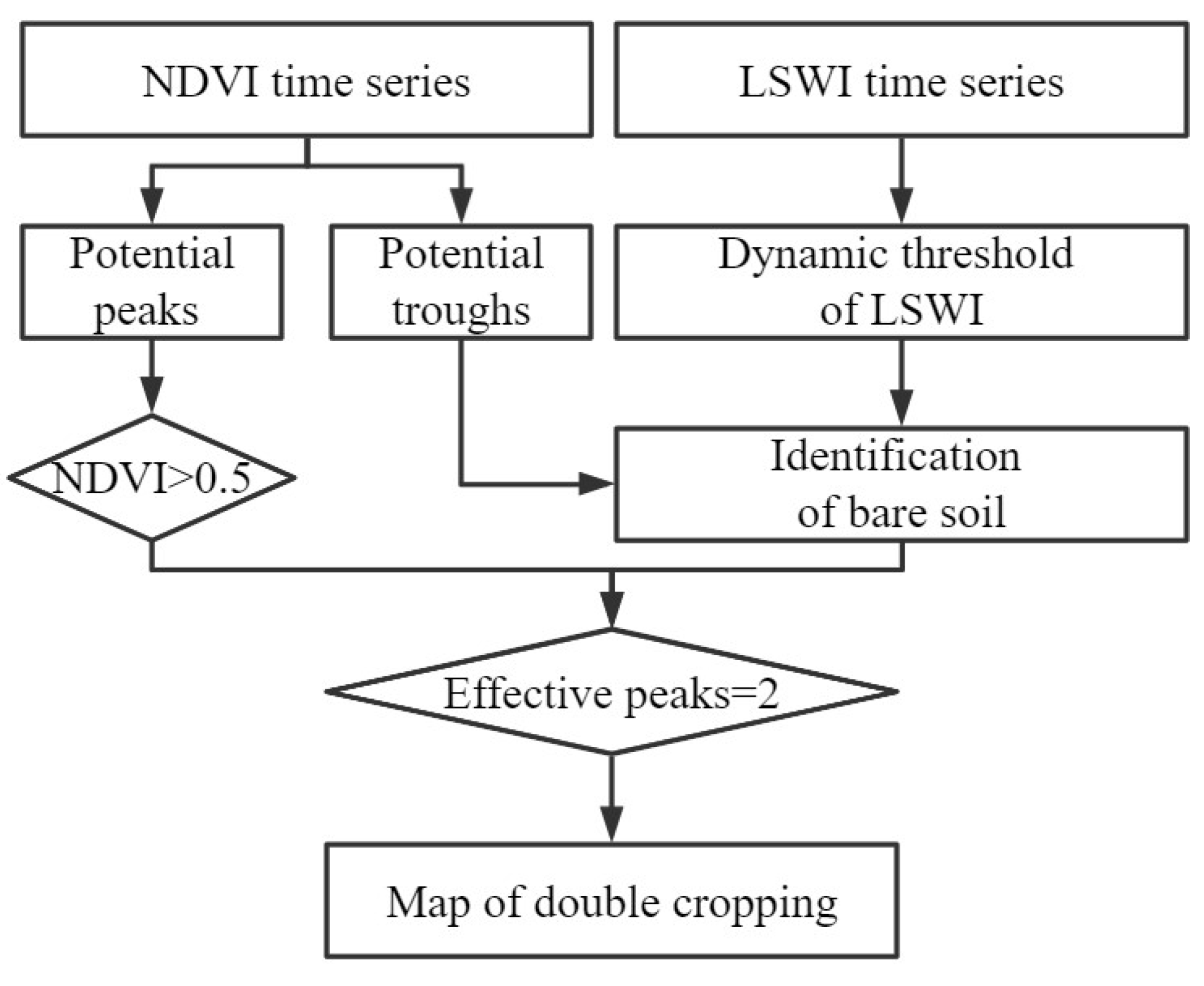
The peak detection method was used to detect the peak (maximum value of adjacent NDVI) and trough (minimum value of adjacent NDVI) in the NDVI time series. Previous studies have shown that the peak growth for crops occurs when NDVI > 0.5, and a fake peak value does not meet this condition [26,36]. Therefore, this condition was used to eliminate fake peaks in the crop growth cycle. According to the difference in soil moisture content from northern to southern China, the LSWI of bare soil varies from 0 to 0.2 [18,37,38]. Therefore, the dynamic threshold method (Equations (3) and (4)) was used to identify the bare soil in the trough period [26]. When bare soil was identified in the two trough periods adjacent to the peak, the peak is marked as an effective peak, that is, it corresponds to a cropping cycle.
where is the potential LSWI threshold and is the final LSWI threshold that is used to identify the bare soil signals. and are the minimum and maximum LSWI values for each period.
Based on the above rules, the number of annual effective peaks was counted for the individual pixels, and the double-cropping maps of 2001, 2005, 2010, 2015, and 2020 were generated, respectively. The steps of the algorithm are shown in Figure 7.
2.3.2. Accuracy Assessment of the Resultant Annual Maps
As the double-cropping maps of different years were obtained from the same algorithm, the classification accuracies of these maps are comparable. Additionally, obtaining samples from earlier years is difficult. Therefore, only the 2020 double-cropping map was assessed. The ground reference datasets obtained in Section 2.2.3 and the double-cropping map (2020) generated by our study were used to construct a confusion matrix to evaluate the potential of the proposed algorithm. The assessment metrics include overall accuracy (OA), user accuracy (UA), producer accuracy (PA), and Kappa coefficient [39].
2.3.3. Extraction of the NLDC
KDE is a nonparametric statistical method for estimating the probability density in geospatial and geographic information analysis [40,41]. KDE can perform a smooth estimation by probability density function according to the location information of sampling points, making the visualization of discontinuous points smoother [42,43]. The KDE was used to extract NLDC, which is defined as follows:
where is the probability density estimator, n is the number of double-cropping points, h(h > 0) is a user-defined smoothing parameter or bandwidth, K is a user-defined non-negative kernel function, is a coordinate vector of estimated points, and is a coordinate vector of sample points.
Bandwidth is an important output parameter in the KDE method, which determines the quality of the KDE [44]. Small bandwidth values will lead to sharp estimates, and the density curve will be too abrupt and scattered, while large bandwidth values will lead to an excessively smooth density curve. Therefore, the appropriate bandwidth value is particularly important for the resultant maps. Three different bandwidths (5 km, 10 km, and 15 km) were compared and analyzed for kernel density values (Figure 8). The 5 km bandwidth curve was too fragmented to reflect the situation of the core fields of double cropping, while the 15 km bandwidth curve was too smooth to ignore the distribution of the double-cropping sparse fields and non-double-cropping fields. Therefore, the optimal bandwidth for NLDC extraction was determined to be 10km in this study.
The NLDC extraction process can be summarized into three steps, which were finalized using ArcGIS. First, the raster cells of double cropping obtained in Section 2.3.1 were converted into point features as input parameters for KDE. Second, the density map of double cropping was obtained according to KDE and optimal bandwidth (10 km). Finally, the percentage-based method was used to determine the kernel density estimation threshold of the 95th percentile [45], and the NLDC was extracted using the contour tool.
2.3.4. Spatial-Temporal Dynamics of the NLDC
The Fishnet method determines the direction and distance of limit movement based on the attributes of the intersection point between the limit and the fishnet [41,46]. To analyze the movement characteristics of NLDC in different directions and periods, a 5 km × 5 km fishnet was generated over the study area, and the intersection points of NLDC and the fishnet in different periods were recorded. When the difference between the latitude coordinates of the current and latter periods was positive (negative), it meant that the NLDC is moving south (north). When the difference between the longitude coordinates of the current and latter periods was positive (negative), it meant that the NLDC was moving west (east). If the difference between the coordinates of the intersection of the two periods was 0, then the NLDC did not move. Equation (6) was used to detect the movement in T1–T5.
where is the former period, is the latter period, is the distance of the NLDC moved, is the coordinate of the intersection point in the former period, and is the coordinate of the intersection point in the latter period.
3. Results
3.1. Accuracy Assessment of Double-Cropping Maps
The obtained 284 (993 pixels) double-cropping sample polygons and 73 (1864 pixels) non-double-cropping sample polygons were used to construct the confusion matrix, as shown in Table 2. The OA, UA, and PA of the 2020 double-cropping map were 95.97%, 96.58%, and 92.21%, respectively, which indicated high classification accuracy. The Kappa coefficient of 0.91 indicated that the classification results were consistent with the ground reference datasets.
3.2. Maps of Double Cropping
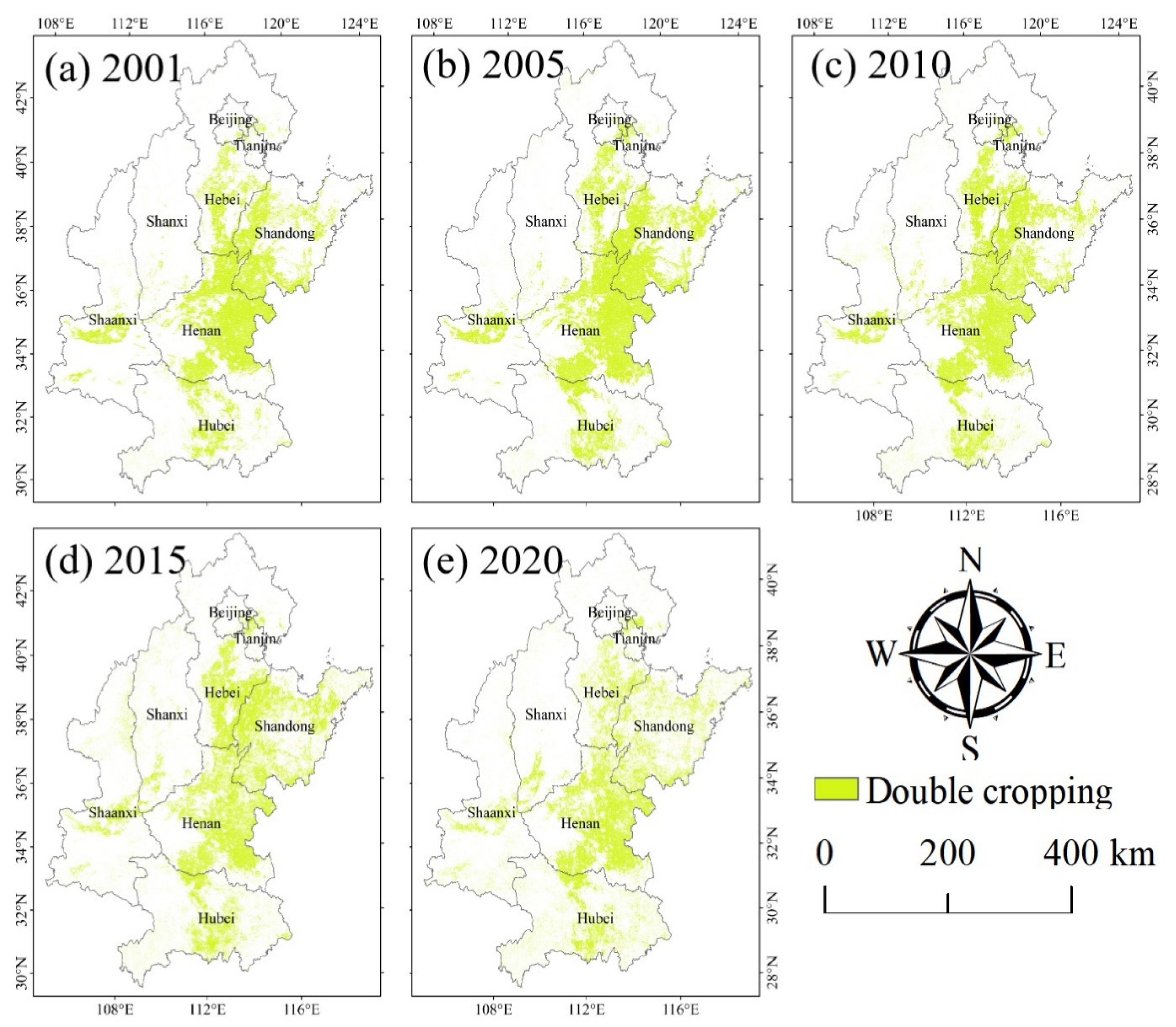
As described in Section 2.3.1, the number of effective peaks of cropland pixels was determined by analyzing MOD09GA NDVI and LSWI time series in the T1–T5 period. Double-cropping maps for 2001, 2005, 2010, 2015, and 2020 were generated using the farmland pixels with a double peak (Figure 9). Generally, the area of double-cropping fields fluctuated up and down in the period T1–T5. In 2001, 2005, 2010, 2015, and 2020, 70.17%, 76.89%, 69.33%, 78.27%, and 66.15%, respectively, of the croplands were double-cropping fields (Table 3). The spatial distribution of double cropping was strongly consistent with topographic characteristics. Hebei Province, Henan Province, and Shandong Province have flat terrain and were where the double-cropping fields were mainly distributed, which accounted for more than half of the double-cropping fields in the study area.
3.3. Spatial-Temporal Dynamics of the NLDC
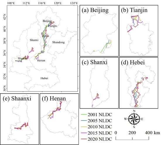
The NLDC is visualized as described in Section 2.3.3 (Figure 10). The NLDC traversed Beijing, Tianjin, Shaanxi, Shanxi, Hebei, and Henan provinces, and generally had a negative trend from the eastern high latitude to the western low latitude. In terms of the moving regions, the NLDC had an obvious trend in Beijing, Tianjin, Shanxi, and Hebei provinces. In terms of the years of the movement, the NLDC movement trend was obvious between 2010–2015 and 2015–2020.
The method described in Section 2.3.4 was used to quantify the north-south and east-west movement of the NLDC (Figure 11 and Figure 12). In the north-south direction, the NLDC fluctuated southward during the periods 2001–2005, 2005–2010, and 2010–2015, and there was a slight northward movement during the period 2015–2020 (Figure 11). During the periods 2001–2005, 2005–2010, and 2010–2015, the NLDC moved south by an average of 1.20 km, 0.30 km, and 6.83 km, respectively. The southward movement mainly occurred in Beijing, Hebei, and Henan provinces, with a maximum shift of 41.15 km, 51.33 km, and 66.60 km, respectively. During the period 2015–2020, the NLDC moved 6.35 km northward on average, mainly in Henan Province, with a maximum of 55.60 km.
In the east-west direction, the NLDC fluctuated eastward during the periods 2001–2005, 2010–2015, and 2015–2020, and there was a slight westward movement during the period 2005–2010 (Figure 12). During the periods 2001–2005, 2010–2015, and 2015–2020, the NLDC moved 5.78 km, 0.44 km, and 18.96 km, respectively, eastward, on average. The eastward movement mainly occurred in Hebei Province, with the farthest movement of 109.52 km. During the period 2005–2010, the NLDC moved westward by 3.67 km on average, mainly in Hebei Province, with a maximum of 52.12 km.
4. Discussion
4.1. Annual Map of Double-Cropping Croplands over Large Spatial Domains
The increasing public availability of satellite data archives and free access to cloud-based geospatial computing platforms such as the Google Earth Engine (GEE) provide unprecedented opportunities to determine cropping intensity over large scales. Several studies have tried to identify the cropping intensity using the peak detection method [26,47,48]. However, most existing efforts have focused on only one specific small region or one specific year, which would limit the application of cropping intensity maps due to the fact that the ability of the method to migrate in spatial-temporal terms has not yet been examined. Additionally, knowledge regarding the multi-year dynamics of the northern limit of cropping intensity is still poor.
Here, we used multi-year MODIS data as well as a phenology-based algorithm to generate double-cropping maps for the major grain producing regions in China. Specifically, each crop growth cycle was identified using the simple principle that bare soil must be present before sowing and after harvesting, which can be determined by the LSWI.
4.2. Analysis of Driving Factors for Shifts of the NLDC
Our analysis indicated that the NLDC showed a general trend of moving south and east during the period 2001–2020 in northern China. However, this does not seem to be consistent with climate change trends. Generally, the limit moves northward during warm and wet periods, and southward during cold and dry periods [49]. Growing season temperatures have increased significantly over the past few decades [50,51], while, more and more arid areas are getting wetter [52,53]. This makes it possible to implement double-cropping systems at higher latitudes, indicating that the climatic resource conditions suitable for double cropping are gradually expanding northwards. The resulting advance of SDT10 and delay of EDT10 were both the main factors that affected the spatial distribution of potential cropping systems [13,14,54], but these do not apply to the NLDC.
The interaction of human activities and climate change provides insights into the movement of the NLDC. Particularly, human activities play a major role in the formation and change of NLDC. For example, the out-migration of agricultural labor [55,56]. As a result of rural-to-urban population migration, the double-cropping system of cropland decreased along with cropland abandonment, especially in low-quality croplands in the hilly rural and mountainous regions [55,57]. It is difficult to implement mechanized operations in mountainous and hilly terrain [58,59]. Additionally, the aging of the agricultural labor force would have an impact on maintaining the present double-cropping system [56].
A series of agricultural stimulation policies since the start of the 21st century have also helped drive the movement of NLDC, including the elimination of the agricultural tax, increased agricultural subsidies, and increased grain price [4,57]. Since 2002, China has carried out agricultural tax reform in Hebei, Shandong, Henan, and Hubei provinces, which to some extent increased farmers’ production enthusiasm [60] and caused the NLDC to move slightly westward after 2005. Due to the lack of groundwater and rainfall in winter, since 2014, Hebei Province has implemented a policy of “one cropping for fallow, one cropping for rainfed”. As a result, a large number of croplands have changed from double cropping to the single cropping of soybeans, peanuts, and cotton [26]. Therefore, The NLDC of Hebei province moved obviously eastward after 2015. Additionally, the Grain for Green Project (GGP) has converted a large amount of cropland to woodland and grassland since 1999, with Shaanxi and Hebei being the main provinces where this policy was implemented [61].
The NLDC movement in Beijing and Tianjin may be attributed to socioeconomic factors [59,62]. In the past 20 years, the cropland abandonment process was spatial-temporally coupled with urbanization, and urbanization has been found to be the main cause of farmland abandonment in suburban fields, especially high-quality cropland [57]. Shaanxi and Shanxi provinces are inland of northwest China, where the climate is dry and ecosystems are fragile. Therefore, water resources and cropland quality are the main factors affecting NLDC movement.
4.3. Uncertainties
Several issues of our analysis must be given attention. First, the errors present in the double-cropping maps would affect the NLDC extraction, including data errors introduced by the MODIS dataset [63,64], the cropland extent dataset, and algorithm errors introduced by differences in vegetation type and climate. Second, we used the kernel density estimation threshold of 95th percentile to extract the NLDC, due to the relatively large area of double-cropping fields that we mainly focused on. There are still very few sporadic fields of double cropping that remain uncovered.
5. Conclusions
The northern limit of double cropping (NLDC) was firstly introduced as a critical indicator of agricultural shifts in China. It is crucial to understand the spatial-temporal shifts of the NLDC in order to develop adaptation strategies and ensure food security in China. Time-series NLDC maps were used to evaluate the spatial-temporal dynamics of double cropping in Northeast China. Here, we used MOD09GA Version 6 data to construct crop growth time series curves that reflected the phenology and growth cycles. We extracted double-cropping fields by determining the number of effective peaks of the time series. The total accuracy of our double-cropping maps was 95.97%, and the Kappa coefficient was 0.91. A novel method was proposed to divide the northern limit of double cropping, which provided a new empirical research method for the study of crop planting limits. Our results showed that the movement of the NLDC trended south and east. The NLDC contributes to the understanding of adaptation and feedback within agricultural production systems, which is essential to ensure sustainable and equitable development of food systems in the future.
Author Contributions
Conceptualization, H.X.; methodology, Y.G. and H.X.; validation, Y.G., H.X., L.P., X.Z., and R.L.; formal analysis, Y.G.; investigation, Y.G., L.P., X.Z., and R.L.; resources, Y.G. and H.X.; data curation, Y.G. and H.X.; writing—original draft preparation, Y.G.; writing—review and editing, Y.G. and H.X.; visualization, Y.G.; funding acquisition, H.X. All authors have read and agreed to the published version of the manuscript.
Funding
This research was funded by the National Natural Science Foundation Project of China (32130066), the Henan Provincial Department of Science and Technology Research Project (212102310019), the Natural Science Foundation of Henan (202300410531), the Youth Science Foundation Program of Henan Natural Science Foundation (202300410077), and the Collaborative Innovation Center on Yellow River Civilization jointly built by Henan Province and the Ministry of Education (2020M19).
Data Availability Statement
MOD09GA Version 6 data are openly available via the Google Earth Engine.
Acknowledgments
We are grateful to the anonymous reviewers whose constructive suggestions have improved the quality of this study. We thank Doughty, Russell B. from the California Institute of Technology for editing the English language to eliminate possible grammatical or spelling errors and to conform to correct scientific English. We express our gratitude to the USGS and GEE platforms for supplying Sentinel data, and to the Dabieshan National Observation and Research Field Station of Forest Ecosystem at Henan for supplying equipment.
Conflicts of Interest
The authors declare no conflict of interest.
References
- Wu, W.; Yu, Q.; You, L.; Chen, K.; Tang, H.; Liu, J. Global cropping intensity gaps: Increasing food production without cropland expansion. Land Use Policy 2018, 76, 515–525. [Google Scholar] [CrossRef]
- Kastner, T.; Rivas, M.J.I.; Koch, W.; Nonhebel, S. Global changes in diets and the consequences for land requirements for food. Proc. Natl. Acad. Sci. USA 2012, 109, 6868–6872. [Google Scholar] [CrossRef] [PubMed] [Green Version]
- D’Amour, C.B.; Reitsma, F.; Baiocchi, G.; Barthel, S.; Güneralp, B.; Erb, K.-H.; Haberl, H.; Creutzig, F.; Seto, K.C. Future urban land expansion and implications for global croplands. Proc. Natl. Acad. Sci. USA 2017, 114, 8939–8944. [Google Scholar] [CrossRef] [PubMed] [Green Version]
- Yan, H.; Liu, F.; Qin, Y.; Doughty, R.; Xiao, X. Tracking the spatio-temporal change of cropping intensity in China during 2000–2015. Environ. Res. Lett. 2019, 14, 035008. [Google Scholar] [CrossRef]
- Zuo, L.; Wang, X.; Zhang, Z.; Zhao, X.; Liu, F.; Yi, L.; Liu, B. Developing grain production policy in terms of multiple cropping systems in China. Land Use Policy 2014, 40, 140–146. [Google Scholar] [CrossRef]
- Mauser, W.; Klepper, G.; Zabel, F.; Delzeit, R.; Hank, T.; Putzenlechner, B.; Calzadilla, A. Global biomass production potentials exceed expected future demand without the need for cropland expansion. Nat. Commun. 2015, 6, 8946. [Google Scholar] [CrossRef] [Green Version]
- Löw, F.; Biradar, C.; Dubovyk, O.; Fliemann, E.; Akramkhanov, A.; Narvaez Vallejo, A.; Waldner, F. Regional-scale monitoring of cropland intensity and productivity with multi-source satellite image time series. GISci. Remote Sens. 2018, 55, 539–567. [Google Scholar] [CrossRef]
- Liu, L.; Xu, X.; Zhuang, D.; Chen, X.; Li, S. Changes in the potential multiple cropping system in response to climate change in China from 1960–2010. PLoS ONE 2013, 8, e80990. [Google Scholar] [CrossRef]
- Ding, M.; Chen, Q.; Xin, L.; Li, L.; Li, X. Spatial and temporal variations of multiple cropping index in China based on SPOT-NDVI during 1999–2013. Acta Geogr. Sin. 2015, 70, 1080–1090. [Google Scholar] [CrossRef]
- Yang, X.; Chen, F.; Lin, X.; Liu, Z.; Zhang, H.; Zhao, J.; Li, K.; Ye, Q.; Li, Y.; Lv, S. Potential benefits of climate change for crop productivity in China. Agric. For. Meteorol. 2015, 208, 76–84. [Google Scholar] [CrossRef]
- Wu, W.-B.; Yu, Q.-Y.; Peter, V.H.; You, L.-Z.; Peng, Y.; Tang, H.-J. How could agricultural land systems contribute to raise food production under global change? J. Integr. Agric. 2014, 13, 1432–1442. [Google Scholar] [CrossRef]
- Zhang, J.; Feng, L.; Yao, F. Improved maize cultivated area estimation over a large scale combining MODIS–EVI time series data and crop phenological information. ISPRS J. Photogramm. Remote Sens. 2014, 94, 102–113. [Google Scholar] [CrossRef]
- Zhang, G.; Dong, J.; Zhou, C.; Xu, X.; Wang, M.; Ouyang, H.; Xiao, X. Increasing cropping intensity in response to climate warming in Tibetan Plateau, China. Field Crops Res. 2013, 142, 36–46. [Google Scholar] [CrossRef]
- Liu, X.; Liu, Y.; Liu, Z.; Chen, Z. Impacts of climatic warming on cropping system borders of China and potential adaptation strategies for regional agriculture development. Sci. Total Environ. 2021, 755, 142415. [Google Scholar] [CrossRef] [PubMed]
- Li, L.; Friedl, M.A.; Xin, Q.; Gray, J.; Pan, Y.; Frolking, S. Mapping crop cycles in China using MODIS-EVI time series. Remote Sens. 2014, 6, 2473–2493. [Google Scholar] [CrossRef] [Green Version]
- Yan, H.; Xiao, X.; Huang, H.; Liu, J.; Chen, J.; Bai, X. Multiple cropping intensity in China derived from agro-meteorological observations and MODIS data. Chin. Geogr. Sci. 2014, 24, 205–219. [Google Scholar] [CrossRef] [Green Version]
- Chen, Y.; Lu, D.; Moran, E.; Batistella, M.; Dutra, L.V.; Sanches, I.D.A.; da Silva, R.F.B.; Huang, J.; Luiz, A.J.B.; de Oliveira, M.A.F. Mapping croplands, cropping patterns, and crop types using MODIS time-series data. Int. J. Appl. Earth Obs. Geoinf. 2018, 69, 133–147. [Google Scholar] [CrossRef]
- Biradar, C.M.; Xiao, X. Quantifying the area and spatial distribution of double-and triple-cropping croplands in India with multi-temporal MODIS imagery in 2005. Int. J. Remote Sens. 2011, 32, 367–386. [Google Scholar] [CrossRef]
- Galford, G.L.; Mustard, J.F.; Melillo, J.; Gendrin, A.; Cerri, C.C.; Cerri, C.E. Wavelet analysis of MODIS time series to detect expansion and intensification of row-crop agriculture in Brazil. Remote Sens. Environ. 2008, 112, 576–587. [Google Scholar] [CrossRef]
- Xiang, M.; Yu, Q.; Wu, W. From multiple cropping index to multiple cropping frequency: Observing cropland use intensity at a finer scale. Ecol. Indic. 2019, 101, 892–903. [Google Scholar] [CrossRef]
- Liu, S.; Ma, X.; Li, Y.; Zhang, P. Farmland cropping system identification in China based on a sliding segmentation algorithm. Resour. Sci. 2014, 36, 1969–1976. [Google Scholar]
- Canisius, F.; Turral, H.; Molden, D. Fourier analysis of historical NOAA time series data to estimate bimodal agriculture. Int. J. Remote Sens. 2007, 28, 5503–5522. [Google Scholar] [CrossRef]
- Panigrahy, S.; Upadhyay, G.; Ray, S.S.; Parihar, J.S. Mapping of cropping system for the Indo-Gangetic plain using multi-date SPOT NDVI-VGT data. J. Indian Soc. Remote Sens. 2010, 38, 627–632. [Google Scholar] [CrossRef]
- Jain, M.; Mondal, P.; DeFries, R.S.; Small, C.; Galford, G.L. Mapping cropping intensity of smallholder farms: A comparison of methods using multiple sensors. Remote Sens. Environ. 2013, 134, 210–223. [Google Scholar] [CrossRef] [Green Version]
- Tan, M.; Robinson, G.M.; Li, X.; Xin, L. Spatial and temporal variability of farm size in China in context of rapid urbanization. Chin. Geogr. Sci. 2013, 23, 607–619. [Google Scholar] [CrossRef] [Green Version]
- Liu, L.; Xiao, X.; Qin, Y.; Wang, J.; Xu, X.; Hu, Y.; Qiao, Z. Mapping cropping intensity in China using time series Landsat and Sentinel-2 images and Google Earth Engine. Remote Sens. Environ. 2020, 239, 111624. [Google Scholar] [CrossRef]
- Liu, C.; Zhang, Q.; Tao, S.; Qi, J.; Ding, M.; Guan, Q.; Wu, B.; Zhang, M.; Nabil, M.; Tian, F. A new framework to map fine resolution cropping intensity across the globe: Algorithm, validation, and implication. Remote Sens. Environ. 2020, 251, 112095. [Google Scholar] [CrossRef]
- Gorelick, N.; Hancher, M.; Dixon, M.; Ilyushchenko, S.; Thau, D.; Moore, R. Google Earth Engine: Planetary-scale geospatial analysis for everyone. Remote Sens. Environ. 2017, 202, 18–27. [Google Scholar] [CrossRef]
- Tucker, C.J. Red and photographic infrared linear combinations for monitoring vegetation. Remote Sens. Environ. 1979, 8, 127–150. [Google Scholar] [CrossRef] [Green Version]
- Xiao, X.; Boles, S.; Liu, J.; Zhuang, D.; Frolking, S.; Li, C.; Salas, W.; Moore III, B. Mapping paddy rice agriculture in southern China using multi-temporal MODIS images. Remote Sens. Environ. 2005, 95, 480–492. [Google Scholar] [CrossRef]
- Griffiths, P.; Nendel, C.; Hostert, P. Intra-annual reflectance composites from Sentinel-2 and Landsat for national-scale crop and land cover mapping. Remote Sens. Environ. 2019, 220, 135–151. [Google Scholar] [CrossRef]
- Kandasamy, S.; Baret, F.; Verger, A.; Neveux, P.; Weiss, M. A comparison of methods for smoothing and gap filling time series of remote sensing observations–application to MODIS LAI products. Biogeosciences 2013, 10, 4055–4071. [Google Scholar] [CrossRef] [Green Version]
- Pan, L.; Xia, H.; Zhao, X.; Guo, Y.; Qin, Y. Mapping Winter Crops Using a Phenology Algorithm, Time-Series Sentinel-2 and Landsat-7/8 Images, and Google Earth Engine. Remote Sens. 2021, 13, 2510. [Google Scholar] [CrossRef]
- Jun, C.; Ban, Y.; Li, S. Open access to Earth land-cover map. Nature 2014, 514, 434. [Google Scholar] [CrossRef] [Green Version]
- Gao, F.; Anderson, M.C.; Zhang, X.; Yang, Z.; Alfieri, J.G.; Kustas, W.P.; Mueller, R.; Johnson, D.M.; Prueger, J.H. Toward mapping crop progress at field scales through fusion of Landsat and MODIS imagery. Remote Sens. Environ. 2017, 188, 9–25. [Google Scholar] [CrossRef] [Green Version]
- Guo, Y.; Xia, H.; Pan, L.; Zhao, X.; Li, R.; Bian, X.; Wang, R.; Yu, C. Development of a New Phenology Algorithm for Fine Mapping of Cropping Intensity in Complex Planting Areas Using Sentinel-2 and Google Earth Engine. ISPRS Int. J. Geo-Inf. 2021, 10, 587. [Google Scholar] [CrossRef]
- Chen, B.; Xiao, X.; Ye, H.; Ma, J.; Doughty, R.; Li, X.; Zhao, B.; Wu, Z.; Sun, R.; Dong, J. Mapping forest and their spatial–temporal changes from 2007 to 2015 in tropical hainan island by integrating ALOS/ALOS-2 L-Band SAR and landsat optical images. IEEE J. Sel. Top. Appl. Earth Obs. Remote Sens. 2018, 11, 852–867. [Google Scholar] [CrossRef]
- Dong, J.; Xiao, X.; Kou, W.; Qin, Y.; Zhang, G.; Li, L.; Jin, C.; Zhou, Y.; Wang, J.; Biradar, C. Tracking the dynamics of paddy rice planting area in 1986–2010 through time series Landsat images and phenology-based algorithms. Remote Sens. Environ. 2015, 160, 99–113. [Google Scholar] [CrossRef]
- Tian, H.; Qin, Y.; Niu, Z.; Wang, L.; Ge, S. Summer Maize Mapping by Compositing Time Series Sentinel-1A Imagery Based on Crop Growth Cycles. J. Indian Soc. Remote Sens. 2021, 49, 2863–2874. [Google Scholar] [CrossRef]
- Peng, J.; Zhao, S.; Liu, Y.; Tian, L. Identifying the urban-rural fringe using wavelet transform and kernel density estimation: A case study in Beijing City, China. Environ. Model. Softw. 2016, 83, 286–302. [Google Scholar] [CrossRef]
- Liang, S.; Wu, W.; Sun, J.; Li, Z.; Sun, X.; Chen, H.; Chen, S.; Fan, L.; You, L.; Yang, P. Climate-mediated dynamics of the northern limit of paddy rice in China. Environ. Res. Lett. 2021, 16, 064008. [Google Scholar] [CrossRef]
- Sims, K.M.; Thakur, G.; Sparks, K.A.; Urban, M.L.; Rose, A.N.; Stewart, R.N. Dynamically-Spaced Geo-Grid Segmentation for Weighted Point Sampling on A Polygon Map Layer; Oak Ridge National Lab(ORNL): Oak Ridge, TN, USA, 2018. [Google Scholar]
- Martínez-Fernández, J.; González-Zamora, A.; Sánchez, N.; Gumuzzio, A.; Herrero-Jiménez, C. Satellite soil moisture for agricultural drought monitoring: Assessment of the SMOS derived Soil Water Deficit Index. Remote Sens. Environ. 2016, 177, 277–286. [Google Scholar] [CrossRef]
- McKenzie, G.; Adams, B. Juxtaposing thematic regions derived from spatial and platial user-generated content. In Proceedings of the 13th international conference on spatial information theory (COSIT 2017), L’Aquila, Italy, 4–8 September 2017. [Google Scholar] [CrossRef]
- Pilø, L.; Finstad, E.; Ramsey, C.B.; Martinsen, J.R.P.; Nesje, A.; Solli, B.; Wangen, V.; Callanan, M.; Barrett, J.H. The chronology of reindeer hunting on Norway’s highest ice patches. R. Soc. Open Sci. 2018, 5, 171738. [Google Scholar] [CrossRef] [PubMed] [Green Version]
- Shi, W.; Liu, Y.; Shi, X. Development of quantitative methods for detecting climate contributions to boundary shifts in farming-pastoral ecotone of northern China. J. Geogr. Sci. 2017, 27, 1059–1071. [Google Scholar] [CrossRef]
- Qiu, B.; Lu, D.; Tang, Z.; Song, D.; Zeng, Y.; Wang, Z.; Chen, C.; Chen, N.; Huang, H.; Xu, W. Mapping cropping intensity trends in China during 1982–2013. Appl. Geogr. 2017, 79, 212–222. [Google Scholar] [CrossRef]
- Pan, L.; Xia, H.; Yang, J.; Niu, W.; Wang, R.; Song, H.; Guo, Y.; Qin, Y. Mapping cropping intensity in Huaihe basin using phenology algorithm, all Sentinel-2 and Landsat images in Google Earth Engine. Int. J. Appl. Earth Obs. Geoinf. 2021, 102, 102376. [Google Scholar] [CrossRef]
- Shi, X.; Shi, W. Review on boundary shift of farming-pastoral ecotone in northern China and its driving forces. Trans. Chin. Soc. Agric. Eng. 2018, 34, 1–11. [Google Scholar]
- Liu, Z.; Liu, Y.; Li, Y. Anthropogenic contributions dominate trends of vegetation cover change over the farming-pastoral ecotone of northern China. Ecol. Indic. 2018, 95, 370–378. [Google Scholar] [CrossRef]
- Zhao, W.; Yang, M.; Chang, R.; Zhan, Q.; Li, Z.L. Surface warming trend analysis based on MODIS/Terra land surface temperature product at Gongga Mountain in the southeastern Tibetan Plateau. J. Geophys. Res. Atmos. 2021, 126, e2020JD034205. [Google Scholar] [CrossRef]
- Donat, M.G.; Lowry, A.L.; Alexander, L.V.; O’Gorman, P.A.; Maher, N. More extreme precipitation in the world’s dry and wet regions. Nat. Clim. Chang. 2016, 6, 508–513. [Google Scholar] [CrossRef]
- Zhao, W.; Wen, F.; Wang, Q.; Sanchez, N.; Piles, M. Seamless downscaling of the ESA CCI soil moisture data at the daily scale with MODIS land products. J. Hydrol. 2021, 603, 126930. [Google Scholar] [CrossRef]
- Shi, W.; Tao, F.; Liu, J.; Xu, X.; Kuang, W.; Dong, J.; Shi, X. Has climate change driven spatio-temporal changes of cropland in northern China since the 1970s? Clim. Chang. 2014, 124, 163–177. [Google Scholar] [CrossRef]
- Yan, J.; Yang, Z.; Li, Z.; Li, X.; Xin, L.; Sun, L. Drivers of cropland abandonment in mountainous areas: A household decision model on farming scale in Southwest China. Land Use Policy 2016, 57, 459–469. [Google Scholar] [CrossRef] [Green Version]
- Li, S.; Li, X. Global understanding of farmland abandonment: A review and prospects. J. Geogr. Sci. 2017, 27, 1123–1150. [Google Scholar] [CrossRef]
- Qiu, B.; Yang, X.; Tang, Z.; Chen, C.; Li, H.; Berry, J. Urban expansion or poor productivity: Explaining regional differences in cropland abandonment in China during the early 21st century. Land Degrad. Dev. 2020, 31, 2540–2551. [Google Scholar] [CrossRef]
- Shi, T.; Li, X.; Xin, L.; Xu, X. Analysis of farmland abandonment at parcel level: A case study in the mountainous area of China. Sustainability 2016, 8, 988. [Google Scholar] [CrossRef] [Green Version]
- Li, S.; Li, X.; Sun, L.; Cao, G.; Fischer, G.; Tramberend, S. An estimation of the extent of cropland abandonment in mountainous regions of China. Land Degrad. Dev. 2018, 29, 1327–1342. [Google Scholar] [CrossRef]
- Huang, J.; Wang, X.; Rozelle, S. The subsidization of farming households in China’s agriculture. Food Policy 2013, 41, 124–132. [Google Scholar] [CrossRef]
- Yuan, W.; Li, X.; Liang, S.; Cui, X.; Dong, W.; Liu, S.; Xia, J.; Chen, Y.; Liu, D.; Zhu, W. Characterization of locations and extents of afforestation from the Grain for Green Project in China. Remote Sens. Lett. 2014, 5, 221–229. [Google Scholar] [CrossRef]
- Wang, Y.; Zhang, J.; Liu, D.; Yang, W.; Zhang, W. Accuracy assessment of GlobeLand30 2010 land cover over China based on geographically and categorically stratified validation sample data. Remote Sens. 2018, 10, 1213. [Google Scholar] [CrossRef] [Green Version]
- Zhao, W.; Li, X.; Wang, W.; Wen, F.; Yin, G. DSRC: An Improved Topographic Correction Method for Optical Remote-Sensing Observations Based on Surface Downwelling Shortwave Radiation. IEEE Trans. Geosci. Remote Sens. 2021. [Google Scholar] [CrossRef]
- Zhao, W.; Duan, S.-B. Reconstruction of daytime land surface temperatures under cloud-covered conditions using integrated MODIS/Terra land products and MSG geostationary satellite data. Remote Sens. Environ. 2020, 247, 111931. [Google Scholar] [CrossRef]
Figure 1.
Land cover (a–c) in 2000, 2010, and 2020; the intersection of cropland in 2000, 2010, and 2020 (d); and topography (e) of the study area. DEM is the abbreviation of digital elevation model.
Figure 1.
Land cover (a–c) in 2000, 2010, and 2020; the intersection of cropland in 2000, 2010, and 2020 (d); and topography (e) of the study area. DEM is the abbreviation of digital elevation model.

Figure 2.
Numbers of good-quality observations at the pixel level during the study period with (a) 2001, (b) 2005, (c) 2010, (d) 2015 and (e) 2020.
Figure 2.
Numbers of good-quality observations at the pixel level during the study period with (a) 2001, (b) 2005, (c) 2010, (d) 2015 and (e) 2020.

Figure 3.
The illustration of the pre-processing of NDVI data. Black circles represent multiple good- quality observations within an 8-day period, red circles represent NDVI maxima within an 8-day period, and solid black lines represent smooth curves.
Figure 3.
The illustration of the pre-processing of NDVI data. Black circles represent multiple good- quality observations within an 8-day period, red circles represent NDVI maxima within an 8-day period, and solid black lines represent smooth curves.

Figure 4.
Distribution of sample points for double and non-double cropping (a). (b–d) show the zoomed-in views of the sample points at (a), corresponding to (b–d) in (a).
Figure 4.
Distribution of sample points for double and non-double cropping (a). (b–d) show the zoomed-in views of the sample points at (a), corresponding to (b–d) in (a).

Figure 5.
Workflow for tracking the spatial-temporal change of the northern limit of double cropping in China. POIs and ROIs represent the points and rasters of interest respectively.
Figure 5.
Workflow for tracking the spatial-temporal change of the northern limit of double cropping in China. POIs and ROIs represent the points and rasters of interest respectively.

Figure 6.
Temporal profile of NDVI for double cropping (a) (114.8096° E, 34.4863° N) and (b) (114.7125° E, 35.3407° N). Cycle 1 and cycle 2 represent a complete growth cycle of the crop.
Figure 6.
Temporal profile of NDVI for double cropping (a) (114.8096° E, 34.4863° N) and (b) (114.7125° E, 35.3407° N). Cycle 1 and cycle 2 represent a complete growth cycle of the crop.

Figure 7.
Workflow for mapping double cropping by MODIS time-series.

Figure 8.
Comparison of the different bandwidth of kernel density for double cropping (a) 5 km, (b) 10 km, (c) 15 km.
Figure 8.
Comparison of the different bandwidth of kernel density for double cropping (a) 5 km, (b) 10 km, (c) 15 km.

Figure 9.
Spatial distribution of double cropping based on MODIS in 2001 (a), 2005 (b), 2010 (c), 2015 (d), and 2020 (e).
Figure 9.
Spatial distribution of double cropping based on MODIS in 2001 (a), 2005 (b), 2010 (c), 2015 (d), and 2020 (e).

Figure 10.
Northern limit of double cropping in 2001, 2005, 2010, 2015, and 2020.

Figure 11.
North-south movement of the double cropping during (a) 2001–2005, (b) 2005–2010, (c) 2010–2015, and (d) 2015–2020.
Figure 11.
North-south movement of the double cropping during (a) 2001–2005, (b) 2005–2010, (c) 2010–2015, and (d) 2015–2020.

Figure 12.
East-west movement of double cropping during (a) 2001–2005, (b) 2005–2010, (c) 2010–2015, and (d) 2015–2020.
Figure 12.
East-west movement of double cropping during (a) 2001–2005, (b) 2005–2010, (c) 2010–2015, and (d) 2015–2020.


Table 1.
The range of T1–T5 and the percentage of corresponding >200 good-quality observations. T1—August 2000 to July 2002, T2—August 2004 to July 2006, T3—August 2009 to July 2011, T4—August 2014 to July 2016, T5—August 2019 to July 2021.
Table 1.
The range of T1–T5 and the percentage of corresponding >200 good-quality observations. T1—August 2000 to July 2002, T2—August 2004 to July 2006, T3—August 2009 to July 2011, T4—August 2014 to July 2016, T5—August 2019 to July 2021.
| Year | Period | Percentage | Year | Period | Percentage | Year | Period | Percentage |
|---|---|---|---|---|---|---|---|---|
| 2000 | T1 | 89.08% | 2009 | T3 | 94.58% | 2018 | ||
| 2001 | 2010 | 2019 | T5 | 95.38% | ||||
| 2002 | 2011 | 2020 | ||||||
| 2003 | 2012 | 2021 | ||||||
| 2004 | T2 | 93% | 2013 | |||||
| 2005 | 2014 | T4 | 94.58% | |||||
| 2006 | 2015 | |||||||
| 2007 | 2016 | |||||||
| 2008 | 2017 |
Table 2.
Results of accuracy assessment for double cropping in 2020.
| Error Matrix (Pixels) | Accuracy (%) | ||||||
|---|---|---|---|---|---|---|---|
| Class | Double | Others | Total | UA | PA | OA | Kappa |
| Double | 959 | 81 | 1040 | 96.58 | 92.21 | 95.97 | 0.91 |
| Others | 34 | 1783 | 1817 | 95.65 | 98.13 | ||
| Total | 993 | 1864 | 2857 | / | / | / | / |
Table 3.
Area statistics of double-cropping map in 2001, 2005, 2010, 2015, and 2020.
| Double-Cropping Fields/km2 | 2001 | 2005 | 2010 | 2015 | 2020 |
|---|---|---|---|---|---|
| Beijing | 777.72 | 895.74 | 637.8750 | 506.82 | 300.99 |
| Tianjin | 764.4 | 1614.34 | 1759.37 | 1746.27 | 1504.95 |
| Hebei | 24,122.97 | 24,552.58 | 29,010.59 | 32,788.19 | 21,388.05 |
| Shaanxi | 12,431.18 | 13,241.76 | 11,633.79 | 14,450.15 | 11,903.73 |
| Shanxi | 2817.24 | 2971.20 | 4078.79 | 7779.98 | 6765.53 |
| Shandong | 44,237.51 | 53,377.09 | 44,768.53 | 51,512.28 | 34,426.19 |
| Henan | 71,661.99 | 75,854.59 | 68,087.11 | 60,217.61 | 63,979.69 |
| Hubei | 20,417.76 | 22,722.65 | 21,717.67 | 26,691.77 | 27,090.54 |
| Total area | 177,154.46 | 206,402.33 | 191,464.90 | 195,108.64 | 166,909.70 |
| Percentage of total farmland area | 70.17% | 76.89% | 69.33% | 78.27% | 66.15% |
Publisher’s Note: MDPI stays neutral with regard to jurisdictional claims in published maps and institutional affiliations. |
© 2022 by the authors. Licensee MDPI, Basel, Switzerland. This article is an open access article distributed under the terms and conditions of the Creative Commons Attribution (CC BY) license (https://creativecommons.org/licenses/by/4.0/).
Share and Cite
MDPI and ACS Style
Guo, Y.; Xia, H.; Pan, L.; Zhao, X.; Li, R. Mapping the Northern Limit of Double Cropping Using a Phenology-Based Algorithm and Google Earth Engine. Remote Sens. 2022, 14, 1004. https://0-doi-org.brum.beds.ac.uk/10.3390/rs14041004
AMA Style
Guo Y, Xia H, Pan L, Zhao X, Li R. Mapping the Northern Limit of Double Cropping Using a Phenology-Based Algorithm and Google Earth Engine. Remote Sensing. 2022; 14(4):1004. https://0-doi-org.brum.beds.ac.uk/10.3390/rs14041004
Chicago/Turabian StyleGuo, Yan, Haoming Xia, Li Pan, Xiaoyang Zhao, and Rumeng Li. 2022. "Mapping the Northern Limit of Double Cropping Using a Phenology-Based Algorithm and Google Earth Engine" Remote Sensing 14, no. 4: 1004. https://0-doi-org.brum.beds.ac.uk/10.3390/rs14041004
Note that from the first issue of 2016, this journal uses article numbers instead of page numbers. See further details here.