Article

A Preliminary Numerical Study to Compare the Physical Method and Machine Learning Methods Applied to GPR Data for Underground Utility Network Characterization

1
Centre for Studies and Expertise on Risks, Environment, Durability, and Urban and Country Planning (Cerema), 23 Av. Amiral Chauvin, 49130 Les Ponts-de-Cé, France
2
Logiroad, 5 Rue de l’Enclose, 44118 La Chevrolière, France
3
Department of Materials and Structures (MAST-LAMES), Université Gustave Eiffel, Nantes Campus, Allée des Ponts et Chaussées, 44340 Bouguenais, France
4
Department of Components and Systems (COSYS-SII), Université Gustave Eiffel, Nantes Campus, Allée des Ponts et Chaussées, 44340 Bouguenais, France
5
Assessment and Imaging Laboratory (GERS-GeoEND), Université Gustave Eiffel, Nantes Campus, Allée des Ponts et Chaussées, 44340 Bouguenais, France
*
Author to whom correspondence should be addressed.
Submission received: 28 January 2022 / Revised: 14 February 2022 / Accepted: 17 February 2022 / Published: 21 February 2022

Abstract

:
In the field of geophysics and civil engineering applications, ground penetrating radar (GPR) technology has become one of the emerging non-destructive testing (NDT) methods thanks to its ability to perform tests without damaging structures. However, NDT applications, such as concrete rebar assessments, utility network surveys or the precise localization of embedded cylindrical pipes still remain challenging. The inversion of geometric parameters, such as depth and radius of embedded cylindrical pipes, as well as the dielectric parameters of its surrounding material, is of great importance for preventive measures and quality control. Furthermore, the precise localization is mandatory for critical underground utility networks, such as gas, power and water lines. In this context, innovative signal processing techniques associated with GPR are capable of performing physical and geometric characterization tasks. This paper evaluates the performance of a supervised machine learning and ray-based methods on GPR data. Support vector machines (SVM) classification, support vector machine regression (SVR) and ray-based methods are all used to correlate information about the radius and depth of embedded pipes with the velocity of stratified media in various numerical configurations. The approach is based on the hyperbola trace emerging in a set of B-scans, given that the shape of the hyperbola varies greatly with pipe depth and radius as well as with velocity of the medium. According to the ray-based method, an inversion of the wave velocity and pipe radius is performed by applying an appropriate nonlinear least mean squares inversion technique. Feature selection within machine learning models is also implemented on the information chosen from observed hyperbola travel times. Simulated data are obtained by means of the finite-difference time-domain (FDTD) method with the 2D numerical tool GprMax. The study is carried out on mono-static, ground-coupled GPR datasets. The preliminary study showed that the proposed machine learning methods outperforms the ray-based method for estimating radius, depth and velocity. SVR, for instance, calculates depth and radius values with mean absolute relative errors of 0.39% and 6.3%, respectively, with regard to the ground truth. A parametric comparison of the aforementioned methodologies is also included in the performance analysis in terms of relative error.

Graphical Abstract

1. Introduction

Ground penetrating radar (GPR) is a non-destructive testing (NDT) method used to both assess the subsurface conditions of a structure and locate buried objects using electromagnetic waves [1]. Thanks to its sensitivity to the material characteristics (such as permittivity, conductivity, etc.), GPR can be used to detect both metallic and non-metallic targets. In addition to the wide range of GPR applications listed in [2], estimating the depth and radius of buried cylindrical pipes has become an important task—for instance, in concrete rebar investigation and underground utility network localization [3]. However, regardless of the information acquired using GPR, each application requires suitable processing techniques in order to interpret GPR data and for decision-making purposes. Within the scope of buried utility pipes, since the 3D localization of underground utility pipes has become mandatory to avoid accidents during excavation, the estimation of depth and radius has been widely studied, as demonstrated in the literature, using the following: the ray-based method [4], full-wave inversion (FWI) [3], Hough transforms [5] and machine learning techniques [6]. Recently, Liu et al. [3] used ray-based and FWI approaches to develop a novel method to estimate radius, depth and relative permittivity of utility pipes. However, the latter approach demands heavy computational resources. Therefore, in order to reduce the complexity, FWI is not considered in this paper.
Within the family of several machine learning algorithms, support vector machines (SVMs) have shown promising results in various applications. Moreover, SVMs have been extended to regression problems via the support vector regression method (SVR). Ihamouten et al. [7] used an SVR-based supervised learning method to determine the correlation between the complex dielectric permittivity and the volumetric water content of hydraulic concretes based on GPR data. In addition, Le Bastard et al. [8] applied SVR to estimate the thin pavement thickness. Furthermore, Todkar et al. [9] used two-class support vector machines (SVM) to detect debonded sections of the pavement structure.
SVM techniques have also displayed promising results for underground utility applications. SVMs serve to detect utilities by automatic hyperbola detection [10]. Notably, Terrasse et al. [11] made use of SVM-based automatic hyperbola detection for utility network detection. In terms of parameter estimation, Kaur et al. [12] focused on the features extracted from rebar hyperbola, whereas Muniappan et al. [6] employed the skeletonization technique to estimate rebar radius and depth in concrete structures. This latter approach however is applied on images and consequently encounters fitting errors on the skeleton compared to the theoretical hyperbola.
The ray-based method was used in [4] to detect buried rebars using inverse problem approach, whereas Li et al. [13] used it to estimate radius of the buried pipe at previously known velocity condition. Dolgiy et al. [14] sought to invert the radius of buried pipes using a ray-based method coupled with least squares fitting techniques. Ristic et al. [15] proposed a nonlinear hyperbola fitting approach to invert the velocity and radius concurrently. Both approaches were developed for mono-static antenna configurations and derived the hyperbola as a function of depth, radius and velocity. Although these methods are promising, the error introduced on the peak localization in the temporal signal leads to large errors in the radius estimation [16].
The depth precision for the mapping of critical underground utility networks such as gas, power and water are regulated by law in countries such as France. For instance, in the case of critical networks, the Class A mandates a maximum inaccuracy of 40 c m . However, it is difficult to estimate the depth precisely since existing methods are not precise to be robust enough to guarantee the desired precision levels. Therefore, the objective of this paper is to provide a preliminary study to compare the physical ray-based and machine learning methods, namely multi-class SVM classification and regression, in order to identify a precise and robust approach to estimate velocity, depth and radius. The proposed objectives are illustrated in Figure 1. The depth ( d i ) from the surface A B to the top of the cylindrical object, the velocity ( v m ) of the surrounding medium of the buried cylindrical objects and the radius ( r i ) of the buried cylindrical objects are the three parameters of interest, as observed in Figure 1.
Due to the lack of suitable experimental data at this stage of the research project, the comparison is drawn on numerical GPR data (B-scan from various configurations) created using the FDTD-based software 2D GprMax [17].
The remainder of this paper is organized as follows: Section 2 presents the two proposed parameter estimation methods, Section 3 reviews the 2D GprMax data models generated to validate the methods, Section 4 presents the results, Section 5 is focused to discussion, and the final section draws a set of conclusions.

2. Estimation Methods

In this paper, three parameters related to embedded pipes were estimated, namely: radius (r), pipe depth (d) and the propagation velocity (v). For this purpose, four approaches have been considered to be broadly categorized into two groups: ray-based and machine learning models. The ray-based method can be implemented in two ways: (1) a concurrent estimation of v, d and r parameters; and (2) a radius (r)-only estimation at a previously known propagation velocity (v) of the medium. This method is performed using an appropriate nonlinear least squares optimization algorithm on the extracted hyperbola with respect to an analytical geometrical ray-based objective function.
To draw a contrast, the machine learning method, namely SVM, has also been implemented as either a multi-class classification model or a regression model, i.e., SVR, in order to estimate the v, d and r parameters.

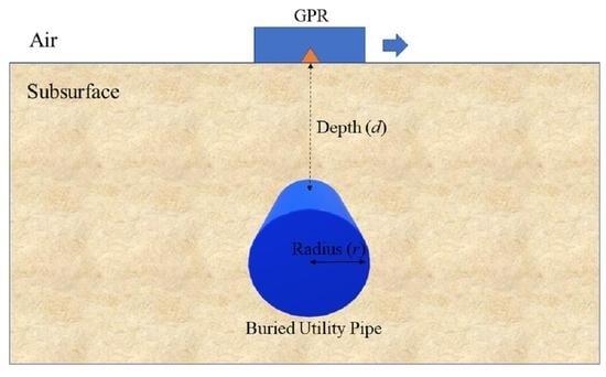
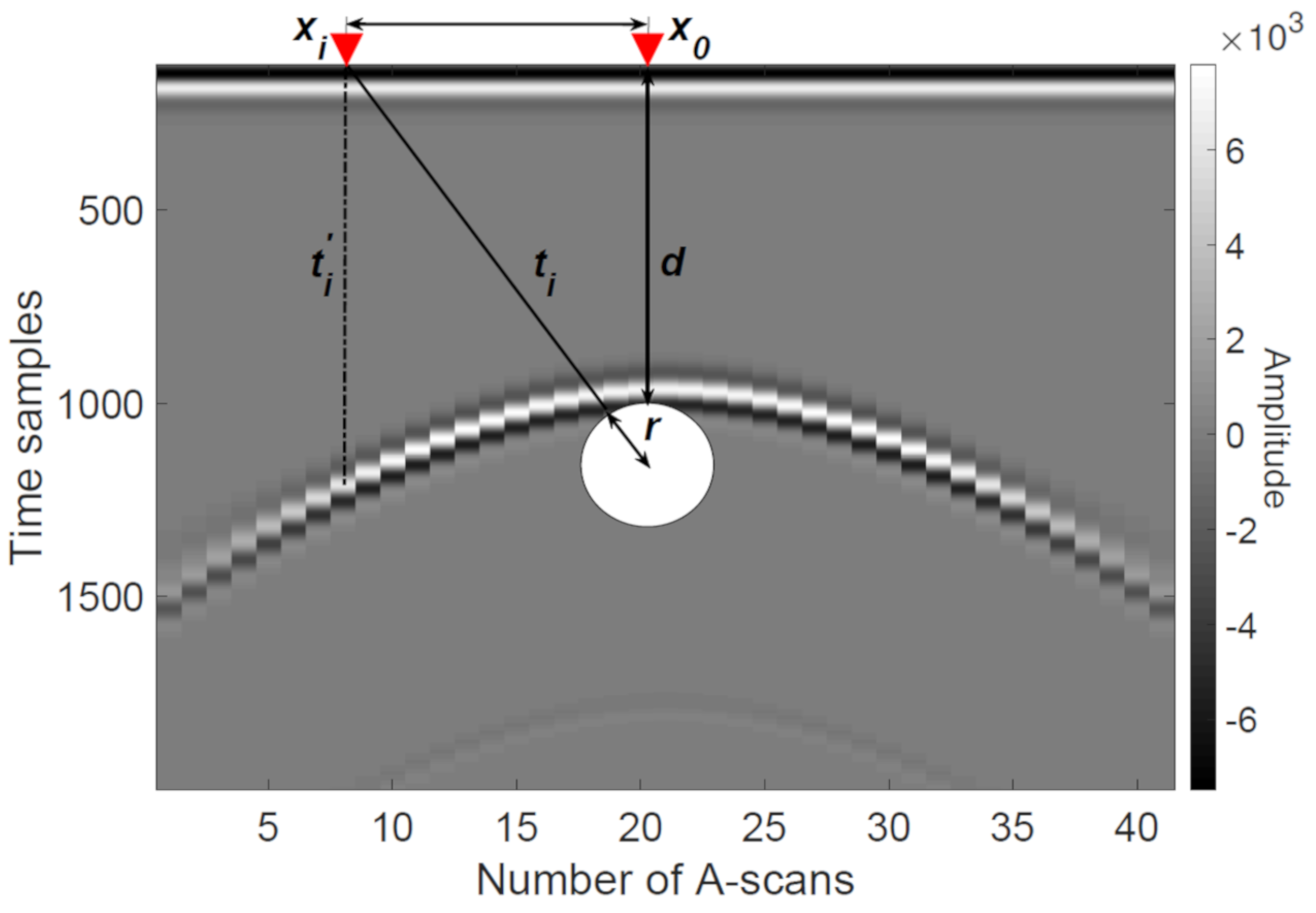
2.1. Ray-Based Method

The hyperbolic signatures in the GPR data are created by reflections occurring on the target surface due to a change in distance between antenna and target.
As shown in Figure 2, in the case of a mono-static antenna configuration—assuming that the reflection takes place on the line between the antenna phase center and the center of the cylinder, when the pipe orientation axis is perpendicular to the horizontal displacement axis of the GPR—the two-way travel time t i of the reflected wave on the cylindrical surface appears at a two-way travel time distance t i on the A-scan of the particular GPR position, such that t i = t i . Hence, the geometrical relationship can be defined in Equation (1) below [4]:
Δ x i 2 = v 2 t i 2 4 + v s . r t i ( d 2 + 2 d r )
where Δ x i 2 = ( x i x 0 ) 2 is derived as a polynomial function of v, r, d and t i , with i denoting the GPR’s horizontal spatial position. From Equation (1), for a given hyperbola, the v, r and d parameters can be inverted since they remain constant, while Δ x i and t i are the variable components. For this step, the unconstrained, Newton quasi-nonlinear optimization algorithm was adopted by virtue of the assumption that the vs. value of the medium remains constant around the hyperbola (a homogeneous and dispersiveness medium without anisotropic properties). The unconstrained solver was chosen given that the inversion results are highly sensitive to both boundary conditions and starting values. In addition, each hyperbola requires fine tuning of the boundary conditions, which proves to be difficult for large datasets with broad configurations in terms of velocity, depth and radius. Hence, the unconstrained, Newton quasi-nonlinear optimization algorithm was adopted to generalize the model and remove its dependence on boundary conditions.
v , d , r = argmin ( ξ , τ , ζ ) i = 1 N Δ x 2 ξ , τ , ζ , t i Δ x i 2 2
where ξ , τ and ζ are the intermediate values of v, d and r, respectively.

2.2. Machine Learning Methods: SVM and SVR

The second family of methods studied in this paper are the SVM and the SVR. These methods are adapted to estimate the v, d and r parameters with three independent trained models. For each parameter inversion, the extracted hyperbola features are considered as inputs, while v, d and r parameters are the predicted values.
While SVM is based on the structural risk minimization principle, SVR is a very specific class of non-parametric regression methods based on SVM. Among two different approaches of SVR, ϵ -SVR is adopted for this study. Multi-class SVM is applied with the perception that the labeled parameters are classified into set of different classes, while SVR is adopted when parameters are considered as continuous value problem.

Formulation

Let T S = { ( z 1 , S 1 ) , , ( z N , S N ) } be composed of N pairs of observation, with z i being the features vector associated with the ith B-scan and S i is the label. In case of radius estimation, we have S i r , for velocity, we have S i v and for depth estimation, we have S i d ; where r, v and d are as defined in the next section. We begin by describing the case of the linear function, f, given by [18]:
f ( z ) = a , z + b   w i t h   z X , b R
where a and b are weight vector and bias, respectively. · , · represents the dot product in X (where X denotes the space of the input patterns).
In case of classification, the optimization problem is expressed as ([9]):
minimize a , b , ξ 1 2 a T a + C i = 1 N ξ i subject   to S i ( a T Φ ( z i ) + b ) 1 ξ i , ξ i 0 , i = 1 , 2 , . . . N .
where Φ is the kernel function that maps vectors into higher dimensional functions, ξ is the slack variable introduced to reduce training errors and C > 0 is the regularization parameter.
The solution f ( x ) uses Lagrange multipliers and is given by [9]:
f ( z ) = s g n i = 1 N S i α i Φ ( z i , z ) + b
where s g n is the sign function, α i are Lagrange multipliers and S i are the class labels.
In case of regression, an additional parameter e is introduced. In addition, in this case ξ and ξ i * are the slack variables included to reduce training errors. Thus, the classification equation can be rewritten as [18]:
minimize a , b , ξ 1 2 a T a + C i = 1 N ( ξ i + ξ i * ) subject   to S i a , z i b e + ξ i , a , z i + b S i e + ξ i * ξ i , ξ i * 0 , i = 1 , 2 , , N
The solution for nonlinear regression given by [18], as follows:
f ( z ) = i = 0 N ( α i α i * ) Φ ( z i , z ) + b
where α i and α i * are Lagrange multipliers. Furthermore, in case of a Gaussian kernel function, Φ can be defined as follows:
Φ ( z , z i ) = e | z z i | 2 2 σ 2
and this is often simplified as
Φ ( z , z i ) = e γ | z z i | 2
where the γ , C and e are optimized in LIBSVM.

2.3. SVM Implementation

Three separate multi-class SVM models ( S V M r , S V M d , S V M v ) and three separate ϵ -SVR models ( S V R r , S V R d , S V R v ) were trained independently with their corresponding labels. Each separate, model-enabled single parameter inversion at a time, solely by relying on the proposed six features. Furthermore, the same set of training and testing data were utilized in all models to avoid any bias in the results due to data set difference.

2.3.1. Feature Selection

The feature selection for the machine learning step is based on the hypothesis that a pipe with a large radius yields flatter hyperbola and the tail of hyperbola is observed to become more parallel in the same medium velocity as observed from experiments (argued by [16]). This pattern correlation relates the hyperbola sector with the three parameters under study namely, v, d and r.
Figure 3, Figure 4 and Figure 5 illustrate how the hyperbola shape varies across different v, d and r. Based on this fact, the features were selected to fully represent the hyperbola shape while minimizing the dimension of the features.
In this context, the B-scan data are initially preprocessed to obtain the six features ( t a , t b , t c , t d , t e , t f ), as shown in Figure 6. These features are described as follows: t a is the two-way travel time from the ground to the vertex of hyperbola, t b is the mean of first 25 of hyperbola data points, t c is the mean of 25 to 75 of hyperbola data points, t d is the mean of 75 to 100 of hyperbola data points, t f is the maximum travel time within the window and t e is the travel time difference (i.e., t f t a ).
The adopted ray-based and machine learning methods presented hereafter are implemented using resulting B-scan feature sets. In this work, travel time, t, was picked, as shown in Figure 7. In the first echo, the antenna radiation source, ground surface and direct coupling wavelets overlap with each other; whereas, in the second echo, a phase inversion of the signal is observed when the pipe is encountered. Due to this, minimum peak from the first echo and the maximum peak from the second echo are selected.

2.3.2. Training, Validation and Testing

Feature extraction is performed on each B-scan signals to obtain the features matrix Z. The data is then divided into two sets—learning and testing—with learn-to-test ratio 80%:20%. The ratio was chosen as an optimized value in terms of model performance while maximizing the size of training data with reasonable amount of test data. The test data is independent from the learning data. Both SVM and SVR are then implemented using the SVM toolbox in MATLAB 2020a. A k-fold cross validation technique is used (with k = 5 ) in the learning stage to validate the model in the learning phase, avoid over-fitting [9] and provide insight on the model’s behavior to unknown data sets.
A loss function, namely average root mean square error (RMSE), is used to determine the optimal values for each method. While SVM adopted fine Gaussian kernel one-to-one multi-class classification, ϵ -SVR adopted the fine Gaussian kernel. In case of SVM, two parameters, namely c and γ , are optimized, whereas an additional ϵ parameter in case of ϵ -SVR were optimized against the RMSE loss function. In this study, described hyperparameters were optimized using the Bayesian optimization algorithm.

3. Database Generation

In order to validate the proposed estimation approaches, simple homogeneous dispersive 2D GprMax models were used [17]. GprMax is an open source simulation software developed in python environment for forward modeling of GPR that uses finite difference time domain (FDTD) to simulate EM wave propagation solving Maxwell’s equations [17].
In our work, the domain size is defined as 1.0   m × 1.0   m . The domain mesh sizes are Δ x = 2.5 × 10 3   m , Δ y = 2.5 × 10 3   m and the time sampling resolution is Δ t = 5.89 × 10 12   s , which satisfies the Courant, Freidrich and Lewy conditions [17]. In terms of the source, a Hertzian dipole is excited with point source with zero-offset, at height of 5 m m , from the surface. The excitation waveform was the Ricker wavelet, centered at f c =   1.5   G Hz .
The model consists of a metallic cylindrical pipe embedded within a single layer, as described in Figure 2. The permittivity of the layer ( ε r ) is varied between 6 and 16 with steps of 0.33. Cylindrical pipe’s positioning depth (d) varies between 30 c m to 70 c m with incremental steps of 10 c m . The radius of the pipe on the other hand are 1 c m , 2 c m , 3 c m , 5 c m , 7 c m and 10 c m with 3 different conductivity ( σ ) levels at 1 × 10 5   S / m , 1 × 10 3   S / m and 1 × 10 1   S / m . The spatial resolution between adjacent A-scans is 2 c m . Thus, a total of 2610 unique B-scans were created with each B-scan made up of 41 A-scans. Furthermore, the ground truth values of v, d and r for both the training and test sets were obtained from the above-mentioned simulation settings, whereas the ground truth is required either for supervised learning with train data and then to calculate the model’s performance on test data.

4. Results

Table 1 compares the performance results of the mean relative error (mean err) and the maximum relative error in terms of 95th percentile ( P 95 ) were computed using Equation (8):
e r r =   ( M e s t M a c t ) M a c t   ×   100
where M e s t is the estimated value and M a c t is the actual value.
The relative error (err) of the predicted value with reference to its actual value of every tested data (in this case hyperbolas or its features) was estimated. Then, the relative errors (err) are populated for the whole test results in order to obtain the mean relative error (mean err). Like wise, the mean relative error of each parameter estimation (for radius (r), depth (d) and velocity (v)) was calculated separately for every proposed model (ray-based, S V M m and S V R m ), that are presented in Table 1.
Globally, as seen in Table 1, both SVM and SVR show promising results for estimation of v, d and r. SVM shows the highest performance with false alarm of 10/500 for radius estimation, and SVR shows 6.3% mean relative error (err) for continuous value problems in the radius estimation. Among ray-based method, performance of radius estimation is slightly increased when the velocity is pre-known, but not significantly. The obtained mean err of depth (d) and velocity (v) estimation is comparatively very low in the SVR and SVM approach, whereas the err is less than 1%.

5. Discussion

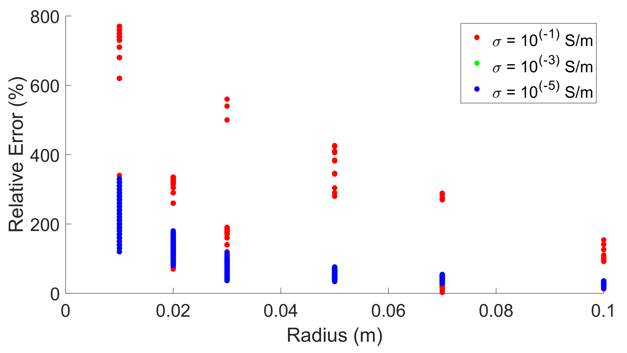
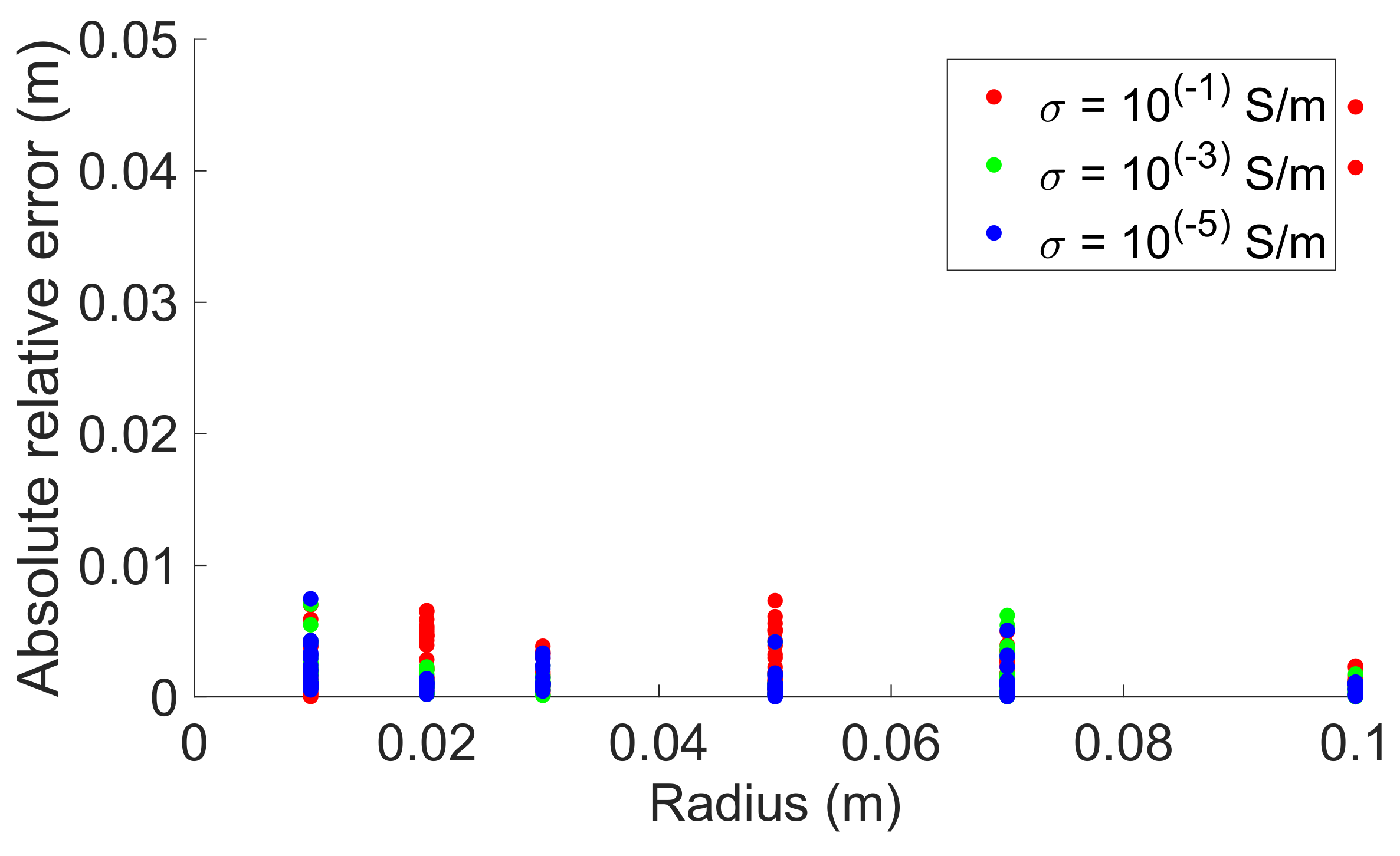
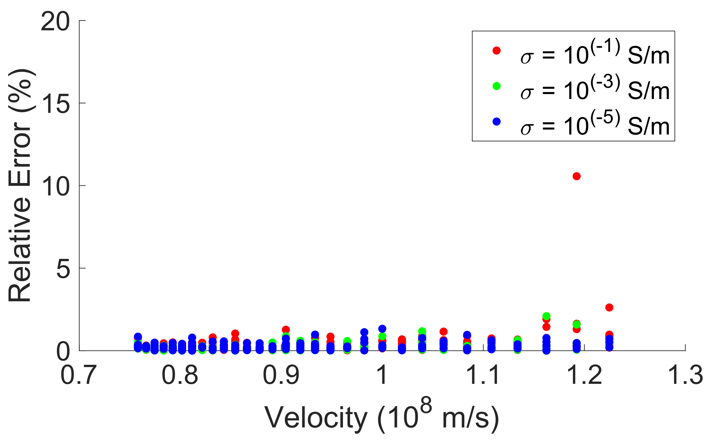
5.1. Ray-Based Method
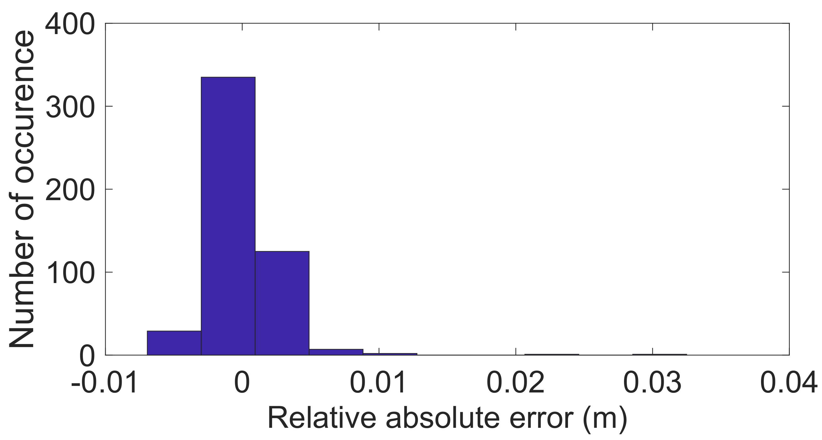
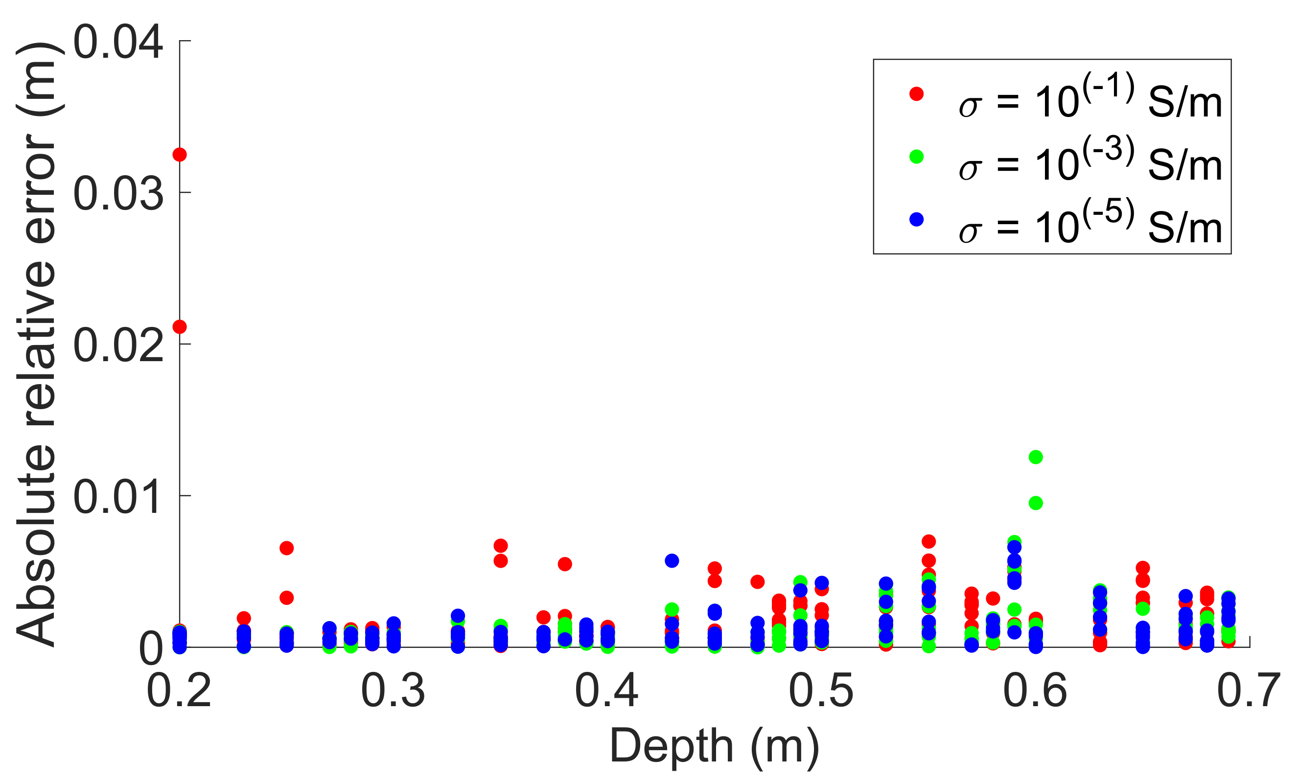
The proposed ray-based parameter estimation method was applied in two different approaches. First, all parameters such as v, d and r were estimated concurrently. Then r was estimated for pre-known values of v and d. Both approaches adhere to the objective function described in Equation (1), followed by the best fit error minimization function mentioned in Equation (2). Hyperbola obtained from numerical B-scans were fitted with analytical objective function to invert the best value of the coefficients, such as v, d and r.
From concurrent ray-based estimation method, means err are 260%, 25.1% and 11.3%, for r, d and v, respectively. Thus, the concurrent parameter estimation’s performance is very poor among all tested methods according to the results in Table 1. However, fixed velocity ray-based method shows relatively better performance for the radius estimation with 120% of mean err. Nevertheless, the mean err is still higher compare to machine learning based methods. The possible contribution of higher uncertainty in ray-based method arises from the bias in the travel time picking and lack of regularization techniques. Furthermore, error increases with medium’s conductivity ( σ ) due to the fact that the pulse’s high frequency components are attenuated by the medium and it cause a shift in the signal peak further resulting in more travel time picking errors.
Additionally, it was observed that the boundary conditions and starting values of the optimization process greatly influence the estimated results. When optimization techniques are applied on broad range of r, d and v configurations with single boundary conditions, the optimization converges at the local minima instead of global minima. Thus, fine tuning of boundary conditions for each hyperbola is required; which is not feasible for broad configurations at this stage. Therefore, considering all above drawbacks, the objective function for the ray-based method must be revised along with more innovative unconstrained optimization techniques to further improve the performance of the ray-based method. Furthermore, the objective function may vary based on the frequency configurations, antenna type and antenna offset of the GPR. Due to the time complexity of further parametric study in this direction, the scope of this study is limited to the proposed objective function.

5.2. SVM

In case of SVM classification, multi class one-to-one SVM classification is adopted as another approach for the proposed estimation problem in this study. In certain applications, such as concrete rebars and certain underground utilities, the depth (d) and radius (r) are being standardized and motivated to implement the multi-class SVM classifier in order to predict the closest possible class. In this context, each design parameter value of v, d and r of the training data set was trained as a classification label so that the model could predict the closest class for an input data. In this context, three separate SVM models were trained for v, d and r. In this respect, the SVM model results shows 1%, 0% and 2% false alarm rates for v, d and r inversions, respectively.
In the radius estimation, as demonstrated in Figure 8, the boxes highlighted in blue indicate correct class predictions while pink boxes correspond to false alarms. SVM’s false alarms are higher at 1 c m and the false alarm rate decreases with the increasing radius size. Noticeably the false alarms are only one class away from the actual value. For example, when the true radius value is 1 c m , the model predicts 96 cases correctly while in 5 cases it falsely classifies as 2 c m . In overall, only 10/500 predictions were found to be false alarms particularly, which come from 1 c m , 2 c m and 3 c m classes with the medium’s relative permittivity range of 6–7 (overall permittivity range of studied data: 6–16). Although the performance of SVM models are better than other approaches, due to the lack of radius standardization between pipe fabricators, it limits the applicability of SVM.

5.3. SVR

The SVR models are trained based on proposed features as a continuous value problem. Three separate SVR models were trained for, respectively, r, d and v, with the same data sets. According to Table 1, its observed that the mean err obtained from SVR models are very low compared with ray-based methods, whereas the estimated means err corresponding to the SVR models are 6.3%, 0.39% and 1% for r, d and v, respectively. According to Figure 9 and Figure 10, the err significantly drops from 120% to 6.3% in case of SVR compared with the ray-based approach. The errors are significantly lowered at larger radius (r) classes and relatively higher at high conductivity ( σ ).
Overall mean err of the radius (r) estimation is 6.3% as seen from Table 1, and based on Figure 11 and Figure 12, radius err shows an increasing trend with depth (d) and the velocity (v), and it is relatively higher when medium’s conductivity ( σ ) level is at 1 × 10 1   S / m .
Referring to the histogram in Figure 13, based on Equation (9), it shows that the linear relative error ( l . r . e ) of the radius estimation varies within the range of −1 to 1 c m ; and from Figure 14, which is based on Equation (10), maximum linear relative absolute error ( a . l . r . e ) is nearly 1 cm, its comparatively low at 10 c m radius class and higher at high-conductivity ( σ ) medium, which is plotted in red.
l . r . e = ( M e s t M a c t )
a . l . r . e = | ( M e s t M a c t ) |
In terms of depth (d) estimation errors in SVR, overall mean err was as low as 0.39% as per Table 1. Furthermore, as shown in Figure 15, the err of the depth (d) estimation remained consistent across the depth classes. Nevertheless, according to Figure 16, the depth (d) estimation error is slightly increasing with the velocity (v). Meanwhile, both figures indicate that depth estimation error is less sensitive to a medium’s conductivity ( σ ) variation in contrast to radius (r) estimation.
Likewise, according to the Figure 17, l.r.e varies approximately between 5   m m and 5 m m , and its increased with higher depth classes as in Figure 18.
Figure 19 and Figure 20 present the velocity estimation’s err variation within different depth (d) and velocity (v) classes, respectively. Overall mean err of velocity estimation remains below 0.5%; however, few outliers were noticed in the lower depth classes from 0.2 m to 0.25 m , but error level is consistent across other depth classes. On the other hand, err is increases slightly with the velocity; however, it does not show any significant variation with medium’s conductivity, except, once again, a few outliers observed in the higher velocity classes.
The impact of the buried medium’s conductivity in the SVR’s model performance was analyzed in terms of mean err at three predefined conductivity levels, such as ( σ ) 1 × 10⁻⁵ S m−1, 1 × 10⁻³ S m−1 and 1 × 10⁻¹ S m−1, which is presented in Table 2. Overall mean err and the 95th percentile of err increases with the conductivity in r, d and v estimations. For example, though the mean err is 6.3% in radius estimation, the error has increased from 5.3% to 7.7% when ( σ ) is increased from 1 × 10⁻⁵ S m−1 to 1 × 10⁻¹ S m−1. However, the error difference is very small between ( σ ) levels 1 × 10⁻⁵ S m−1 and 1 × 10⁻³ S m−1. The trend is similar for both depth d and velocity v as well. However, The depth d and velocity v estimation mean err are well remained below 1%. Radius estimation mean err are larger at higher conductivity medium due to the fact that the pulse’s frequency components are attenuated by the medium and it cause changes in the pulse shape and shifts the signal peak and causes travel time picking error. Since the radius is highly sensitive to the travel time error, it leads to large error in the radius estimation.

6. Conclusions

In this article, we presented a comparative study to analyze the performance of the ray-based method, SVM and SVR to estimate velocity, depth and radius of buried cylindrical pipes. It shows that, in this particular study, with the proposed feature set, the SVM and SVR performances were much better than the ray-based method. A detailed analysis with respect to radius, depth and velocity estimation were presented. The overall results suggests that the depth and velocity estimation accuracy is more robust than the radius inversion in the proposed model. Furthermore, between SVR and SVM, due to the lack of radius standardization between pipe fabricators, it is difficult to obtain a conclusive model for parameter inversion and thereby it constitutes a limit for the applicability of multi-class SVM. The ray-based method suffered from many different factors, including being trapped in the local minima during the optimization. However, its still be a choice for an approximated estimation if objective function and optimization techniques are further modified, accounting all factors discussed in this article, but it requires further study in this direction.
The radius estimation is less accurate compare to other parameters due to fact that radius is highly sensitive to the travel time error, and the support vector region size ( ξ i * ) of SVR is comparable to the RMSE difference between adjacent radius classes, leading to additional error. Even though the machine learning models produce promising results, the availability of large training data set with known design values are still being the challenge for the applicability. Hence, it must be overcome by creating a large experimental data set which is unique to a certain GPR equipment.
In perspective, first the authors propose to perform the analysis on PVC pipes and further on more complex, noisy and realistic data followed by validation of experimental data to evaluate whether uncertainties remain at acceptable level for different applications on specific standards. Authors also propose to modify the ray based objective function with more robust unconstrained optimisation technique. Moreover, authors propose to study the impact of cross validation ratio and database size. Furthermore, artificial neural network approach for the parameter estimation also in the scope of extended study in-order to evaluate if the radius estimation can be further improved compared to SVR.

Author Contributions

This research and development work was carried out in various stages: Conceptualization, methodology, data curation, implementation and validation, writing, editing and review. Conceptualization, methodology, R.M.J.; data curation, R.M.J., D.G. and A.A.; implementation, R.M.J., A.I. and D.G.; validation, R.M.J., A.I., Y.G. and X.D.; writing—original draft preparation, R.M.J.; writing—review and editing, A.I., Shreedhar Savant Todkar and X.D. All authors have read and agreed to the published version of the manuscript.

Funding

This research received no external funding.

Institutional Review Board Statement

Not applicable.

Informed Consent Statement

Not applicable.

Data Availability Statement

Research data are not shared.

Conflicts of Interest

The authors declare no conflict of interest.

References

  1. Lai, W.W.; Dérobert, X.; Annan, P. A review of Ground Penetrating Radar application in civil engineering: A 30-year journey from Locating and Testing to Imaging and Diagnosis. NDT & E Int. 2018, 96, 58–78. [Google Scholar] [CrossRef]
  2. Pajewski, L.; Benedetto, A.; Derobert, X.; Giannopoulos, A.; Loizos, A.; Manacorda, G.; Marciniak, M.; Plati, C.; Schettini, G.; Trinks, I. Applications of Ground Penetrating Radar in civil engineering—COST action TU1208. In Proceedings of the 2013 7th International Workshop on Advanced Ground Penetrating Radar, Nantes, France, 2–5 July 2013; IEEE: Piscataway, NJ, USA, 2013; pp. 1–6. [Google Scholar]
  3. Liu, T.; Klotzsche, A.; Pondkule, M.; Vereecken, H.; Su, Y.; van der Kruk, J. Radius estimation of subsurface cylindrical objects from ground-penetrating-radar data using full-waveform inversion. Geophysics 2018, 83, H43–H54. [Google Scholar] [CrossRef]
  4. Mechbal, Z.; Khamlichi, A. Sensitivity of the inverse problem solution related to detection of rebars buried in concrete by using GPR scanning. In MATEC Web of Conferences; EDP Sciences: Les Ulis, France, 2018; Volume 191, p. 00010. [Google Scholar] [CrossRef]
  5. Windsor, C.; Capineri, L.; Falorni, P. The Estimation of Buried Pipe Diameters by Generalized Hough Transform of Radar Data. In Proceedings of the Proceedings Progress in Electromagnetics Research Symposium (PIERS), Hangzhou, China, 22–26 August 2005; Volume 1, pp. 345–349. [Google Scholar]
  6. Muniappan, N.; Rao, E.P.; Hebsur, A.V.; Venkatachalam, G. Radius estimation of buried cylindrical objects using GPR—A case study. In Proceedings of the 2012 14th International Conference on Ground Penetrating Radar (GPR), Shanghai, China, 4–8 June 2012; pp. 789–794. [Google Scholar] [CrossRef]
  7. Ihamouten, A.; Le Bastard, C.; Xavier, D.; Bosc, F.; Villain, G. Using machine learning algorithms to link volumetric water content to complex dielectric permittivity in a wide (33–2000 MHz) frequency band for hydraulic concretes. Near Surf. Geophys. 2016, 14, 527–536. [Google Scholar] [CrossRef]
  8. Le Bastard, C.; Baltazart, V.; Dérobert, X.; Wang, Y. Support Vector Regression method applied to thin pavement thickness estimation by GPR. In Proceedings of the 2012 14th International Conference on Ground Penetrating Radar (GPR), Shanghai, China, 4–8 June 2012; pp. 349–353. [Google Scholar] [CrossRef]
  9. Todkar, S.S.; Le Bastard, C.; Baltazart, V.; Ihamouten, A.; Dérobert, X. Performance assessment of SVM-based classification techniques for the detection of artificial debondings within pavement structures from stepped-frequency A-scan radar data. NDT & E Int. 2019, 107, 102128. [Google Scholar] [CrossRef]
  10. Terrasse, G.; Nicolas, J.; Trouvé, E.; Drouet, É. Application of the Curvelet Transform for Clutter and Noise Removal in GPR Data. IEEE J. Sel. Top. Appl. Earth Obs. Remote Sens. 2017, 10, 4280–4294. [Google Scholar] [CrossRef]
  11. Terrasse, G.; Nicolas, J.; Trouvé, E.; Drouet, E. Sparse decomposition of the GPR useful signal from hyperbola dictionary. In Proceedings of the 2016 24th European Signal Processing Conference (EUSIPCO), Budapest, Hungary, 29 August–2 September 2016; pp. 2400–2404. [Google Scholar] [CrossRef] [Green Version]
  12. Kaur, P.; Dana, K.J.; Romero, F.A.; Gucunski, N. Automated GPR Rebar Analysis for Robotic Bridge Deck Evaluation. IEEE Trans. Cybern. 2016, 46, 2265–2276. [Google Scholar] [CrossRef] [PubMed]
  13. Li, T.; Zheng, Z. Fast Extraction of Hyperbolic Signatures in GPR. In Proceedings of the 2007 International Conference on Microwave and Millimeter Wave Technology, Guilin, China, 19–21 April 2007; pp. 1–3. [Google Scholar] [CrossRef]
  14. Dolgiy, A.; Dolgiy, A.; Zolotarev, V. GPR Estimation for Diameter of Buried Pipes. In Near Surface 2005, Proceedings of the 11th European Meeting of Environmental and Engineering Geophysics, Palermo, Italy, 4–7 September 2005; European Association of Geoscientists & Engineers: Houten, The Netherlands, 2005; Volume cp-13-00175. [Google Scholar] [CrossRef]
  15. Ristic, A.V.; Petrovacki, D.; Govedarica, M. A new method to simultaneously estimate the radius of a cylindrical object and the wave propagation velocity from GPR data. Comput. Geosci. 2009, 35, 1620–1630. [Google Scholar] [CrossRef]
  16. Borgioli, G.; Capineri, L.; Falorni, P.; Matucci, S.; Windsor, C.G. The Detection of Buried Pipes from Time-of-Flight Radar Data. IEEE Trans. Geosci. Remote Sens. 2008, 46, 2254–2266. [Google Scholar] [CrossRef]
  17. Warren, C.; Giannopoulos, A.; Giannakis, I. gprMax: Open source software to simulate electromagnetic wave propagation for Ground Penetrating Radar. Comput. Phys. Commun. 2016, 209, 163–170. [Google Scholar] [CrossRef] [Green Version]
  18. Smola, A.J.; Schölkopf, B. A tutorial on support vector regression. Stat. Comput. 2004, 14, 199–222. [Google Scholar] [CrossRef] [Green Version]
Figure 1. Buried cylinders in the subsurface and intended estimated parameter.
Remotesensing 14 01047 g001
Figure 2. Geometrical, Ray−based relationship of a buried cylinder.
Remotesensing 14 01047 g002
Figure 3. Examples of hyperbola shape variation across different velocity at same depth and radius.
Remotesensing 14 01047 g003
Figure 4. Examples of hyperbola shape variation across different depth at same velocity and radius.
Remotesensing 14 01047 g004
Figure 5. Examples of hyperbola shape variation across different radii at same velocity and depth.
Remotesensing 14 01047 g005
Figure 6. Representation of travel-time-based feature selection from the hyperbola on a B-scan; ε r = 6 , r = 1   c m , d = 30   c m .
Remotesensing 14 01047 g006
Figure 7. Travel time estimation from A−scan for hyperbola formation.
Remotesensing 14 01047 g007
Figure 8. Confusion matrix of predicted results for radius estimation based on multi-class SVM classification model. Radius classes: 1 cm, 2 cm, 3 cm, 5 cm, 7 cm and 10 c m , respectively. Blue boxes indicates number of correct predictions and pink boxes represents number of false alarms.
Remotesensing 14 01047 g008
Figure 9. Absolute relative error (err) in ray−based estimation of radius at fixed velocity scenario.
Remotesensing 14 01047 g009
Figure 10. Absolute relative error (err) in SVR−based estimation of radius.
Remotesensing 14 01047 g010
Figure 11. Absolute relative error (err) variation in SVR−based radius estimation across different depths.
Remotesensing 14 01047 g011
Figure 12. Absolute relative error (err) variation in SVR−based radius estimation across different velocities of mediums.
Remotesensing 14 01047 g012
Figure 13. SVR−linear relative error (l.r.e) of radius estimation.
Remotesensing 14 01047 g013
Figure 14. SVR−linear absolute relative error (a.l.r.e) of radius estimation.
Remotesensing 14 01047 g014
Figure 15. Absolute relative error (err) variation in SVR−based depth estimation across different depths.
Remotesensing 14 01047 g015
Figure 16. Absolute relative error (err) variation in SVR−based depth estimation across different velocities of mediums.
Remotesensing 14 01047 g016
Figure 17. SVR−linear relative error (l.r.e) of depth estimation.
Remotesensing 14 01047 g017
Figure 18. SVR−linear absolute relative error (a.l.r.e) of depth estimation.
Remotesensing 14 01047 g018
Figure 19. Absolute relative error (err) across depth classes.
Remotesensing 14 01047 g019
Figure 20. SVR−velocity error (err) across velocity classes.
Remotesensing 14 01047 g020
Table 1. Mean relative error and maximum relative error in terms of 95th percentiles ( P 95 ) with respect to radius (r), depth (d) and velocity (v) estimation. The last row represents the number of false alarms in SVM.
Method err ( r ) % err ( d ) % err ( v ) %
Mean P 95 Mean P 95 Mean P 95
Ray-based
concurrent
260%464%25.1%65%11.3%22%
Ray-based
fixed
velocity
120%353%----
Regression
(SVR)
6.3%26.5%0.39%1%0.22%0.5%
Classification
(SVM)
2% (10/500)0% (0/500)1% (5/500)
Table 2. Mean absolute relative error and 95th percentiles ( P 95 ) with respect to radius (r), depth (d) and velocity (v) estimation in SVR approach.
Conductivity ( σ ) err ( r ) % err ( d ) % err ( v ) %
Mean P 95 Mean P 95 Mean P 95
1 × 10⁻⁵ S m−15.3%26.04%0.25%0.74%0.12%0.39%
1 × 10⁻³ S m−1 5.9%25.5%0.26%0.75%0.14%0.42%
1 × 10⁻¹ S m−17.7%28.4%0.52%1.1%0.32%0.79%
Publisher’s Note: MDPI stays neutral with regard to jurisdictional claims in published maps and institutional affiliations.

