Article

Digital Terrain Modelling by Remotely Piloted Aircraft: Optimization and Geometric Uncertainties in Precision Coffee Growing Projects

by
Lucas Santos Santana
1,
Gabriel Araújo e Silva Ferraz
1,
Diego Bedin Marin
1,
Rafael de Oliveira Faria
1,
Mozarte Santos Santana
2,
Giuseppe Rossi
3 and
Enrico Palchetti
4,*
1
Agricultural Engineering Department, Federal University of Lavras, P.O. Box 3037, Lavras 37200-900, MG, Brazil
2
Institute of Natural Sciences, Federal University of Lavras, P.O. Box 3037, Lavras 37200-900, MG, Brazil
3
Department of Agriculture, Food, Environment and Forestry (DAGRI), University of Florence, Via San Bonaventura 13, 50145 Florence, Italy
4
Department of Agricultural, Food, Environment and Forestry (DAGRI), University of Florence, Piazzale Delle Cascine 15, 50144 Florence, Italy
*
Author to whom correspondence should be addressed.
Submission received: 13 January 2022 / Revised: 31 January 2022 / Accepted: 7 February 2022 / Published: 14 February 2022
(This article belongs to the Special Issue New Trends in High Resolution Imagery Processing)

Abstract

:
The implantation of coffee crop plantations requires cartographic data for dimensioning areas and planning the planting line. Digital terrain models (DTMs) obtained from remotely piloted aircraft (RPA) can contribute to efficient data collection for topography making this technique applicable to precision coffee projects. Aiming to achieve efficiency in the collection, processing and photogrammetric products quality, flight configurations and image processing were evaluated. Two hundred sixty-five points obtained by Global Navigation Satellite System (GNSS) receivers characterized the topographic surface. Then eighteen flight missions were carried out by RPA in the configurations of altitude above ground level (AGL) and frontal and lateral image overlay. In addition, different point cloud formats evaluated the image processing (time) efficiency in DTM. Flights performed at 120 m AGL and 80 × 80% overlap showed higher assertiveness and efficiency in generation DTMs. The 90 m AGL flight showed great terrain detail, causing significant surface differences concerning the topography obtained by GNSS. An increase in image overlap requires longer processing times, not contributing linearly to the geometric quality of orthomosaic. Slope ranges up to 20% are considered reliable for precision coffee growing projects; above 20% overestimates the slope values of the land. Changes in flight settings and image processing are satisfactory for precision coffee projects. Image overlap reduction was significant in reducing the processing time without influencing the quality of the DTMs. In addition, image processing performed in shallow point clouds did not interfere with the DTMs quality.

1. Introduction

Coffee growing represents an important source of income for many countries [1]. Brazil leads global coffee production, with its production accounting for 70% of the global supply [2]. Technological advances that relate to growing coffee have contributed to obtaining accurate and reliable measurements of production in the field [3]. Designing and applying techniques that make agricultural production more effective are essential [4]. Thus, smart agriculture practice has become crucial for maximizing yields and preserving natural resources [5].
In coffee regions, planning prior to planting has become indispensable. This crop is mostly grown in mountainous regions, which contributes to increases in errors during the planting stage [6]. Abrupt variations in terrain slope cause a reduction in operational performance and even limitations in machinery use [7]. These limitations can be mitigated by performing efficient topographic planning and addressing costs and mapping accuracy.
Conventional topographic surveys, considered highly accurate, are generally carried out using total stations, Global Navigation Satellite System (GNSS) receivers and optical levels [8]. These equipment have a high acquisition cost, require at least two workers to operate, and present the low spatial density of points necessary for digital elevation models (DEMs) generation, which increases survey costs [9]. New technologies, such as RPA, offer the option of carrying out topographic surveys and obtaining cartographic data.
Remotely piloted aircraft (RPA) can generate photogrammetric products based on terrain slope [10]. Photogrammetric processes capture important information about the surface. Among them, DEMs can be obtained through these processes [11,12]. Some research shows applications of DEMs addressing geometric precision characteristics. Uysal et al. [13] evaluated DEMs in images obtained by quadcopters [13]. Whitehead et al. [14] evaluated the DEM quality obtained by ARPs to characterize rivers and watersheds. Sopchaki et al. [15] demonstrated the accuracy of orthomosaics without the use of support points using red, green, and blue (RGB) cameras.
Investigations on DEMs used in precision coffee growing are relevant. Selecting the best DEM for planting planning can contribute to cost reductions and increased speed in collecting cartographic data [16]. Growing coffee based on topographic information derived from photogrammetric digital terrain models (DTMs) is a gap to be explored in precision coffee growing, RPAs can provide elevational data through DEMs. The insertion of DTMs from RPAs into topographic projects for coffee growing may provide the precision needed to produce coffee crops in regions with steep slopes. Due to the amount of information involved in agricultural operations, efficient decision making is valuable.
Growing coffee is carried out through planialtimetric projects that help determine planting rows direction. Planning rows contributes to crop uniformity and increases the efficiency of all operations, especially mechanized operations [17]. On plantations on steep slopes, growing coffee involves following the terrain contour lines to reduce limitations to agricultural machinery. In many cases, mechanization on high slopes may be limited or not used; therefore, mapping sloped areas should be performed in the most accurate manner possible. The barriers resulting from conventional topography can be overcome by the use of RPAs as an alternative for obtaining terrain contours and mapping slopes.
The RPAs applications in different segments contributed to the selection of different flight configurations. Therefore, it is important to consider the objective to be achieved and seek strategies to make flights efficient [18]. Capturing aerial images without prior planning can compromise the accuracy of the photogrammetric products. Adequate flight planning can be crucial for generating photogrammetric products efficiently [19].
Reduced flight and image processing times can contribute to increased efficiency in photogrammetric projects [20]. Processing optimization techniques contribute to quick decisions, making the operation agile and reducing implementation costs. Processing images with software based on Structure from Motion (SfM) offers possibilities to configure the workflow, considerably impacting the processing time [21]. The photogrammetric products obtained by SfM are constructed based on the number of dense points filtered in an image [22]. Dense point numbers vary according to the objective of the study. In digital surface model (DSM) reconstructions, excessive amounts of dense points can reduce cartographic products quality. In addition to the high-level terrain detail, high amounts of point clouds make the processing time excessive.
Processing types combination, low and lowest, under different configurations of the flight mission (overlap height), may contribute to improved efficiencies in obtaining photogrammetric products. Different flight mission configurations were explored in this study about increasing efficiency in photogrammetric data collection and precision. Thus, the objective was to verify slope maps uncertainties and their interference in coffee growing projects by increasing accuracy in measurements of altitude and slope of the terrain combined with flight and processing efficiencies.

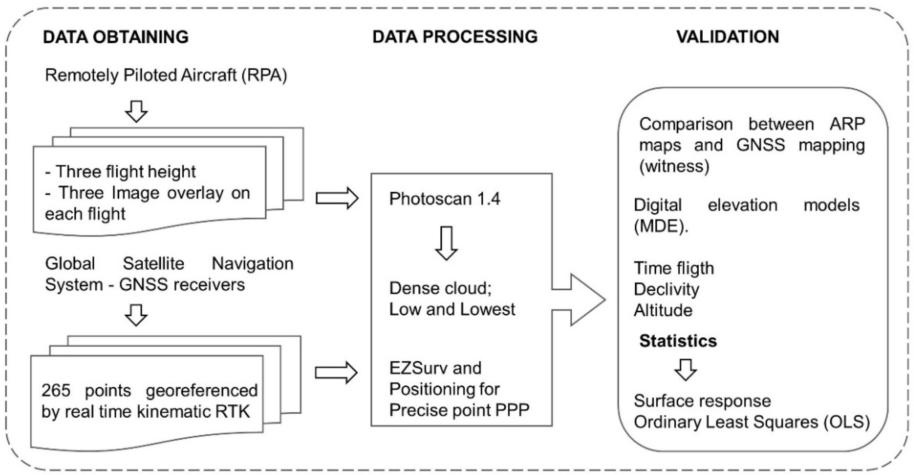
2. Materials and Methods

2.1. Study Area

The study region encompasses an area of eight hectares for coffee cultivation (Figure 1). It is located in Bom Sucesso, Minas Gerais, Brazil, at 21°00′55″ S and 44°54′57″ W. The region has a hot and temperate climate, the mean annual temperature is between 20 and 22 °C, the annual rainfall is between 1300 and 1600 mm, and the altitude is between 800 and 1000 m [23].

2.2. Data Collecting and Processing

Photogrammetric and geodesic techniques were performed together. In some analyses, the methodologies may be confused; therefore, the steps for conducting the research are presented in a flowchart in Figure 2.

2.3. Data of GNSS Receivers

A conventional topographic survey method was performed using GNSS receivers. They were operating in real-time kinematic (RTK) mode, consisting of a base and rover with a 0.03 m precision. Spectra Precision equipment model SP60 was used, a receiver of 240 channels at frequencies of C/A, L1, L2 and L3 (Figure 3a), capturing a total of 265 points (Figure 3b).
The data collected by GNSS receivers were processed using EZSurv software and a digital platform of the Brazilian Institute of Geography and Statistics (IBGE). Geographic coordinates (X, Y, and Z) obtained by the equipment installed in the base were adjusted to the digital platform of the IBGE by Precise Point Positioning (PPP). This positioning method applies an orbit and clock correction in GNSS and a position within a global frame of reference anywhere in the world [24].
The coordinates recalculated by PPP were added to the EZSurv software for coordinate adjustment. Then, points reordering in the project was carried out, which consisted of coordinates adjusting according to base, rover, and satellite triangulation. This step eliminates the defective collection signals and aligns them with the new coordinates provided by PPP available in Universal Transverse Mercator (UTM) coordinates.

2.4. Aircraft and Flight Characteristics

Aerial images were obtained by a DJI Phanton 4 advance RPA (Figure 4) with a RGB sensor with a 1” focal aperture to capture photos of up to 20 megapixels and a spatial resolution of 12 mm to 120 m from the target.
Flight planning began with area delineation and the definition of take-off points. Before starting the flight, some safety factors were observed, including climatic conditions, wind speed, presence of objects, poles, trees, and electrical transmission towers [25]. Next, nine flight missions were planned in the Drone Deploy software under different configurations: AGL at 90, 120, and 150 m and overlapping images: 70% × 70%, 80% × 80%, and 90% × 90%, which were performed in two replicates totalling 18 flights.
The images collected were processed in Agisoft PhotoScan software, version 1.4.3., which is based on the SfM algorithm. SfM approaches can be considered superior to other approaches in terms of accuracy when the user intends to generate orthomosaics and DTMs [26,27].

2.5. Photogrammetric Processing

The methodology used to process the images involved a four-step process, as described by Flynn and Chapra [28] and Rusnák et al. [29]. Step 1: image aligned, phototriangulation process implemented, and a sparse point cloud was generated. Step 2: a sparse point cloud, densification, and detailed representation of the mapped area were developed. Step 3: the dense point cloud and accurate representation of the three-dimensional mapped terrain, DSM, were constructed. Step 4: texture was applied to the DSM model, and a DTM was created and classified into five categories: very high, high, medium, low, and lowest.
Given the large number of points filtered by the SfM, the DEMs use a reduced point mesh. Photogrammetric products are obtained by various processes, which can involve hours of processing, and processing time can be reduced based on the selection of some parameters. Therefore, to increase flight efficiency and maintain design accuracy, different processing combinations were used (Table 1).

2.6. Validation

The reports obtained after data processing were compiled and analysed. In this stage, the processing time for each combination and the accuracy errors generated in orthomosaic formation were considered. Each processing time (combination) was analysed statistically in OriginPRO17 software and represented as a response surface: axis (X), flight height; axis (Y), image overlap; and response axis (Z), processing time. This analysis offers the user a mechanism for predicting the processing time through an equation. Response surface methodology (RSM) is one of the most commonly used multivariate techniques for process optimization and is particularly effective for multivariate systems [30]. By fitting a polynomial model to the experimental data, it was possible to predict the response for all possible factor combinations for the chosen experimental group [31] and a regression model was used to optimize the output variable influenced by the independent variables [32].
The DTMs obtained by photogrammetric (RPA) and geodesic (GNSS) surveys were evaluated using ArcGIS 10.4 software. The data from the properly processed GNSS receivers were considered the control because their data were highly reliable (0.03 m).
The digital models were compared using ordinary least squares (OLS) functions using Spearman’s classification. For this comparison, it was necessary to extract points from the photogrammetric models in a 2 × 2 m mesh. The Spearman classification assesses whether there is a relationship between two variables and whether this can be described through a monotonic function.
From an estimate of the parameters in a linear regression model, the OLS function minimizes the sum of squares and the differences between the observed responses and the responses predicted by a linear function of the explanatory variables. This can be observed as the sum of the squared vertical distances between each data point in the set and the corresponding point in the regression line [33]. In the OLS equation, the mathematical model is applied to the explanatory variables to better predict the dependent variable. In the regression equation, the dependent variable is always Y, and the explanatory variables are always Xs. Each explanatory variable is associated with a regression coefficient that describes the strength and sign of the relationship between this variable and the dependent variable as shown in Equation (1) [34]:
Y = β0 + β1X1 + β2X2 +… βnXn + e
where:
  • Y: dependent variable;
  • Xn: explanatory variable;
  • βn: coefficient;
  • e: random residual error.
Model confidence can be evaluated based on six rules: (1) the coefficients have the expected signs; (2) there is no redundancy between the explanatory variables; (3) the coefficients are statistically significant; (4) the residuals are normally distributed; (5) there is a strong adjusted R squared value; and (6) the residuals are not spatially correlated [34]. Collinearity among the variables was determined according to the six rules of the OLS model.
DSMs accuracy was evaluated from the mean residual errors at each flight height, across the 36 models obtained by SfM photogrammetric processing and models obtained by GNSS receivers, and the summary of the variables (OLS results).

3. Results and Discussion

3.1. Processing Time

In many cases, data processing time is considered a limiting factor to using technologies in the field. Combinations of overlap, flight height, and parameters were analysed in the software to optimize the time required to obtain photogrammetric data (Figure 5).
In terms of processing time, the 150 m AGL flight missions showed the best results. The three overlap levels evaluated at this flight height showed processing times less than 100 min (Figure 5). The 70 × 70% image overlap for flights at 150 m showed shorter processing times due to the low number of images. These parameters showed the best results without considering image accuracy.
Long image processing times occurred at the 90 m flight height and 90 × 90% overlap, followed by those at the 120 m flight (AGL) and 90 × 90% overlap. Excessive processing times results in some applications being unfeasible; in this case, the variations in the available processors should be considered. In addition, errors at the time of image collection and errors related to hardware may occur; this scenario would require new collection efforts, making information collection even more time-consuming. By evaluating the influence of processing time on RPA images, Torres-Sánchez et al. [35] showed that long processing times can be problematic for operations that require rapid results. In their studies, a reduction in overlap and an increase in flight altitude caused drastic reductions in processing time.
Optimization of processing time is an important factor when using digital models on coffee farms. Farms still face several obstacles regarding data processing. The inclusion of technologies related to production in the field is seen as an application that requires a high investment. Using conventional processors for data processing may facilitate access to and the application of these digital models in coffee growing areas. Cost reductions related to using these technologies must be well-managed and understood; this set of analyses enables the viability of precision agriculture projects [36].
An important factor for optimizing the processing of aerial images is point clouds. As shown in Figure 5, the processing time was affected by the reduction in the point cloud from low to lowest. The overlap of 90 × 90% and an AGL of 90 m resulted in a reduction in processing time from 700 to 200 min. Similar results were found in studies by Dandois et al. [37] who, by evaluating altitude, overlap, and climate conditions in forest structure estimates by RPAs, showed that a reduction in the number of point clouds can be an approach to optimizing processing without reducing the quality of the photogrammetric products.
Time optimization in capturing images contributes to rapid data collection without interfering with the quality of photogrammetric products. Pre-flight planning can be an important tool for data collection optimization. Figure 6 presents a fitted model to estimate the time spent on data collection by RPAs between 90 and 120 m (AGL) and with an overlap of images between 70 and 90%.
Adequately reducing the number of images and refining the flight parameters significantly decreases the software processing time. Determining guidelines for this optimization, particularly in terms of strategies for more efficient image collection, contributes to being able to conduct studies in large areas [38]. In addition, the collection of aerial images in a reduced amount of time results in less interference regarding the difference in luminosity and provides more accurate DTMs [39].

3.2. SfM Processing Accuracy

Presenting the errors that occur during image processing makes the discussion about flight efficiency more comprehensive. The errors caused during image processing are shown in Table 2. These errors are linked to the difficulty the software had in processing the images; these errors may be related to noise, poorly sized overlaps, and incorrect image georeferencing.
The best results occurred with the overlap of 90 × 90% (Table 2); however, there is a contradiction because the flights with the 90 × 90% overlap had high processing times due to the amount of information. The best accuracy occurred with the overlap of 70 × 70% and the 150 m flight heights, and this value, outside the expected range, is associated with the stable conditions of the RPAs at the time of their flights. Even with a high level of accuracy, the flight at 150 m AGL and a 70 × 70% overlap had an error in latitude and longitude above 4 m.
Given the errors shown in Table 2, high overlaps and low AGLs contributed to accuracy in the positioning of latitude and longitude. This shows that DEMs from low flight heights can be arbitrarily accurate in their horizontal measurements.

3.3. Precision of Digital Surface Models

The DSMs were evaluated based on the precision level presented at each point compared with that in the model obtained by GNSS. The assumption of normality was verified by applying the residual histogram obtained by the overall mean accuracy for each AGL (Figure 7). In these analyses, the means of all overlaps during each flight were considered. The histogram lines were evaluated according to the similarity between the sides, and biased models have abnormal curves.
It was observed that the data obtained from the 120 m AGL flights corresponded to a data curve closer to a normal distribution, which indicates that it is the best AGL in terms of error distribution. The 90 and 150 m AGL flights showed nonnormally curves in relation to the normal curve. AGLs 90 and 150 m show abnormality about the ideal curve. In AGL 90 m, despite having low residual variation, a group of values reaches residual errors above 0.4 m. This result can be explained by the high level of terrain detail obtained due to the reduced pixel size, leading the algorithm to confuse certain points of the terrain. By evaluating the effects of point density in DTMs, Agüera-Veja et al. [40] reported that high point density implies redundant results and an excessive increase in terrain detail.
The flights at 150 m AGL (Figure 7b) showed variations below 0.4 m, but their data were not consistent. This data composition makes it difficult to understand the errors obtained, thus indicating that flights performed at 150 m AGL had low reliability levels. The uniform distribution of the systematic errors obtained for the 90 m AGL flights did not guarantee that the DTM presented was superior to the others. Stott et al. [41] evaluated the accuracy of DTMs obtained by high-precision RPAs and noted that sets of topographic data derived from SfM may have spatially erroneously distributed complexes, conferring distorted interpretations of the terrain.
The SfM algorithm compensates for the errors due to issues with measuring accuracy by defining how close the measurement is to a reference value. Normally, the algorithm displays the true surface by estimating the mean error value, so the positive and negative deviations can be compensated, preventing a systematic error. The numerical and spatial distributions of errors should also be considered when investigating the quality of the measurement [42].
Errors presented in standard deviations form were obtained by comparing digital models of RPA and receivers GNSS. Figure 8 shows the point errors of each flight height considering the mean values of overlap. In addition, the data presented on the slope map were derived from the model obtained by the GNSS. Positive standard deviation values were found in regions with slopes between 20 and 35%. On steep slopes, the 3D reconstruction algorithm overestimated the slope; and on low slopes, the deviation errors were estimated below the actual position. In regions with steep slopes, Westoby et al. [43] explained that an aerial approach would be particularly advantageous for use on topographically simple terrains, such as flood plains at the bottom of a valley. However, as with stereoscopic reconstruction, steep or almost vertical topography is probably problematic for the SfM technique.
These are important findings when working on a project to create planting rows. The overestimation of sloped regions can identify areas as not suitable for mechanized coffee planting, thus reducing the complete optimization of the area for planting. When obtaining orthomosaics from RGB aerial images, producers and technicians should pay attention to these results and perform an inspection in the field to validate the results. Growing coffee inappropriately on steep slopes causes soil erosion and reduced productivity due to the loss of fertility on the soil surface, resulting in areas of that are of minimal use to a producer [44].
Overestimation of slopes in coffee areas can also be a barrier to mechanized harvesting. Self-propelled harvesters can be regulated according to terrain variations, and some models can be used when there is a 25% inclination. Prior planning of harvest time can be carried out for coffee on slopes. Mechanized harvesting requires 21.6% more time when performed on slopes above 20% than when performed on lower slopes [45]. This demonstrates that of slopes above the normal inclination interfere with other operations in coffee growing areas.
Higher standard deviations occurrence in areas of steep slopes than in other areas was also observed in studies by [46]. Variations were found in the DEM in areas with a high slope gradient and surface roughness. The authors explained the relevance of this finding for geomorphic studies since the processing time is greater for steep slopes. This generates inaccuracies in the models in these locations, causing erroneous interpretations. This scenario can be considered a significant impediment for regions intended for coffee growing since regions with high slopes require specific management, mainly in terms of applying soil conservation and area optimization techniques.
The analyses shown in Figure 8 show the common error between the models. Regions with slopes as high as 15% occur within the error domain, with a standard deviation below the ideal mean. This type of error was found in studies by Lamsters et al. [47], who worked with orthophotos for image reconstruction of glaciers, and the authors observed a constant domain of errors in the flat regions. This type of error was also discussed in the studies by James and Robson [48]; when capturing images in regions with flat topography, the authors observed that the errors in the DTMs were below average. Therefore, for this type of terrain, flights should be conducted by applying slopes to the image capturing sensor.
Despite this type of error, issues with planning and implementing coffee productions in regions considered to have a flat topography are minimal. Even below the ideal altitude, the contour lines considered in this type of project will follow the same direction.
Statistical details of the different combinations of flight configurations are shown in Figure 9. This figure shows the influence of different flight configurations and image processing on topographic quality compared with the classic topography obtained by GNSS receivers. Given this relationship, it is possible to observe in general that the 150 m AGL flights showed the best correlations; but in reviewing the data, we observed that the 120 AGL flight with an 80% overlap resulted in a low processing time and provided the best result.
This result demonstrates that AGL flight height can be configured to make the flight more efficient. In addition, some values found during processing for lowest flights did not differ visually. Therefore, it is possible to reduce processing times while maintaining acceptable levels of accuracy.
The best results shown in Figure 9 are the coefficients observed for the following configurations: 90 m flight, 90 × 90% overlap, and low point density; 120 m flight, 80 × 80% overlap, and low and lowest point densities; and 150 m flight, 80 × 80% overlap, and low and lowest point densities. The comparison of these results with the information related to processing time shows that the 150 m flight with 80 × 80% overlap and a low point density is notable. This flight configuration collects less data and shows significant results in relation to the other configurations. However, when comparing these results with the distribution of errors (Figure 7), the 120 m flights with 80 × 80 overlap and a low point density and those with 80 × 80 overlap and a lowest point density are preferred due to better data uniformity.
Figure 9 highlights an important issue for flight configurations. All flights performed with 80 × 80% overlap, regardless of processing time and flight height, showed a correlation above 98. This overlap is the most appropriate for topographic surveys conducted by using images obtained by RPAs.
Flight optimization should be performed by implementing some processing and precision limits. An increase AGL in flights results in fewer passes over an area, and thus, fewer images are superimposed. Thus, when performing flights in small areas, flight optimization can cause a reduction in the quality of photogrammetric products. James and Robson [38] highlighted the number of images in certain regions and note that the heterogeneity of some areas can decrease and increase errors when fewer images are collected. Thus, the authors recommend capturing at least three images of an area of interest.
This information may be valid for coffee growing projects in small areas. In many countries, especially in globally relevant coffee producing regions, such as South American countries, farms used for coffee plantations are less than 2 hectares (Jha et al., 2011). In these cases, image capture can be configured by increasing the overlap area, reducing the flight speed, and obtaining at least three images per area.
In a discussion on image number, Piermattein et al. [49] highlighted that high numbers of images provide more detailed DEMs. This assumption can be variable and depends on the type of product obtained. As seen in the results presented in Table 2, the increase in the number of images did not show linear significance. The 90 × 90 overlaps added a high level of detail to the DEMs, and when compared with traditional topographic methods, these overlap levels were considered inferior. High levels of detail combined with an altitude reduction were reported by Avtar et al. [50], who evaluated different flight heights for biophysical analysis of palm trees, and the authors observed a significant contribution of lower altitudes to an increase in errors. This result was attributed to the high level of detail in the image.
The workflow required when processing images involves specific processing steps for objects with high levels of detail. These steps are not necessary for generating DTMs that are applied in agriculture because these steps can significantly increase topographic detail and have relatively high processing times [51]. Photogrammetric products generation requires specific knowledge regarding the type of information that needs to be obtained. Recurring errors occur during data collection, and the increase in the number of images needed to improve the accuracy of a DTM is the main error observed in some cases. According to Micheletti et al. [52], the increase in the number of images collected does not linearly increase DTMs accuracy and may lead to an unnecessary increase in data processing time.
Cartographic data-obtained DTMs are necessary for suitable planting arrangements and soil management for conservation for coffee growing projects. However, the high amount of topographic detail in many cases is unnecessary for coffee growing projects since the recommended commercial spacing between rows is above 3.5 m. What is essential for implementing the coffee growing project is a reliable determination of sloped regions, as this directly interferes with mechanized equipment. Tavares et al. [53] found a direct effect of the slope in coffee growing areas on the mechanized operational field capacity. They showed the operational field capacity decreased harvesting activities of sweeping coffee at slopes above 15%.
Planning and optimization of the image acquisition protocols is challenging in complex natural terrain [54]. Flights optimization in coffee growing projects is valid, and some points should be emphasized. As noted, regions with slopes above 20% are overestimated. In areas with this characteristic, control points on the soil are necessary, which reduces error levels to the geodetic precision level in [55]. It is important to consider the overestimated errors, as this can lead to a reduction in areas suitable for mechanized planting. Höfig and Araújo-Junior [56] showed the ability to mechanize coffee plants in sloping regions. Their research showed that mechanization on slopes of 0–5% is extremely recommended, on slopes of 5.1–10% is very recommended, on slopes of 10.1–15% is recommended, on slopes of 15.1–20% is moderately recommended, and on slopes above 20% is not recommended. Given this assertion, one can consider digital models derived from photogrammetric processes capable of generating a slope map for use in mechanized coffee growing projects.
Cartographic projects for coffee growing from DTMs derived from photogrammetric techniques can be an important tool and contribute to operational improvements. However, it is notable that areas with greater than a 20% slope can show slope values above the actual measurements.

4. Conclusions

The most accurate DTM was derived from the photogrammetric products from the 120 m AGL flight, with frontal and lateral overlap of 80 × 80%. The reduction in image overlap was significant in reducing processing time without influencing the quality of the DTMs.
Images processing in lowest point clouds did not affect the quality of the DTMs. In addition, there was a considerable reduction in processing time.
Slope mapping obtained by ARPs was considered efficient up to a 20% slope, above which the models overestimated the elevation. A dominant error effect was observed in regions with low slopes, usually in photogrammetric constructions that did not use control points in the soil.

Author Contributions

Conceptualization, L.S.S. and G.A.e.S.F.; methodology, M.S.S. and R.d.O.F.; software, D.B.M.; validation, L.S.S., G.A.e.S.F. and R.d.O.F.; formal analysis, D.B.M. and G.R.; investigation, M.S.S.; resources, E.P.; data curation, L.S.S., R.d.O.F. and M.S.S.; writing—original draft preparation, L.S.S.; writing—review and editing, G.A.e.S.F. and L.S.S.; visualization, G.R.; supervision, D.B.M. and E.P.; project administration, G.A.e.S.F.; funding acquisition, G.R. and E.P. All authors have read and agreed to the published version of the manuscript.

Funding

This research was funded by the Embrapa Café—Coffee Research Consortium, project approved No 234/2019.

Institutional Review Board Statement

Not applicable.

Informed Consent Statement

Not applicable.

Acknowledgments

The authors would like to thank farm Bom Jardim, the National Council for Scientific and Technological Development (CNPq), the Coordination for the Improvement of Higher Education Personnel (CAPES) and the Federal University of Lavras (UFLA), the Embrapa Café—Coffee Research Consortium and University of Firenze (UniFI).

Conflicts of Interest

The authors declare no conflict of interest.

References

  1. Belan, L.L.; de Junior, W.C.J.; Souza, A.F.; Zambolim, L.; Filho, J.C.; Barbosa, D.H.S.G.; Moraes, W.B. Management of coffee leaf rust in Coffea canephora based on disease monitoring reduces fungicide use and management cost. Eur. J. Plant Pathol. 2020, 156, 683–694. [Google Scholar] [CrossRef]
  2. de Barbosa, I.P.; Oliveira, A.C.B.; Rosado, R.D.S.; Sakiyama, N.S.; Cruz, C.D.; Pereira, A.A. Sensory quality of coffea arabica l. Genotypes influenced by postharvest processing. Crop Breed. Appl. Biotechnol. 2019, 19, 428–435. [Google Scholar] [CrossRef] [Green Version]
  3. Barbosa, B.D.S.; Ferraz, G.A.E.S.; Santos, L.M.; Santana, L.S.; Marin, D.B.; Rossi, G.; Conti, L. Application of rgb images obtained by uav in coffee farming. Remote Sens. 2021, 13, 2397. [Google Scholar] [CrossRef]
  4. Paccioretti, P.; Córdoba, M.; Balzarini, M. FastMapping: Software to create field maps and identify management zones in precision agriculture. Comput. Electron. Agric. 2020, 175, 105–556. [Google Scholar] [CrossRef]
  5. Yost, M.A.; Kitchen, N.R.; Sudduth, K.A.; Massey, R.E.; Sadler, E.J.; Drummond, S.T.; Volkmann, M.R. A long-term precision agriculture system sustains grain profitability. Precis. Agric. 2019, 20, 1177–1198. [Google Scholar] [CrossRef]
  6. Bernardes, T.; Moreira, M.A.; Adami, M.; Rudorff, B.F.T. Physic-environmental diagnosis of coffee crop in the state of Minas Gerais, Brazil. Coffee Sci. 2012, 7, 139–151. [Google Scholar] [CrossRef]
  7. Gimenes, G.R.; Oliveira, R.B.; Silva, A.F.; Reis, L.C.; Reis, T.E.S. Mapping of slopes for the operation of agricultural harvesters in Bandeirantes Municipality (PR). Semin. Agrar. 2017, 38, 97–107. [Google Scholar] [CrossRef] [Green Version]
  8. Mora, O.E.; Chen, J.; Stoiber, P.; Koppanyi, Z.; Pluta, D.; Josenhans, R.; Okubo, M. Accuracy of stockpile estimates using low-cost sUAS photogrammetry. Int. J. Remote Sens. 2020, 41, 4512–4529. [Google Scholar] [CrossRef]
  9. Brunier, G.; Fleury, J.; Anthony, E.J.; Gardel, A.; Dussouillez, P. Close-range airborne Structure-from-Motion Photogrammetry for high-resolution beach morphometric surveys: Examples from an embayed rotating beach. Geomorphology 2016, 261, 76–88. [Google Scholar] [CrossRef]
  10. Resop, J.P.; Lehmann, L.; Cully Hession, W. Drone laser scanning for modeling riverscape topography and vegetation: Comparison with traditional aerial lidar. Drones 2019, 3, 35. [Google Scholar] [CrossRef] [Green Version]
  11. Nemmaoui, A.; Aguilar, F.J.; Aguilar, M.A.; Qin, R. DSM and DTM generation from VHR satellite stereo imagery over plastic covered greenhouse areas. Comput. Electron. Agric. 2019, 164, 104903. [Google Scholar] [CrossRef]
  12. Akturk, E.; Altunel, A.O. Accuracy assesment of a low-cost UAV derived digital elevation model (DEM) in a highly broken and vegetated terrain. Meas. J. Int. Meas. Confed. 2019, 136, 382–386. [Google Scholar] [CrossRef]
  13. Uysal, M.; Toprak, A.S.; Polat, N. DEM generation with UAV Photogrammetry and accuracy analysis in Sahitler hill. Meas. J. Int. Meas. Confed. 2015, 73, 539–543. [Google Scholar] [CrossRef]
  14. Whitehead, K.; Hugenholtz, C.H.; Myshak, S.; Brown, O.; Leclair, A.; Tamminga, A.; Barchyn, T.E.; Moorman, B.; Eaton, B. Remote sensing of the environment with small unmanned aircraft systems (Uass), part 2: Scientific and commercial applications. J. Unmanned Veh. Syst. 2014, 2, 86–102. [Google Scholar] [CrossRef] [Green Version]
  15. Sopchaki, C.H.; da Paz, O.L.S.; de Salles Graça, N.L.S.; Sampaio, T.V.M. Quality assessment in orthomosaics produced from images obtained with unmanned aerial vehicle without the use of support points. RAE GA-O Espac. Geogr. em Anal. 2017, 43, 200–214. [Google Scholar] [CrossRef]
  16. Scott Watson, C.; Kargel, J.S.; Tiruwa, B. Uav-derived himalayan topography: Hazard assessments and comparison with global dem products. Drones 2019, 3, 18. [Google Scholar] [CrossRef] [Green Version]
  17. Marchi, E.C.S.; Campos, K.P.; Corrêa, J.B.D.; Guimarães, R.J.; Souza, C.A.S. Sobrevivência de mudas de cafeeiro produzidas em sacos plásticos e tubetes no sistema convencional e plantio direto, em duas classes de solo. Ceres 2003, 50, 407–416. [Google Scholar]
  18. Gatziolis, D.; Lienard, J.F.; Vogs, A.; Strigul, N.S. 3D tree dimensionality assessment using photogrammetry and small unmanned aerial vehicles. PLoS ONE 2015, 10, e0137765. [Google Scholar] [CrossRef] [PubMed] [Green Version]
  19. James, M.R.; Robson, S.; d’Oleire-Oltmanns, S.; Niethammer, U. Optimising UAV topographic surveys processed with structure-from-motion: Ground control quality, quantity and bundle adjustment. Geomorphology 2017, 280, 51–66. [Google Scholar] [CrossRef] [Green Version]
  20. Santos Santana, L.; Araújo E Silva Ferraz, G.; Bedin Marin, D.; Dienevam Souza Barbosa, B.; Mendes Dos Santos, L.; Ferreira Ponciano Ferraz, P.; Conti, L.; Camiciottoli, S.; Rossi, G. Influence of flight altitude and control points in the georeferencing of images obtained by unmanned aerial vehicle. Eur. J. Remote Sens. 2021, 54, 59–71. [Google Scholar] [CrossRef]
  21. Gomez, C.; Hayakawa, Y.; Obanawa, H. A study of Japanese landscapes using structure from motion derived DSMs and DEMs based on historical aerial photographs: New opportunities for vegetation monitoring and diachronic geomorphology. Geomorphology 2015, 242, 11–20. [Google Scholar] [CrossRef] [Green Version]
  22. Guerra-Hernández, J.; Cosenza, D.N.; Rodriguez, L.C.E.; Silva, M.; Tomé, M.; Díaz-Varela, R.A.; González-Ferreiro, E. Comparison of ALS- and UAV(SfM)-derived high-density point clouds for individual tree detection in Eucalyptus plantations. Int. J. Remote Sens. 2018, 39, 5211–5235. [Google Scholar] [CrossRef]
  23. Alvares, C.A.; Stape, J.L.; Sentelhas, P.C.; Moraes, G.J.L.; Sparovek, G. Köppen’s climate classification map for Brazil. Meteorol. Z. 2013, 22, 711–728. [Google Scholar] [CrossRef]
  24. Grinter, T.; Roberts, C. Precise Point Positioning: Where are we now? In Proceedings of the IGNSS Symposium 2011, Sydney, NSW, Australia, 15–17 November 2011; pp. 1–15. [Google Scholar]
  25. Dos Santos, L.M.; Ferraz, G.A.S.; Andrade, M.T.; Santana, L.S.; de Barbosa, B.D.S.; Maciel, D.A.; Rossi, G. Analysis of flight parameters and georeferencing of images with different control points obtained by RPA. Agron. Res. 2019, 17, 2054–2063. [Google Scholar] [CrossRef]
  26. Sona, G.; Pinto, L.; Pagliari, D.; Passoni, D.; Gini, R. Experimental analysis of different software packages for orientation and digital surface modelling from UAV images. Earth Sci. Inform. 2014, 7, 97–107. [Google Scholar] [CrossRef]
  27. Dietrich, J.T. Riverscape mapping with helicopter-based Structure-from-Motion photogrammetry. Geomorphology 2016, 252, 144–157. [Google Scholar] [CrossRef]
  28. Flynn, K.F.; Chapra, S.C. Remote sensing of submerged aquatic vegetation in a shallow non-turbid river using an unmanned aerial vehicle. Remote Sens. 2014, 6, 12815–12836. [Google Scholar] [CrossRef] [Green Version]
  29. Rusnák, M.; Sládek, J.; Kidová, A.; Lehotský, M. Template for high-resolution river landscape mapping using UAV technology. Meas. J. Int. Meas. Confed. 2018, 115, 139–151. [Google Scholar] [CrossRef]
  30. Nasri, Z.; Mozafari, M. Multivariable statistical analysis and optimization of Iranian heavy crude oil upgrading using microwave technology by response surface methodology (RSM). J. Pet. Sci. Eng. 2018, 161, 427–444. [Google Scholar] [CrossRef]
  31. Bezerra, M.A.; Santelli, R.E.; Oliveira, E.P.; Villar, L.S.; Escaleira, L.A. Response surface methodology (RSM) as a tool for optimization in analytical chemistry. Talanta 2008, 76, 965–977. [Google Scholar] [CrossRef]
  32. Behera, S.K.; Meena, H.; Chakraborty, S.; Meikap, B.C. Application of response surface methodology (RSM) for optimization of leaching parameters for ash reduction from low-grade coal. Int. J. Min. Sci. Technol. 2018, 28, 621–629. [Google Scholar] [CrossRef]
  33. Wei, W.W. Time series analysis. In The Oxford Handbook of Quantitative Methods in Psychology; Oxford University Press: Oxford, UK, 2006; Volume 2. [Google Scholar]
  34. ESRI Regression Analysis Tutorial for ArcGIS 10 2017. Available online: https://desktop.arcgis.com/en/arcmap/10.3/tools/spatial-statistics-toolbox/regression-analysis-basics.htm (accessed on 20 October 2021).
  35. Torres-Sánchez, J.; López-Granados, F.; Borra-Serrano, I.; Manuel Peña, J. Assessing UAV-collected image overlap influence on computation time and digital surface model accuracy in olive orchards. Precis. Agric. 2018, 19, 115–133. [Google Scholar] [CrossRef]
  36. Zanin, A.; Dal Magro, C.B.; Bugalho, D.K.; Morlin, F.; Afonso, P.; Sztando, A. Driving sustainability in dairy farming from a TBL perspective: Insights from a case study in the West Region of Santa Catarina, Brazil. Sustainability 2020, 12, 6038. [Google Scholar] [CrossRef]
  37. Dandois, J.P.; Olano, M.; Ellis, E.C. Optimal altitude, overlap, and weather conditions for computer vision uav estimates of forest structure. Remote Sens. 2015, 7, 13895–13920. [Google Scholar] [CrossRef] [Green Version]
  38. James, M.R.; Robson, S. Straightforward reconstruction of 3D surfaces and topography with a camera: Accuracy and geoscience application. J. Geophys. Res. Earth Surf. 2012, 117, 1–17. [Google Scholar] [CrossRef] [Green Version]
  39. Nex, F.; Remondino, F. UAV for 3D mapping applications: A review. Appl. Geomat. 2014, 6, 1–15. [Google Scholar] [CrossRef]
  40. Agüera-Vega, F.; Agüera-Puntas, M.; Martínez-Carricondo, P.; Mancini, F.; Carvajal, F. Effects of point cloud density, interpolation method and grid size on derived Digital Terrain Model accuracy at micro topography level. Int. J. Remote Sens. 2020, 41, 8281–8299. [Google Scholar] [CrossRef]
  41. Stott, E.; Williams, R.D.; Hoey, T.B. Ground control point distribution for accurate kilometre-scale topographic mapping using an rtk-gnss unmanned aerial vehicle and sfm photogrammetry. Drones 2020, 4, 55. [Google Scholar] [CrossRef]
  42. Smith, M.W.; Carrivick, J.L.; Quincey, D.J. Structure from motion photogrammetry in physical geography. Prog. Phys. Geogr. 2016, 40, 247–275. [Google Scholar] [CrossRef] [Green Version]
  43. Westoby, M.J.; Brasington, J.; Glasser, N.F.; Hambrey, M.J.; Reynolds, J.M. “Structure-from-Motion” photogrammetry: A low-cost, effective tool for geoscience applications. Geomorphology 2012, 179, 300–314. [Google Scholar] [CrossRef] [Green Version]
  44. Iijima, M.; Izumi, Y.; Yuliadi, E.; Sunyoto; Afandi; Utomo, M. Erosion control on a steep sloped coffee field in Indonesia with alley cropping, intercropped vegetables, and no-tillage. Plant Prod. Sci. 2003, 6, 224–229. [Google Scholar] [CrossRef]
  45. Santinato, F.; Silva, R.P.; de Silva, V.A.; Silva, C.D.; de Tavares, T.O. Mechanical Harvesting of Coffee in High Slope. Rev. Caatinga 2016, 29, 685–691. [Google Scholar] [CrossRef] [Green Version]
  46. Hendrickx, H.; Vivero, S.; De Cock, L.; De Wit, B.; De Maeyer, P.; Lambiel, C.; Delaloye, R.; Nyssen, J.; Frankl, A. The reproducibility of SfM algorithms to produce detailed Digital Surface Models: The example of PhotoScan applied to a high-alpine rock glacier. Remote Sens. Lett. 2019, 10, 11–20. [Google Scholar] [CrossRef] [Green Version]
  47. Lamsters, K.; Karušs, J.; Krievāns, M.; Ješkins, J. High-resolution orthophoto map and digital surface models of the largest Argentine Islands (the Antarctic) from unmanned aerial vehicle photogrammetry. J. Maps 2020, 16, 335–347. [Google Scholar] [CrossRef]
  48. James, M.R.; Robson, S. Mitigating systematic error in topographic models derived from UAV and ground-based image networks. Earth Surf. Process. Landf. 2014, 39, 1413–1420. [Google Scholar] [CrossRef] [Green Version]
  49. Piermattei, L.; Carturan, L.; Guarnieri, A. Use of terrestrial photogrammetry based on structure-from-motion for mass balance estimation of a small glacier in the Italian alps. Earth Surf. Process. Landf. 2015, 40, 1791–1802. [Google Scholar] [CrossRef]
  50. Avtar, R.; Suab, S.A.; Syukur, M.S.; Korom, A.; Umarhadi, D.A.; Yunus, A.P. Assessing the influence of UAV altitude on extracted biophysical parameters of young oil palm. Remote Sens. 2020, 12, 3030. [Google Scholar] [CrossRef]
  51. Javernick, L.; Brasington, J.; Caruso, B. Modeling the topography of shallow braided rivers using Structure-from-Motion photogrammetry. Geomorphology 2014, 213, 166–182. [Google Scholar] [CrossRef]
  52. Micheletti, N.; Chandler, J.H.; Lane, S.N. Investigating the geomorphological potential of freely available and accessible structure-from-motion photogrammetry using a smartphone. Earth Surf. Process. Landf. 2015, 40, 473–486. [Google Scholar] [CrossRef] [Green Version]
  53. de Tavares, T.O.; Silva, R.P.; Santinato, F.; Santos, A.F.; Paixao, C.S.S.; de Silva, V.A. Operational performance of the mechanized picking of coffee in four soil slope. Afr. J. Agric. Res. 2016, 11, 4857–4863. [Google Scholar] [CrossRef] [Green Version]
  54. Stumpf, A.; Malet, J.P.; Allemand, P.; Pierrot-Deseilligny, M.; Skupinski, G. Ground-based multi-view photogrammetry for the monitoring of landslide deformation and erosion. Geomorphology 2015, 231, 130–145. [Google Scholar] [CrossRef]
  55. Santana, L.S.; e Silva Ferraz, G.A.; Cunha, J.P.B.; Santana, M.S.; de Faria, R.O.; Marin, D.B.; Rossi, G.; Conti, L.; Vieri, M.; Sarri, D. Monitoring Errors of Semi-Mechanized Coffee Planting by Remotely Piloted Aircraft. Agronomy 2021, 11, 1224. [Google Scholar] [CrossRef]
  56. Höfig, P.; Araujo-Junior, C.F. Classes de declividade do terreno e potencial para no estado do paraná. Coffee Sci. 2015, 10, 195–203. [Google Scholar]
Figure 1. Study area. (a) Aerial image and study area delimitation (red) and (b) digital terrain model (DTM).
Remotesensing 14 00911 g001
Figure 2. Flowchart for obtaining, processing, and analysing the results.
Remotesensing 14 00911 g002
Figure 3. Topographic survey using GNSS receivers. (a) GNSS receivers and (b) location of points obtained via GNSS.
Remotesensing 14 00911 g003
Figure 4. Equipment used for image collection. Remotely piloted aircraft (RPA), a quadcopter type.
Remotesensing 14 00911 g004
Figure 5. Processing time as a function of combinations between flight altitude, image overlap, and software parameters (point cloud: low and lowest).
Remotesensing 14 00911 g005
Figure 6. The model for flight time pre-planning function as image overlay and flight height (AGL).
Remotesensing 14 00911 g006
Figure 7. Residual histogram of errors, (a) 90 m, (b) 120 m, and (c) 150 m AGL.
Remotesensing 14 00911 g007
Figure 8. Standard deviation between the DTMs obtained by the GNSS receptors and RPAs, (a) 90 m, (b) 120 m, and (c) 150 m.
Remotesensing 14 00911 g008
Figure 9. Ordinary least squares (OLS) results for flight heights, overlays and point clouds compared with those obtained through the topographic survey by GNSS receivers. X-axis: Pearson correlation; y-axis: standard deviation in meters. Colour: AGL; figure format: image overlap; and figure size: error.
Remotesensing 14 00911 g009
Table 1. Interactions between flight parameters and variations in dense cloud processing.
N° ProcessingDense CloudOverlap (Front × Side)Above Ground Level (AGL)
1low70 × 70%90 m
2lowest
3low80 × 80%
4lowest
5low90 × 90%
6lowest
7low70 × 70%120 m
8lowest
9low80 × 80%
10lowest
11low90 × 90%
12lowest
13low70 × 70%150 m
14lowest
15low80 × 80%
16lowest
17low90 × 90%
18lowest
Table 2. Errors in meters obtained through processing reports of PhotoScan 1.4 software.
AGLOverlap (%)Latitude (x)Longitude (y)Altitude (Z)Accuracy (m)
90 m70 × 703.152.641.171.27
80 × 803.242.981.150.55
90 × 901.741.440.640.75
120 m70 × 702.932.041.211.71
80 × 804.243.661.421.58
90 × 902.292.040.920.51
150 m70 × 704.464.091.720.37
80 × 805.825.342.140.88
90 × 902.972.691.160.45
Publisher’s Note: MDPI stays neutral with regard to jurisdictional claims in published maps and institutional affiliations.

