
The SST–Wind Causal Relationship during the Development of the IOD in Observations and Model Simulations


1
Key Laboratory of Marine Hazards Forecasting, Ministry of Natural Resources, Hohai University, Nanjing 210098, China
2
College of Oceanography, Hohai University, Nanjing 210098, China
3
Environmental Science and Engineering, University of North British Columbia, Prince George, BC V2N 4Z9, Canada
4
Southern Marine Science and Engineering Guangdong Laboratory (Zhuhai), Zhuhai 519082, China
5
State Key Laboratory of Satellite Ocean Environment Dynamics, Second Institute of Oceanography, Hangzhou 310012, China
*
Author to whom correspondence should be addressed.
Remote Sens. 2022, 14(5), 1064; https://0-doi-org.brum.beds.ac.uk/10.3390/rs14051064
Submission received: 26 January 2022
/
Revised: 14 February 2022
/
Accepted: 14 February 2022
/
Published: 22 February 2022
(This article belongs to the Topic Climate Change and Environmental Sustainability)
Abstract
:In this paper, we employ reanalysis data to systematically investigate the development of the Indian Ocean dipole (IOD), thereby distinguishing the SST–wind causal relationship during IOD development. The results indicate that the variations in sea surface temperature anomalies (SSTA) are particularly important during IOD development. SSTAs over the eastern Indian Ocean (EIO) lead to variations in Sumatran coastal winds and equatorial zonal winds, whereas SSTAs over the western Indian Ocean (WIO) lag behind these variations. On this basis, the Community Earth System Model (CESM) is adopted to examine the influences of different atmospheric physical processes and model resolutions on the simulation of the IOD evolution. For this purpose, four sets of sensitivity experiments are carried out involving two versions of the Community Atmospheric Model (CAM4 or CAM5) and two atmospheric model resolutions (0.9° × 1.25° or 1.9° × 2.5°). The CAM5 simulation experiments better capture the detailed characteristics of IOD development, especially the wind–SST causal relationship, than the CAM4 experiments. Moreover, increasing the resolution of the atmospheric model can effectively reduce the simulation bias, thus benefiting the simulation of the SST–wind relationship.
1. Introduction
The Indian Ocean dipole (IOD) refers to a strong interannual oscillation of the sea surface temperature (SST) in the Indian Ocean (IO). In the positive IOD phase, a negative sea surface temperature anomaly (SSTA) generally occurs near the island of Sumatra (90°E–110°E, 10°S–0°) in the eastern Indian Ocean (EIO), whereas a positive SSTA typically occurs in the western Indian Ocean (WIO) (50°E–70°E, 10°S–10°N); the opposite behaviors are observed in the negative IOD phase [1]. In recent decades, researchers have widely reported that the IOD plays important roles in not only the Asian monsoon but also global climate change. In particular, the extremely strong IOD event observed in 1997, which was accompanied by a strong El Niño event in the same year, led to severe floods along the east coast of Africa and drought disasters surrounding Indonesia [2], accelerating the study of marine and atmospheric climate anomalies in the tropical Indian Ocean (TIO).
The coupling interaction between the SST and wind constitutes the core component of the Bjerknes feedback and therefore plays a critical role in the IOD development process. A positive IOD event is considered as an example here. When a positive IOD event occurs, a cold-water anomaly and southeasterly wind anomalies are encountered along Sumatra and in the southeastern TIO, respectively. These wind anomalies induce upwelling and tilt the thermocline, both of which cool the EIO and suppress atmospheric convection therein. This reduction in deep convection over the EIO raises the sea level pressure, intensifying the initial easterly winds at the surface. In the following months, the eastern cold-water anomaly extends toward the equator along the Indonesian coast and impacts the Walker circulation through the Bjerknes feedback [3,4,5,6]. The abovementioned easterly wind anomalies gradually emerge in the central TIO, and the western TIO gradually warms. Moreover, the southeasterly wind anomalies moving along the Sumatran coast are further strengthened. After the IOD reaches its peak in October, the whole structure rapidly collapses, and negative IOD events usually occur in the following summer and autumn [7].
One notable challenge in explaining the formation of the IOD is the forcing–response relationship between the SST and wind at the earliest stage of IOD development, namely, how the SSTA triggers wind generation or responds to the wind in the first place. This important question has fascinated many researchers and resulted in numerous studies. For example, Cai et al. (2009) [8], Iskandar et al. (2014) [9] and Feng and Duan (2017) [10] reported that the EIO SSTA is closely related to the thermocline fluctuation and vertical motion caused by Kelvin waves, whereas the genesis of easterly wind anomalies also inherently corresponds to the thermocline fluctuation; all of these phenomena involve a series of interactions and feedback processes between the atmosphere and ocean. Lu and Ren (2020) [11] and Zhang et al. (2020) [12] proposed that easterly wind anomalies attributable to changes in the interhemispheric sea level pressure gradient (between (105°E–150°E, 35°S–10°S) and (105°E–140°E, 10°N–30°N)) play an important role in the formation of IOD events. Nevertheless, the identity of the initial triggering signal between the SST and wind during IOD development remains unclear. Accordingly, in this study, we examine the SST–wind relationship at the beginning of IOD development in detail and attempt to detect the initial triggering signal, which serves as a milestone for model comparisons.
With the utilization of fast computational resources, various coupled numerical models have been developed over the past decade. Coupled models can fully consider the interaction (including the air–sea interaction) of different spatial and temporal scales, and ensure the consistency of the energy budget between the two systems [13,14]. Furthermore, global and regional coupled models can better reveal the physical processes related to air–sea interactions. Coupled models have been used in many aspects of research, such as tropical cyclones, hurricanes, water mass genesis, El Niño-Southern Oscillation (ENSO), IOD and so on [13,15,16,17,18,19].
Current state-of-the-art climate models can adequately simulate certain features and behaviors of the IOD, such as its phase locking (the IOD peak always occurs in autumn), asymmetry (i.e., the asymmetry of the SSTA amplitudes between the positive and negative phases of the IOD), and period (the interval between IOD occurrences) (e.g., Yao et al., 2016 [20]; Hua and Yu, 2015 [21]; Wang et al., 2014 [22]). However, large errors still exist between IOD observations and the simulations using current numerical models; these errors manifest mainly via a warming bias throughout the IO in model simulations [23,24]. In addition, the IOD strength in most models is much greater than observed, which is thought to be caused mainly by an overly strong Bjerknes feedback and a poor simulation of the thermocline feedback with these models [20,25]. It is worth investigating the possible factors responsible for these spurious simulation biases among the various physical processes and model configurations that potentially impact IOD simulations. Yao et al. (2016) [20] investigated the effects of atmospheric physical processes and the horizontal resolution of atmospheric models on IOD simulations by using the Community Earth System Model (CESM), which couples the Parallel Ocean Program (POP) and the Community Atmosphere Model (CAM), along with other components. They mainly discussed the features of the IOD, including its period and amplitude, but neglected to address the SST–wind causal relationship during IOD formation. In this work, we expand the study of Yao et al. (2016) [20] and examine the effects of atmospheric physical processes and the atmospheric model resolution via a comparison with observations. Sensitivity experiments with the CESM are conducted for this purpose. Emphasis is placed on the coupling interaction between wind and the SST, as this interaction dominates the IOD variability.
The structure of this paper is as follows: the second section briefly introduces the model structure, experimental design and observation data. The third section describes the relationship between the variations in the observed SST and wind fields in the TIO. The fourth section presents the evolution of simulated IOD events in numerical CESM experiments. The fifth section summarizes and discusses our findings.
2. Materials and Methods
2.1. Experiment
The CESM is a coupled climate model for simulating the Earth’s climate system. Its predecessor is the Community Climate System Model (CCSM), which was created by the National Center for Atmospheric Research (NCAR) in 1983 as a freely available global atmosphere model for use by the broad climate research community. The development of this model into a fully coupled atmosphere–ocean–land–sea ice model began in 1994. At present, the CESM is widely used in climate simulations and achieves accurate representations of ENSO and the IOD.
CESM version 1.2 is adopted in this study. This model contains several modules, including atmosphere, ocean, land, land ice and sea ice modules, which are connected by a coupler (CPL7) [26]. The greatest improvement in the CESM over the previous version (CCSM4) is the application of the latest version of its Community Atmosphere Model (CAM) component, namely, version 5 (CAM5). The older version (CAM4) in CCSM4 adopted parameterization schemes for deep convection, polar filtering, and the polar cloud fraction compared with previous versions and could be run using three different dynamic schemes (a Eulerian spectral scheme, a semi-Lagrangian scheme and a finite volume scheme) with different resolution settings. In contrast to CAM4 in CCSM4, CAM5 in the CESM relies on a new moist turbulence scheme, a new shallow convection scheme, new stratiform microphysical processes, a revised cloud macrophysics scheme and a new three-mode modal aerosol scheme. In addition, although the vertical stratification in CAM4 includes 26 layers, there are 30 layers in CAM5 [26,27,28].
To study the influences of different atmospheric physical processes and model resolutions on IOD development, we design four CESM coupled experiments with different CAM versions (CAM4 or CAM5) and horizontal resolutions of the atmospheric model (0.9° × 1.25° or 1.9° × 2.5°). These four groups of experiments employ POP version 2 (POP2; [29]) and the Community Land Model version 4 (CLM4; [30]); in addition, sea ice is modeled by the Community Ice Code version 4 (CICE4; [31]), and the coupler is CPL7. POP2 solves the 3-D primitive equations for ocean dynamics using the hydrostatic and Boussinesq approximations. The resolution of POP2 in these experiments is 1° × 1° on a Greenland pole grid with 60 levels in the vertical direction. Detailed information of the experiments is provided in Table 1. All the experiments are integrated over 200 years in the present climate state, and the last 50 years are considered for analysis in this work. The simulation performance for the IOD in these four experiments can be found in Yao et al. (2016) [20].
2.2. Observational Data
The Hadley Centre Sea Ice and Sea Surface Temperature (HadISST) is a combination of monthly globally complete fields of SST and sea ice concentration for period from 1871 to present, which are improved on the basis of Global Sea Ice and Sea Surface Temperature (GISST). HadISST temperatures are reconstructed using optimal interpolation technique using both field observations in situ and the International Comprehensive Ocean Atmosphere Data Set (ICOADS). The satellite data were added after the 1980s. The advanced very high-resolution radiometer (AVHRR) data were used instead Along-Track Scanning Radiometer (ATSR) in HadISST because the former have greater coverage and longer record. HadISST compares well with other published SST datasets and have been widely used in climate and oceanic sciences [32,33,34]. The data used in this study is the monthly mean SST with a spatial resolution of 1° × 1° for 1948–2019.
The National Centers for Environmental Prediction (NCEP) and National Center for Atmospheric Research (NCAR) reanalysis dataset uses a state-of-the-art analysis/forecast system to perform data assimilation using past data from 1948 to the present. This reanalysis dataset uses land surface, ship, rawinsonde, pibal, aircraft, satellite and other data. These data were then quality controlled and assimilated with a data assimilation system. The assimilated observations are upper-air rawinsonde observations of temperature, horizontal wind and specific humidity; operational Television Infrared Observation Satellite (TIROS) Operational Vertical Sounder (TOVS) vertical temperature soundings from NOAA polar orbiters over ocean, cloud-tracked winds from geostationary satellites; aircraft observations of wind and temperature, etc. The introduction of satellite data in 1979 resulted in a significant change in the climatology, especially above 200 hPa and south of 50°S, suggesting that the climatology based on the years 1979–present day is most reliable. The sea surface wind field obtained from NCEP/NCAR reanalysis dataset with a resolution of 2.5° × 2.5° for 1948–2019 is used in this study, which has also been widely used in atmospheric and oceanic research [34,35,36,37]
2.3. Methods
Singular value decomposition (SVD) is a numerical technique used to diagonalize matrices in numerical analysis. In this paper, SVD is mainly used to extract the relationship between multiple element fields, detecting the correlation modes of two element fields.
Denoting two matrices by and , with dimensions m × p and p × n, respectively, we can assume m > n. We compute their covariance matrix :
The with dimensions m × n, it can be discomposed by SVD as below:
and are orthonormal matrices, i.e., they satisfy:
where is the identity matrix. The leftmost n columns of contain the n left singular vectors, and then columns of the n right singular vectors. is the spatial mode corresponding to , is the spatial mode corresponding to , the diagonal elements of is singular values γ [38].
3. Observed Evolution of the IOD
3.1. Statistical Analysis of the SST–Wind Causal Relationship
Before examining the SST–wind causal relationship during IOD events in the model simulation experiments, we first examine the acquired observations. Here, an IOD event is defined as the dipole mode index (DMI) in autumn taking a value greater than one standard deviation (STD) of its long-term evolution over three consecutive months. The DMI is defined as the difference in SSTAs between the western pole (10°S–0°, 90–110°E) and the eastern pole (10°S–10°N, 50°E–70°E). A total of 12 IOD events are selected under this criterion from 1948 to 2019, as detailed in Table 2. Figure 1 shows the evolution of the SSTA field (shading, unit: °C) and wind anomalies (vectors) during IOD development (from occurrence to disappearance), obtained by compositing the 12 IOD events listed in Table 1 during the period from 1948 to 2009. These plots help to compare the SSTAs and wind anomalies during each stage of IOD development, allowing the causal relationship between the SSTAs and wind anomalies to be probed. During boreal spring in IOD years, a weak cold SSTA occurs in the EIO (Figure 1a), whereas the warm SSTA observed in the WIO expands (Figure 1c), the easterly anomalies encountered in the TIO and the southeasterly anomalies moving along the Sumatran coast are not notable (Figure 1c). In summer (Figure 1d–f), obvious southeasterly wind anomalies occur along the Sumatran coast, and significant easterly wind anomalies appear along the equator in August. In autumn (Figure 1g–i), when the zonal gradient of the SST reaches its maximum and the entire TIO is controlled by easterly wind anomalies, the IOD reaches its peak, which is accompanied by strong coastal winds near Sumatra. In boreal winter (Figure 1j–l), the cold SSTA in the EIO gradually dissipates, and the warm anomaly in the WIO expands eastward. Consequently, the wind field anomaly slowly weakens, and the dipole mode of the SSTA collapses. Throughout the entire evolution of the IOD, the interactions between the southeasterly wind anomalies moving along the Sumatran coast and the cold SSTAs in the EIO are considered crucial for IOD formation. Under the effect of feedback, subsequent equatorial zonal wind anomalies can further strengthen the east–west SSTA gradient in the TIO [7,39,40].
The SST–wind causal relationship during IOD events can be analyzed with the singular value decomposition (SVD) method. An IOD-like pattern can be found in the second SSTA mode, as shown in Figure 2a, whereas the first SSTA mode is the basin mode, which is not addressed here. Correspondingly, the second mode of the zonal wind anomaly (UA) is characterized by easterly wind anomalies over the entire TIO with the maximum center located at the equator (Figure 2b). In the meridional direction, southerly anomalies (meridional wind anomaly, VA) dominate over the northeastern IO, with the maximum center along the coast of Sumatra (Figure 2c). These results are consistent with the findings of previous studies [41,42,43,44,45].
To further examine the SST–wind relationship, we chose two key areas based on Figure 2 to define two wind indices, namely, the equatorial zonal wind index (ZWI) averaged over 5°S–5°N and 70°E–90°E, which is the same as that considered in Feng and Meyers (2003) [45], and the Sumatra meridional wind index (SMWI) averaged over 10°S–0° and 85°E–105°E (Figure 2b,c).
Figure 3 shows the lead–lag correlations of the DMI against the ZWI and SMWI. As shown in Figure 3a, when the DMI leads the ZWI and SMWI by 1 month, the strongest negative and positive correlation coefficients of –0.57 and 0.51, respectively, arise with a confidence level of 95%. The one-month lead of the DMI suggests the possibility that the former initially triggers the latter, which promotes the formation of the IOD through the Bjerknes feedback mechanism. For example, when a cold anomaly occurs in the EIO, an SST zonal gradient is formed, resulting in southeasterly winds in the EIO, i.e., a positive correlation between the DMI and SMWI. Furthermore, southeasterly winds continue to extend toward the equator, enhancing the easterly wind anomalies and causing a negative correlation between the DMI and ZWI.
Further analysis focuses on examining the relationships between these wind indices and the SSTAs at the two individual poles. As shown in Figure 3b, the SSTA observed in the EIO is positively correlated with the ZWI with a maximum correlation coefficient of 0.35 when the SSTA leads by 2 months, which is significant at a confidence level of 95%. Moreover, there exists a negative correlation between the EIO SSTA and SMWI, with a maximum correlation when the SSTA leads by 2 months. The above analysis indicates that at the early stage of IOD development, the cold SSTA in the EIO is likely to be the first signal to emerge, which triggers wind variation via the Walker circulation. However, in the WIO, we find that the SSTA lags behind the ZWI and SMWI by one month with peak correlation coefficients of –0.39 and 0.43, respectively (Figure 3c). This indicates that the warm WIO SSTA is intensified by wind anomalies induced by the cold EIO SSTA, suggesting a strong air–sea interaction through IOD development via oceanic forcing of the atmosphere and atmospheric feedback over the ocean.
Figure 4 shows the STDs of the EIO SSTA, WIO SSTA, ZWI and SMWI at the IOD maturity stage (from August to December). The EIO SSTA STD peaks in August, followed by the STDs of both the ZWI and the SMWI in October and the WIO SSTA STD in November. Because the STD can characterize the signal intensity, the temporal evolution of the STDs of these indices further suggests a consequential variation in the wind anomalies and SSTA during IOD development; in other words, the EIO SSTA triggers wind anomalies and further induces the variation in the WIO SSTA, which confirms the finding from the above lead–lag correlation analysis. In August and September, the east–west SSTA gradient in the IO is controlled mainly by cooling in the EIO. Due to the cooling of the EIO, deep convection is suppressed, which impacts the Walker circulation; this series of phenomena can generate equatorial zonal winds and Sumatran coastal winds. Subsequently, under the action of winds, the thermocline in the EIO is uplifted to shallow depths, and upwelling cools the EIO. In contrast, in the WIO, the thermocline deepens, and the accumulation of warm water warms the WIO. Moreover, the increase in the east–west SSTA gradient enhances the easterly wind anomalies over the equatorial IO, further warming the WIO.
We also calculate the lead–lag correlations between the SSTA and the above two wind indices; the results are shown in Figure 5. The spatial distributions of the correlation coefficients are similar to those described in the above analyses. The SSTA near the Sumatran coast attains its maximum negative and positive correlations with the ZWI and SMWI, respectively, at a 2-month lead (Figure 5a,d, respectively), suggesting that the wind anomalies during IOD events are initially caused by cooling in the EIO. Furthermore, a significant correlation emerges at a 0-month lead in the WIO when the correlation in the EIO becomes statistically insignificant. When the SSTA lags behind the wind indices by 1 month, the negative correlation between the ZWI and SSTA and the positive correlation between the SMWI and SSTA in the WIO expand and intensify to their peak values (Figure 5c,f, respectively); this behavior sheds light on the important role of equatorial zonal winds in the warming of the WIO through advection. These results are consistent with the role of zonal advection in WIO warming addressed in the literature [46].
3.2. Case Analysis of the SST–Wind Causal Relationship
The aforementioned SST–wind causal relationship is based on an overall statistical analysis. In other words, significant differences in the SST–wind causal relationship may occur among different IOD events. Many previous studies have reported a diversity of dominant factors responsible for IOD development. For example, Endo and Tozuka (2016) [36] discovered varied impacts of ENSO on IOD events. Tanizaki et al. (2017) [47] examined the different contributions of adiabatic vertical mixing and sea surface advection to IOD development. Wang et al. (2016) [42] and Cai et al. (2021) [2] classified different IOD events based on different subsurface temperature variations. Thus, the above composite or statistical analysis is insufficient for a systematic examination of the SST–wind causal relationship. Consequently, for the first time, we next examine the SST–wind relationship for each IOD event during the period of 1948–2019.
To quantify the initial variation in the SST or wind field during an IOD event, we consider both its value and its temporal tendency (. Following the definition of El Niño events, we also consider a three-month running mean. We define the time of the maximum tendency as the timing of an essential variation in this variable toward the development of an IOD event. Using this definition, we detect the calendar month of the initial variation for both SSTAs and wind anomalies, as indicated in Table 2. Among the 12 IOD events during 1948–2019, 8 events satisfied the aforementioned SST–wind relationship (the EIO SSTA triggers wind anomalies and further induces the variation in the WIO SSTA); these events are labeled with ‘Yes’ in Table 2. In contrast, 4 events did not meet the above SST–wind relationship; these events are labeled with ’No’. Further analysis reveals that among the 4 IOD events that did not satisfy the SST–wind relationship, the variation in the WIO SSTA was greater than that in the EIO SSTA in 3 events (red crosses). However, the variation in the EIO SSTA was much higher than that in the WIO SSTA during the 1961 IOD event, and the cause of the SST–wind relationship mismatch in this event remains unclear.
The typical SST–wind relationship of the EIO SSTA triggers wind anomalies and further induces the variation in the WIO SSTA, as characterized in the 8 IOD events listed in Table 2, can suitably capture the physical mechanism of the Bjerknes feedback. However, during the 3 IOD events with a significant SST variation over the WIO (red crosses), warm SSTAs occurred first over the WIO, causing zonal wind anomalies. EIO cooling was not significant in these IOD events, the mechanism of which could therefore be different from that of typical IOD events. Local wind stress anomalies in the WIO and internal ocean waves may play highly important roles in the development of such an IOD [48].
In summary, the above analyses reveal that during IOD development, cold SSTAs first emerge in the EIO, which triggers meridional wind anomalies near the Sumatran coast as oceans force the atmosphere. Then, coastal wind anomalies strengthen the upwelling process, further cooling the EIO SST. Upon cooling of the EIO SST, the Walker circulation near the equatorial IO can be affected, resulting in easterly wind anomalies near the equator that further induce a warming anomaly at the western pole of the IOD.
Interestingly, how the initial cold EIO SSTA triggers an IOD event in the typical SST–wind relationship remains unclear. Generally, the triggering mechanism of IOD events has remained a difficult issue to comprehend, although several hypotheses have been proposed. The initial cold EIO SSTA could be caused by internal oceanic processes, such as the contribution of vertical advection [44,48], by the oceanic response to the anomalous variations in atmospheric pressure over Australia and East Asia, or by a remote forcing originating from the Pacific through suppressed convection and the resultant along-shore winds off the Indonesian coast [49]. Nevertheless, the IOD mechanism of the initial trigger and phase transition is highly complicated and is likely beyond the scope of the current study, so we leave this issue for future studies to resolve. Next, we examine the CESM simulation results of the SST–wind relationship during IOD development.
4. Model-Simulated Evolution of the IOD
The SST–wind causal relationship is crucial for the development of an IOD event. Thus, the IOD phenomenon can be reliably simulated only when numerical model simulations reproduce the SST–wind causal relationship. In the preceding section, we clarified the SST–wind causal relationship via observations. In this section, we examine the wind–SST relationship in four model experiments to explore the possible impacts of atmospheric physical processes and the model resolution on the air–sea interaction during IOD events.
4.1. IOD Intensity
Figure 6 shows the STDs of several indices from the observation data and four experiments. The IOD intensity is overestimated in all experiments compared with the observations, particularly in the CPL5(2°) experiment. Careful comparison reveals that the larger amplitudes of the simulated IOD events agree with the larger variability of the ZWI and SMWI. The IOD intensity that exhibits the best agreement with the observations is simulated in the CPL4(1°), which also achieves the best simulation results for the MWI and SZWI; the opposite behavior is true for the CPL5(2°) experiment. The relationships between the wind indices and IOD intensity are reminiscent of the Bjerknes feedback linking the SST and winds, as has been widely recognized in the literature [2,45].
Figure 6 shows that the IOD events are stronger in the CAM5 simulations than in the CAM4 simulations. This is probably because the warming bias in the EIO is larger in the CAM4 simulation than in the CAM5 simulation and partially reduces the Bjerknes feedback strength [20]. In contrast, improving the resolution of the atmospheric model is helpful to capture the realistic Bjerknes feedback process by reducing the warming bias in the EIO, resulting in an improved simulation of the IOD intensity.
4.2. SST–Wind Relationship in Coupled Experiments
The development and decay of IOD events are inevitably related to the variation in the SST–wind relationship across the basin of the IO, especially in the EIO. Hence, realistically simulating the SST–wind relationship is critical for successfully simulating the IOD.
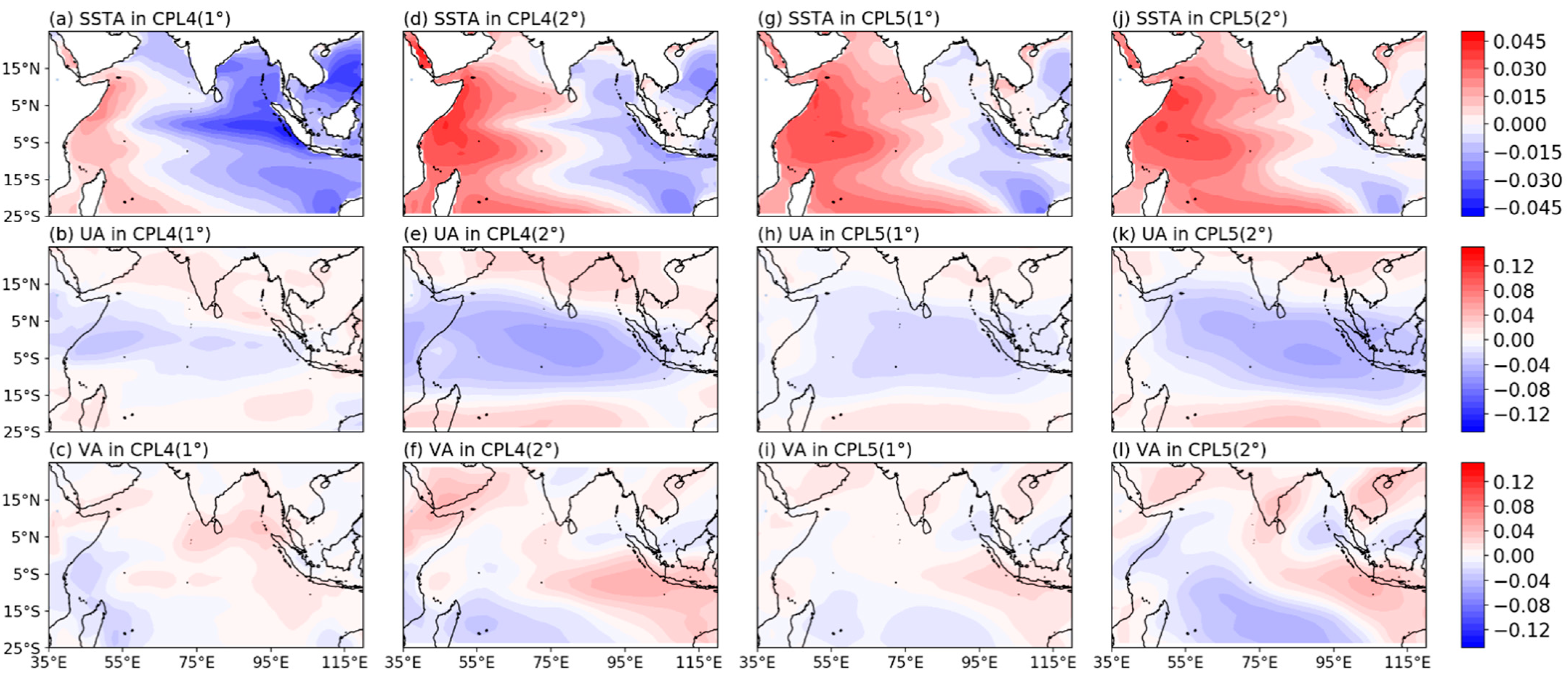
Similar to that derived from the observations, the SST–wind relationship derived from the model experiments can be initially overlooked in SVD analysis. Figure 7 shows the IOD-like patterns obtained with the four models; these patterns account for 21%, 64%, 77% and 66% of the total variance in the CPL4(1°), CPL4(2°), CPL5(1°) and CPL5(2°) experiments, respectively. In the CPL4(1°) experiment, the IOD-related mode yields the smallest variance contribution, and the SST–wind covaried pattern further indicates the largest departure from the observed pattern, as shown in Figure 2, relative to its counterparts in the other three models. The CPL5 experiments seem to capture the covariance center more realistically for the EIO SSTA, especially the CPL5(1°) experiment, whereas the EIO SSTA center is spuriously located around the equator in the CPL4(1°) experiment. Similarly, the covaried structure of winds (zonal and meridional winds) is also more realistically captured in the CPL5 experiments than in the CPL4 experiments based on a comparison with Figure 2. For example, the negative zonal wind anomalies are maximized in the equatorial WIO in the CPL4(1°) experiment rather than in the EIO, as observed.
Similar to the observations, we calculate the lead–lag correlation coefficients between the SSTAs and winds using the EIO SSTA, ZWI, SMWI and WIO SST. Table 3 provides the maximum correlations and corresponding lead–lag times. A negative lead time in the correlation between x and y indicates x leading y, whereas a positive lead time indicates y leading x. As shown in Table 3, the EIO SSTA always leads both the ZWI and the SMWI, whereas the WIO SSTA always lags behind both the SMWI and the ZWI, similar to the observations. This indicates that all models can accurately capture the actual SST–wind causal relationship. However, the intensities of the correlations in the simulations are all much higher than those in the observations, which is attributed to the models containing an overly strong Bjerknes feedback, as mentioned above. In terms of the lead–lag time, the CPL4(1°) experiment seems to provide the worst result, with the EIO SSTA leading the ZWI by 1 month and the WIO SSTA lagging behind the SMWI by 2 months, both of which are quite different from the observations.
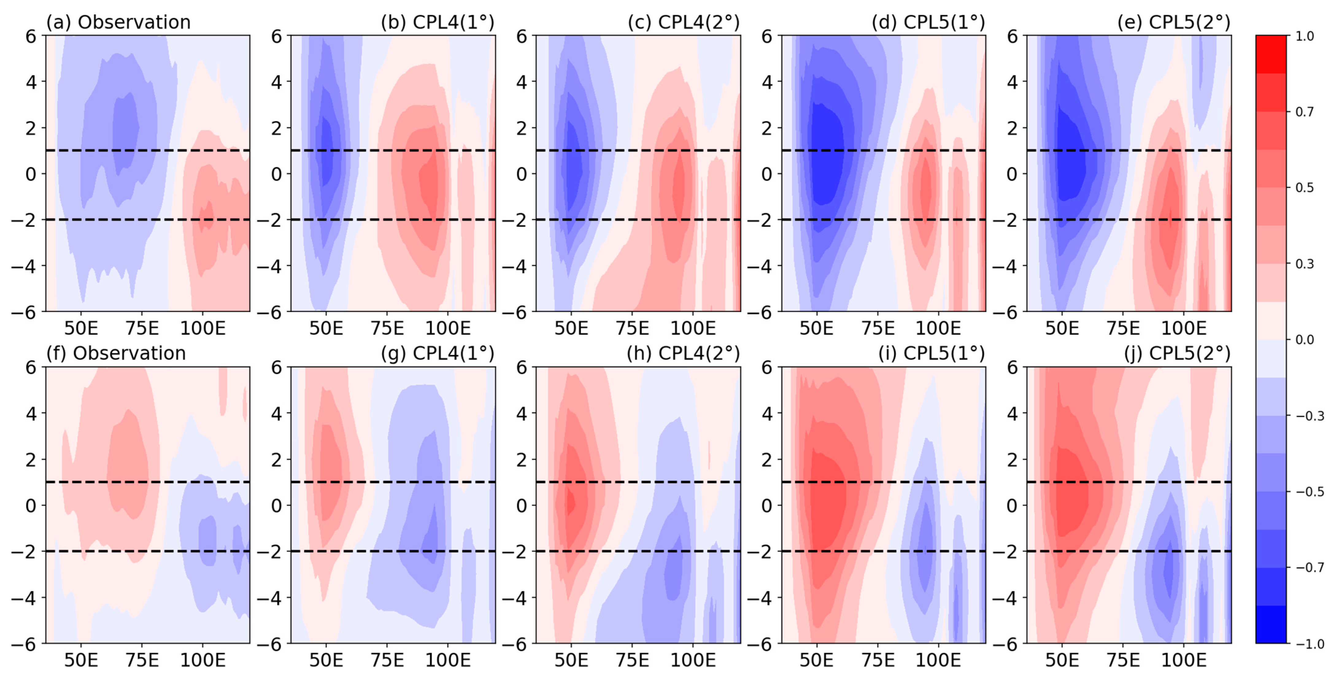
Figure 8 shows longitude diagrams of the lead–lag correlation coefficients between the SSTA and the ZWI and SMWI averaged along the equatorial belt (5°N–5°S). Compared with the observations (Figure 8a,f), all experiments can to a certain extent characterize the actual lead–lag SST–wind relationships. For example, there is a positive correlation in the EIO and a negative correlation in the WIO for the ZWI and vice versa for the SMWI. This outcome indicates that all model settings can suitably capture the Bjerknes feedback. However, there are significant differences in the SST–wind relationship among these experiments. Apparently, the CAM5 experiments yield unrealistically higher correlations than those obtained by the CAM4 experiments, especially in the WIO. This suggests that CAM5 strengthens the Bjerknes feedback, which is particularly pronounced in the equatorial WIO close to the Seychelles–Chagos thermocline ridge. The atmospheric model resolution does not considerably impact the strength of the SST–wind relationship, but a coarse solution yields a longer time lead for the maximum correlation between the EIO SST and winds. For example, the maximum correlation between the EIO SST and ZWI occurs when the SST leads the winds by 1 month in the observations and CPL5(1°) experiment, but the maximum correlation in the CPL5(2°) experiment occurs when the SST leads the ZWI by 2 months. A longer time lag suggests a delayed response of winds to SST variation, probably attributable to the persistently stronger Bjerknes feedback mentioned above. If the simulated SST–wind relationships are ranked in comparison with their observation-based counterparts, the order is CPL5(1°) > CPL4(1°) > CPL5(2°) > CPL4(2°).
As shown in Figure 9, the monthly STDs of the EIO SSTA, WIO SSTA, ZWI and SMWI are used to represent the seasonal variation in the evolution of the IOD in each of the four experiments. The STDs of these four indices are larger in all experiments than in the observations. Additionally, the deviations are larger in the CAM5 experiments, and the higher-resolution experiment can reduce these deviations. However, only the CPL5(1°) experiment can reproduce the lead–lag relationship encountered in the observations, in which the time of the maximum STD of the SSTA and wind indices basically follows the sequence of the EIO SSTA triggers wind anomalies and further induces the variation in the WIO SSTA (as marked with the red stars in Figure 9). The differences between the four experiments are reflected mainly in the simulation results of the wind field. In the CPL4(1°), CPL4(2°) and CPL5(2°) experiments, the SMWI reaches its maximum in December (Figure 9c), which is later than indicated by the observations. Moreover, the time of the maximum variance in the ZWI is inconsistent with that in the observations in the CPL5(2°) and CPL4(1°) experiments. The worst performance is achieved in the CPL4(1°) experiment, indicating that the maximum STDs of the ZWI, SMWI and WIO SSTA occur at the same time. In general, the CPL5(1°) experiment can most accurately simulate the sequence of winds and SST when the IOD is at its peak.
4.3. Simulated SST–Wind Relationships during the Individual IOD Events
In this section, we further examine the SST–wind relationship during each simulated IOD event, similar to the observations. To this end, we first define the IOD events for the models by applying the same IOD definition as applied to the observations. The number of IOD events satisfying the criterion in each of the four experiments is provided in Table 4. In the above analysis of the observations, we reveal that for IOD events with significant WIO SSTA variability, the lead–lag relationship between the SST and winds is quite different from that for IOD events with significant EIO SSTA variability.
Accordingly, a similar case-to-case analysis of the model simulation results is conducted in this subsection. With the same strategy of applying the 3-month running mean of the trend to the observations, we count the number of IOD events satisfying the SST–wind relationship (the EIO SSTA triggers wind anomalies and further induces the variation in the WIO SSTA) in each IOD event, as indicated in Table 4. We find that the typical SST–wind relationship encountered in the observations is not favorable in the simulations, especially in the CPL4 experiments. In the observations, the SST–wind relationship can be classified by the initial variation in the SSTA (either in the EIO or in the WIO), followed by the variation in the winds. However, the SST–wind relationships in the simulations are quite complicated and therefore cannot simply be classified into categories. In addition, the CPL5 experiments yield more realistic SST–wind relationships than the CPL4 experiments, as indicated by the former presenting more events that satisfy the sequence of the EIO SSTA triggers wind anomalies and further induces the variation in the WIO SSTA.
In the observations, we discover that the SST–wind relationship depends on the SSTA variability amplitude in either the EIO or the WIO. Unfortunately, the simulated SSTA variability is always much lower in the WIO than in the EIO, excluding the possibility of using this relative variability to examine the SST–wind relationship in the simulations. Nevertheless, the reason why the WIO SSTA variability is always lower than the EIO SSTA variability remains unclear, probably due to an overly strong Bjerknes feedback in the EIO generating a local enhancement process.
After considering different criteria, we report that the IOD intensity may play an important role in determining the SST–wind relationship. Implementing a classification based on 1.5 times the STD, we count the numbers of both strong and weak events adhering to the sequence of the EIO SSTA triggers wind anomalies and further induces the variation in the WIO SSTA. The results indicate that strong IOD events adhere better to the sequence of the EIO SSTA triggers wind anomalies and further induces the variation in the WIO SSTA, especially in the CPL5 experiments, as revealed in Table 4. Among the strong IOD events in all models, the proportion of events satisfying the sequence of the EIO SSTA triggers wind anomalies and further induces the variation in the WIO SSTA is 19/32 compared with the proportion of 5/16 among the weak IOD events.
In conclusion, the strength of the SST–wind coupling in the IOD simulations is reflected predominantly in the Bjerknes feedback. Hence, in the CAM5 experiments with a stronger Bjerknes feedback, the SST–wind correlation is higher. Moreover, CAM5 improves the simulation of the wind field due to the optimized parameterization [50]; therefore, CAM5 can more accurately capture the sequence of the SST–wind relationship. An improvement in the horizontal resolution of the atmospheric model also contributes to more accurately simulating the IOD development process.
5. Summary and Discussion
The IOD greatly impacts weather and climate anomalies around the world [2,7]. Consequently, it has long been of interest to better understand the IOD and its physical processes to accurately predict IOD events. To this end, a number of IOD mechanism studies have been conducted within the framework of coupled positive and negative feedback loops, among which the wind–SST–thermocline Bjerknes feedback plays a critical role. The importance of SST–wind coupling during IOD development has been widely recognized, but its causality, analogous to the chicken and egg relationship, remains unclear. In this study, we perform a holistic examination of their mutual relationship in observations and model results. Emphasis is placed on identifying the initial trigger in this relationship. The main conclusions can be summarized as below
5.1. Conclusions
In this work, we first conducted comprehensively statistical analyses and case-by-case studies using a long-term observation data to aim at the SST- wind relationship during the IOD development. A causal relationship between SSTA and wind anomalies at the beginning of IOD development is identified for the first time. It was found that the SSTA in the EIO is the first signal to emerge when an IOD event occurs, which further induces wind field anomalies in the IO through the Bjerknes feedback, eventually leading to SSTA variation in the WIO. When there is a negative SSTA in the EIO, local deep convection is suppressed, and the pressure field changes, resulting in wind anomalies. Under the action of wind anomalies, tilting of the thermocline strengthens the SSTA and simultaneously warms the WIO.
Furthermore, we explored the SST–wind relationship in model simulations, revealing that CAM5, which improves the simulation of precipitation and zonal wind, better simulates the SST–wind relationship than CAM4, and improving the resolution can further optimize the simulation results. In CAM5, the lead–lag SST–wind relationship is closer to the observations than that in CAM4, and the causal relationship can be accurately expressed, especially in the CPL5(1°) experiment. However, the SST–wind correlation simulated by CAM5 is too strong, which is related to the excessive strength of the simulated Bjerknes feedback. An increased model resolution could also effectively reduce the simulation bias, improving the simulation of the SST–wind relationship and IOD amplitude.
5.2. Discussion
It has been well recognized that there is covariation between SSTA and wind anomalies during the IOD, but the identity of the initial triggering signal between the SST and wind during IOD development remains unclear. Thus, this work is the first time to identify the sequence of the EIO SSTA triggers wind anomalies and further induces the variation in the WIO SSTA. The causal relationship between SSTA and the equatorial wind is an important step in understanding IOD dynamics and in developing the IOD mechanism, which is still a challenging issue.
In previous model studies, researchers mainly paid attention to the model’s ability in simulating such characteristics of IOD as intensity, phase locking, period, etc. In contrast, this work focuses on the simulation of the causal relationship between SST-wind anomalies during IOD development, and especially addresses the impacts of different atmospheric model physics and model resolutions on this causality between SSTA and wind anomalies.
Several limitations should be noted. First, this study identifies a typical EIO SSTA–wind–WIO SSTA relationship in the observations, clarifying a long-term noteworthy causal relationship between the coupled SST–wind loop. However, certain physical processes remain unclear, e.g., what causes the initial variation in the EIO SSTA, and what physical processes are responsible for IOD events that do not satisfy the typical relationship? These questions are highly challenging to answer and thus should be further examined. One possibility is that the EIO SSTA at the early stage of IOD development is likely to be excited by the propagation of wave signals in the ocean [8,51]. These waves play a vital role, driving not only distant signal transmission but also thermocline depth changes [45,52,53], and both processes trigger SSTA variation in the EIO at the early stage of IOD development due to the relatively shallow mixing layer [52].
Second, negative feedback plays a critical role in the phase transition and termination of IOD events, but it remains uncertain what negative feedback processes and mechanisms dominate IOD development and decay. The most widely accepted hypothesis is that SST cooling in the southeastern IO is prevented through the suppression of upward latent heat fluxes and that the suppression of convective activity increases solar radiation over the southeastern IO. Then, the intense monsoonal forcing weakens southeasterly winds off Sumatra, leading to the rapid termination of IOD events [37,40,43]. However, many details have yet to be discovered.
Third, this study focuses only on the initial trigger of the SSTA–wind relationship; therefore, our findings are far from providing a full understanding of the IOD mechanism, which should inevitably involve a negative feedback process. In addition, we define the time when the trend of each index reaches its maximum value as the time of the initial variation in detecting the SST–wind relationship in each IOD event. This criterion reflects the most significant sequential variation in each index, but this approach may overlook the real occurrence of the initial variation in each index.
Finally, this work explores the influences of different atmospheric physical processes and model resolutions on the IOD simulation results, especially on simulating the SST–wind relationship, through different CESM configurations. However, the physical mechanisms responsible for these influences are not discussed. For instance, what physical processes cause the CAM5 and high-resolution experiments to more realistically simulate the SST–wind relationship, and how is this accomplished? Understanding these aspects is of great significance to improving the simulation of IOD events, which is a highly challenging task in its own right and should be pursued in the near future.
Nevertheless, this work comprehensively examines the SST–wind relationship via both a general statistical analysis and a case study and reports that the typical EIO SSTA–wind–WIO SSTA relationship prevails during IOD development. This is one of the few studies on the notable causal relationship between the coupled SST and wind loop. This study is also the first to investigate the impacts of atmospheric physical processes and model resolution on the simulation of the SST–wind relationship during IOD development. Thus, the findings of this work have theoretical significance in advancing our knowledge of the IOD mechanism and are of practical importance in the operational prediction of IOD enhancement.
Future work should address two basic issues: the physical mechanism of IOD and the accurate simulation of the characteristics of IOD. This paper detected the wind-SST causal relationship, making a big step towards the ultimate goal of IOD dynamical mechanism. However, there is still a long way towards a complete image of IOD mechanism. A critical issue unsolved is the physical process of negative feedback responsible for the IOD phase transition. In terms of IOD simulation, this works only investigates the effects of different atmospheric models and their resolutions on IOD. Many issues remain open, for example, the model systematic biases in IO and the over-strong simulation of IOD intensity in current work. It is critical to address these issues, which should be the focus of future research.
Author Contributions
Conceptualization, Y.X., X.T. and Y.T.; methodology, Y.X., X.T., Y.T. and Y.W.; software, Y.X., Z.Y. and Y.W.; writing—original draft preparation, Y.X.; writing—review and editing, Y.T., X.T. and Y.W. All authors have read and agreed to the published version of the manuscript.
Funding
This study was supported by the National Natural Science Foundation of China (42130409), the Fundamental Research Funds for the Central Universities, Hohai University (B200201048, B210201005, B210201021), and the National Natural Science Foundation of China (42176005, 42176028).
Institutional Review Board Statement
Not applicable.
Informed Consent Statement
Not applicable.
Data Availability Statement
The monthly mean SST was retrieved from the Hadley Centre Sea Ice and Sea Surface Temperature (HadISST) dataset (https://www.metoffice.gov.uk/hadobs/hadisst/data/download.html, accessed on 10 November 2020). The sea surface wind field was obtained from the National Centers for Environmental Prediction (NCEP) reanalysis dataset (https://psl.noaa.gov/data/gridded/data.ncep.reanalysis.surface.html, accessed on 9 October 2020).
Conflicts of Interest
The authors declare no conflict of interest.
References
- Saji, N.H.; Goswami, B.N.; Vinayachandran, P.N.; Yamagata, T. A dipole mode in the tropical Indian Ocean. Nature 1999, 401, 360–363. [Google Scholar] [CrossRef] [PubMed]
- Cai, W.; Yang, K.; Wu, L.; Huang, G.; Santoso, A.; Ng, B.; Wang, G.; Yamagata, T. Opposite response of strong and moderate positive Indian Ocean Dipole to global warming. Nat. Clim. Chang. 2021, 11, 27–32. [Google Scholar] [CrossRef]
- Bjerknes, J. Monthly Weather Reyiew Atmospheric Teleconnections From the Equatorial Pacific. Mon. Weather Rev. 1969, 97, 163–172. [Google Scholar] [CrossRef]
- Wyrtki, K. El Niño—The Dynamic Response of the Equatorial Pacific Oceanto Atmospheric Forcing. J. Phys. Oceanogr. 1975, 5, 572–584. [Google Scholar] [CrossRef]
- Chang, P.; Yamagata, T.; Schopf, P.; Behera, S.K.; Carton, J.; Kessler, W.S.; Meyers, G.; Qu, T.; Schott, F.; Shetye, S.; et al. Climate fluctuations of tropical coupled systems—The role of ocean dynamics. J. Clim. 2006, 19, 5122–5174. [Google Scholar] [CrossRef]
- Xie, S.P. Ocean-atmosphere interaction in the making of the walker circulation and equatorial cold tongue. J. Clim. 1998, 11, 189–201. [Google Scholar] [CrossRef]
- Vinayachandran, P.N.; Saji, N.H.; Yamagata, T. Response of the Equatorial Indian Ocean to an unusual wind event during 1994. Geophys. Res. Lett. 1999, 26, 1613–1616. [Google Scholar] [CrossRef]
- Cai, W.; Pan, A.; Roemmich, D.; Cowan, T.; Guo, X. Argo profiles a rare occurrence of three consecutive positive Indian Ocean Dipole events, 2006–2008. Geophys. Res. Lett. 2009, 36, 2006–2008. [Google Scholar] [CrossRef]
- Iskandar, I.; Mardiansyah, W.; Setiabudidaya, D.; Affandi, A.K.; Syamsuddin, F. Surface and subsurface oceanic variability observed in the eastern equatorial Indian Ocean during three consecutive Indian Ocean dipole events: 2006–2008. AIP Conf. Proc. 2014, 1617, 48–51. [Google Scholar] [CrossRef] [Green Version]
- Feng, R.; Duan, W.S. IOD-related optimal initial errors and optimal precursors for IOD predictions from reanalysis data. Sci. China Earth Sci. 2017, 60, 156–172. [Google Scholar] [CrossRef]
- Lu, B.; Ren, H.L. What Caused the Extreme Indian Ocean Dipole Event in 2019? Geophys. Res. Lett. 2020, 47, e2020GL087768. [Google Scholar] [CrossRef]
- Zhang, L.Y.; Du, Y.; Cai, W.; Chen, Z.; Tozuka, T.; Yu, J.Y. Triggering the Indian Ocean Dipole From the Southern Hemisphere. Geophys. Res. Lett. 2020, 47, e2020GL088648. [Google Scholar] [CrossRef]
- Carniel, S.; Benetazzo, A.; Bonaldo, D.; Falcieri, F.M.; Miglietta, M.M.; Ricchi, A.; Sclavo, M. Scratching beneath the surface while coupling atmosphere, ocean and waves: Analysis of a dense water formation event. Ocean Model. 2016, 101, 101–112. [Google Scholar] [CrossRef]
- Olabarrieta, M.; Warner, J.C.; Armstrong, B.; Zambon, J.B.; He, R. Ocean-atmosphere dynamics during Hurricane Ida and Nor’Ida: An application of the coupled ocean-atmosphere-wave-sediment transport (COAWST) modeling system. Ocean Model. 2012, 43–44, 112–137. [Google Scholar] [CrossRef] [Green Version]
- Warner, J.C.; Armstrong, B.; He, R.; Zambon, J.B. Development of a Coupled Ocean-Atmosphere-Wave-Sediment Transport (COAWST) Modeling System. Ocean Model. 2010, 35, 230–244. [Google Scholar] [CrossRef] [Green Version]
- Zambon, J.B.; He, R.; Warner, J.C. Investigation of hurricane Ivan using the coupled ocean–atmosphere–wave–sediment transport (COAWST) model. Ocean Dyn. 2014, 64, 1535–1554. [Google Scholar] [CrossRef]
- Pokhrel, S.; Chaudhari, H.S.; Saha, S.K.; Dhakate, A.; Yadav, R.K.; Salunke, K.; Mahapatra, S.; Rao, S.A. ENSO, IOD and Indian Summer Monsoon in NCEP climate forecast system. Clim. Dyn. 2012, 39, 2143–2165. [Google Scholar] [CrossRef]
- Yamagata, T.; Behera, S.K.; Luo, J.J.; Masson, S.; Jury, M.R.; Rao, S.A. Coupled ocean-atmosphere variability in the tropical Indian ocean. Geophys. Monogr. Ser. 2004, 147, 189–211. [Google Scholar] [CrossRef]
- Wieners, C.E.; Dijkstra, H.A.; de Ruijter, W.P.M. The interaction between the Western Indian Ocean and ENSO in CESM. Clim. Dyn. 2019, 52, 5153–5172. [Google Scholar] [CrossRef] [Green Version]
- Yao, Z.; Tang, Y.; Chen, D.; Zhou, L.; Li, X.; Lian, T.; Ul Islam, S. Assessment of the simulation of Indian Ocean Dipole in the CESM—Impacts of atmospheric physics and model resolution. J. Adv. Model. Earth Syst. 2016, 8, 1932–1952. [Google Scholar] [CrossRef]
- Hua, L.; Yu, Y. Nonlinear responses of oceanic temperature to wind stress anomalies in tropical pacific and indian oceans: A study based on numerical experiments with an OGCM. J. Meteorol. Res. 2015, 29, 608–626. [Google Scholar] [CrossRef]
- Wang, X.; Wang, C. Different impacts of various El Niño events on the Indian Ocean Dipole. Clim. Dyn. 2014, 42, 991–1005. [Google Scholar] [CrossRef]
- Liu, L.; Xie, S.P.; Zheng, X.T.; Li, T.; Du, Y.; Huang, G.; Yu, W.D. Indian Ocean variability in the CMIP5 multi-model ensemble: The zonal dipole mode. Clim. Dyn. 2014, 43, 1715–1730. [Google Scholar] [CrossRef]
- Feng, R.; Duan, W. Investigating the Initial Errors that Cause Predictability Barriers for Indian Ocean Dipole Events Using CMIP5 Model Outputs. Adv. Atmos. Sci. 2018, 35, 1305–1320. [Google Scholar] [CrossRef]
- Cai, W.; Sullivan, A.; Cowan, T.; Ribbe, J.; Shi, G. Simulation of the Indian Ocean Dipole: A relevant criterion for selecting models for climate projections. Geophys. Res. Lett. 2011, 38, L03704. [Google Scholar] [CrossRef] [Green Version]
- Vertenstein, M.; Bertini, A.; Craig, T.; Edwards, J.; Mai, A.; Schollenberger, J. CESM User’s Guide (CESM1.2 Release Series User’s; National Center for Atmospheric Research: Boulder, CO, USA, 2013; Available online: http://www.cesm.ucar.edu/models/cesm1.2/cesm/doc/usersguide/ug.pdf (accessed on 10 November 2020).
- Neale, R.B.; Chen, C.; Lauritzen, P.H.; Williamson, D.L.; Conley, A.J.; Smith, A.K.; Mills, M.; Morrison, H. Description of the NCAR Community Atmosphere Model (CAM 5.0); Ncar/Tn-464 + Str; National Center for Atmospheric Research: Boulder, CO, USA, 2004; p. 214. Available online: https://www.cesm.ucar.edu/models/cesm1.0/cam/docs/description/cam5_desc.pdf (accessed on 10 November 2020).
- Hurrell, J.W.; Holland, M.M.; Gent, P.R.; Ghan, S.; Kay, J.E.; Kushner, P.J.; Lamarque, J.F.; Large, W.G.; Lawrence, D.; Lindsay, K.; et al. The community earth system model: A framework for collaborative research. Bull. Am. Meteorol. Soc. 2013, 94, 1339–1360. [Google Scholar] [CrossRef]
- Danabasoglu, G.; Bates, S.C.; Briegleb, B.P.; Jayne, S.R.; Jochum, M.; Large, W.G.; Peacock, S.; Yeager, S.G. The CCSM4 ocean component. J. Clim. 2012, 25, 1361–1389. [Google Scholar] [CrossRef] [Green Version]
- Lawrence, D.M.; Oleson, K.W.; Flanner, M.G.; Thornton, P.E.; Swenson, S.C.; Lawrence, P.J.; Zeng, X.; Yang, Z.-L.; Levis, S.; Sakaguchi, K.; et al. Parameterization improvements and functional and structural advances in Version 4 of the Community Land Model. J. Adv. Model. Earth Syst. 2011, 3, M03001. [Google Scholar] [CrossRef]
- Holland, M.M.; Bailey, D.A.; Briegleb, B.P.; Light, B.; Hunke, E. Improved sea ice shortwave radiation physics in CCSM4: The impact of melt ponds and aerosols on Arctic sea ice. J. Clim. 2012, 25, 1413–1430. [Google Scholar] [CrossRef]
- Rayner, N.A.; Parker, D.E.; Horton, E.B.; Folland, C.K.; Alexander, L.V.; Rowell, D.P.; Kent, E.C.; Kaplan, A. Global analyses of sea surface temperature, sea ice, and night marine air temperature since the late nineteenth century. J. Geophys. Res. Atmos. 2003, 108. [Google Scholar] [CrossRef]
- Yan, D.; Kai, L.; Wei, Z.; Wei-Dong, Y. The Kelvin Wave Processes in the Equatorial Indian Ocean during the 2006–2008 IOD Events. Atmos. Ocean. Sci. Lett. 2012, 5, 324–328. [Google Scholar] [CrossRef] [Green Version]
- Endo, S.; Tozuka, T. Two flavors of the Indian Ocean Dipole. Clim. Dyn. 2016, 46, 3371–3385. [Google Scholar] [CrossRef]
- Kalnay, E.; White, G.; Woollen, J.; Chelliah, M.; Fiorino, M.; Kanamitsu, M.; Jenne, R.; Kistler, R.; Saha, S.; Kousky, V.; et al. The NCEP-NCAR 50-year reanalysis: Monthly means CD-ROM and documentation. Bull. Am. Meteorol. Soc. 2001, 2, 247–267. [Google Scholar] [CrossRef]
- Tokinaga, H.; Tanimoto, Y. Seasonal transition of SST anomalies in the tropical Indian Ocean during El Niño and Indian Ocean dipole years. J. Meteorol. Soc. Japan 2004, 82, 1007–1018. [Google Scholar] [CrossRef] [Green Version]
- Yuan, J.P.; Cao, J. North Indian Ocean tropical cyclone activities influenced by the Indian Ocean Dipole mode. Sci. China Earth Sci. 2013, 56, 855–865. [Google Scholar] [CrossRef]
- Andrews, H.; Patterson, C. Singular Value Decomposition (SVD) Image Coding. IEEE Trans. Commun. 1976, 24, 425–432. [Google Scholar] [CrossRef]
- Cai, W.; Cowan, T. Why is the amplitude of the Indian ocean dipole overly large in CMIP3 and CMIP5 climate models? Geophys. Res. Lett. 2013, 40, 1200–1205. [Google Scholar] [CrossRef]
- Schott, F.A.; Xie, S.-P.; McCreary, J.P. Indian Ocean circulation and climate variability. Rev. Geophys. 2009, 47, RG1002. [Google Scholar] [CrossRef]
- Iskandar, I.; McPhaden, M.J. Dynamics of wind-forced intraseasonal zonal current variations in the equatorial Indian Ocean. J. Geophys. Res. Ocean. 2011, 116, C06019. [Google Scholar] [CrossRef] [Green Version]
- Wang, H.; Murtugudde, R.; Kumar, A. Evolution of Indian Ocean dipole and its forcing mechanisms in the absence of ENSO. Clim. Dyn. 2016, 47, 2481–2500. [Google Scholar] [CrossRef]
- Li, T.; Wang, B.; Chang, C.P.; Zhang, Y. A theory for the Indian Ocean dipole-zonal mode. J. Atmos. Sci. 2003, 60, 2119–2135. [Google Scholar] [CrossRef] [Green Version]
- Horii, T.; Hase, H.; Ueki, I.; Masumoto, Y. Oceanic precondition and evolution of the 2006 Indian Ocean dipole. Geophys. Res. Lett. 2008, 35, L03607. [Google Scholar] [CrossRef]
- Feng, M.; Meyers, G. Interannual variability in the tropical Indian Ocean: A two-year time-scale of Indian Ocean Dipole. Deep. Res. Part II Top. Stud. Oceanogr. 2003, 50, 2263–2284. [Google Scholar] [CrossRef] [Green Version]
- Li, T.; Zhang, Y.; Lu, E.; Wang, D. Relative role of dynamic and thermodynamic processes in the development of the Indian Ocean dipole: An OGCM diagnosis. Geophys. Res. Lett. 2002, 29, 2110. [Google Scholar] [CrossRef] [Green Version]
- Tanizaki, C.; Tozuka, T.; Doi, T.; Yamagata, T. Relative importance of the processes contributing to the development of SST anomalies in the eastern pole of the Indian Ocean Dipole and its implication for predictability. Clim. Dyn. 2017, 49, 1289–1304. [Google Scholar] [CrossRef]
- Prasad, T.G.; McClean, J.L. Mechanisms for anomalous warming in the western Indian Ocean during dipole mode events. J. Geophys. Res. Ocean. 2004, 109, C02019. [Google Scholar] [CrossRef]
- Annamalai, H.; Murtugudde, R.; Potemra, J.; Xie, S.P.; Liu, P.; Wang, B. Coupled dynamics over the Indian Ocean: Spring initiation of the Zonal Mode. Deep. Res. Part II Top. Stud. Oceanogr. 2003, 50, 2305–2330. [Google Scholar] [CrossRef] [Green Version]
- Xie, S.; Ma, H.Y.; Boyle, J.S.; Klein, S.A.; Zhang, Y. On the Correspondence between short- and long-time-scale systematic errors in CAM4/CAM5 for the year of tropical convection. J. Clim. 2012, 25, 7937–7955. [Google Scholar] [CrossRef] [Green Version]
- Feng, R.; Duan, W.; Mu, M. Estimating observing locations for advancing beyond the winter predictability barrier of Indian Ocean dipole event predictions. Clim. Dyn. 2017, 48, 1173–1185. [Google Scholar] [CrossRef] [Green Version]
- McPhaden, M.J.; Nagura, M. Indian Ocean dipole interpreted in terms of recharge oscillator theory. Clim. Dyn. 2014, 42, 1569–1586. [Google Scholar] [CrossRef]
- Menezes, V.V.; Vianna, M.L. Quasi-biennial Rossby and Kelvin waves in the South Indian Ocean: Tropical and subtropical modes and the Indian Ocean Dipole. Deep. Res. Part II Top. Stud. Oceanogr. 2019, 166, 43–63. [Google Scholar] [CrossRef]
Figure 1.
Evolution of the SSTA field (shading, unit: °C) and wind anomalies (vectors) during IOD development (from occurrence to disappearance) obtained by compositing 12 IOD events listed in Table 1 during the period from 1948 to 2009, (a–l) represent SSTA and wind anomalies pattern from March to February of the next year, respectively. Hachured regions indicate the areas where the SST anomalies are statistically significant, and only statistically significant wind anomalies are plotted. Statistical significance is tested by evaluating the difference between the composite mean and climatological mean at the 95% confidence level.

Figure 2.
Second singular vectors of (a) SSTA (unit: °C), (b) UA (unit: m/s) and (c) VA (unit: m/s) based on SVD analysis. The black boxes in panel (a) denote the western and eastern poles of the IOD. The green boxes in panels (b,c) denote the regions used to calculate the equatorial zonal wind index and Sumatra meridional wind index. The second singular vector accounts for 7.8% of the total variance. The SVD is jointly conducted by SSTA with UA and VA.

Figure 3.
Lead–lag correlation coefficients of the DMI (a), eastern-pole SSTA (b) and western-pole SSTA (c) with the ZWI (blue lines) and SMWI (red lines). The yellow dotted lines indicate the 95% confidence level.
Figure 3.
Lead–lag correlation coefficients of the DMI (a), eastern-pole SSTA (b) and western-pole SSTA (c) with the ZWI (blue lines) and SMWI (red lines). The yellow dotted lines indicate the 95% confidence level.

Figure 4.
Monthly STDs of the eastern-pole SSTA (unit: °C, light blue), western-pole SSTA (unit: °C, blue), ZWI (unit: m/s, gray), and SMWI (unit: m/s, red). The red stars represent the maximum STD of each index at the IOD maturity stage (August–December).
Figure 4.
Monthly STDs of the eastern-pole SSTA (unit: °C, light blue), western-pole SSTA (unit: °C, blue), ZWI (unit: m/s, gray), and SMWI (unit: m/s, red). The red stars represent the maximum STD of each index at the IOD maturity stage (August–December).

Figure 5.
Spatial distributions of the lead–lag correlation coefficients of the ZWI index against the SSTA (a–c), and that of SMWI index against SSTA (d–f). The lead time in each subpanel indicates the lead–lag time (month); a negative (positive) value indicates the SSTA leading (lagging) the wind index, and 0 indicates both correlated simultaneously.

Figure 6.
STDs of the DMI (unit: °C), SMWI (unit: m/s) and ZWI (unit: m/s) in the four groups of experiments.
Figure 6.
STDs of the DMI (unit: °C), SMWI (unit: m/s) and ZWI (unit: m/s) in the four groups of experiments.

Figure 7.
SSTA dipole mode obtained via SVD analysis and the corresponding UA and VA modes in the CPL4(1°) (a–c), CPL4(2°) (d–f), CPL5(1°) (g–i), and CPL5(2°) (j–l) experiments, where the variance accounted for by each dipole mode is 21%, 64%, 77% and 66% of the total variance, respectively. The unit of SSTA pattern is °C; the unit of UA and VA pattern is m/s.

Figure 8.
Lead time-longitude diagrams of the lead–lag correlation coefficients between the ZWI and SSTA (top row) and between the SMWI and SSTA (bottom row). The correlation is the same as that depicted in Figure 5 but for the meridional mean in the equatorial region (5°N°–5°S). (a,f) show the observations, whereas (b,g), (c,h), (d,i) and (e,j) show the results of the CPL4(1°), CPL4(2°), CPL5(1°), and CPL5(2°) experiments, respectively. The y-axis indicates the lead–lag time (month) of the SSTA relative to the wind index where a negative (positive) value indicates the SSTA leading (lagging) the wind index, and 0 indicates the SST synchronously varying with the wind.

Figure 9.
(a) Monthly STDs of the eastern-pole SSTA (°C), (b) western-pole SSTA (°C), (c) SMWI (m/s) and (d) ZWI (m/s) in the observations (light blue) and four experiments, with the CPL4(1°) in blue, CPL4(2°) in gray, CPL5(1°) in red, and CPL5(2°) in green, respectively. The red stars indicate the maximum STD of each index during the IOD evolution.


Table 1.
Model configuration details in the experiment, where N denotes the number of levels.
| Experiment | Atmospheric Physics Model | Resolution (Atmosphere) | Resolution (Ocean) | Time Period | ||
|---|---|---|---|---|---|---|
| Horizontal | Vertical | Horizontal | Vertical | |||
| CPL4(2°) | CAM4 | 1.9° × 2.5° | 26 | gx1v6 | 60 | 50 years |
| CPL4(1°) | CAM4 | 0.9° × 1.25° | 26 | gx1v6 | 60 | 50 years |
| CPL5(2°) | CAM5 | 1.9° × 2.5° | 30 | gx1v6 | 60 | 50 years |
| CPL5(1°) | CAM5 | 0.9° × 1.25° | 30 | gx1v6 | 60 | 50 years |
Table 2.
SST–wind relationship during each IOD event from 1948 to 2019.
| Year | EIO SST Month | WIO SST Month | SMWI Month | ZWI Month | EIO SST STD(°C) | WIO SST STD(°C) | EIO SST → WIND → WIO SST | IOD Intensity |
|---|---|---|---|---|---|---|---|---|
| 1961 | May | May | July | May | 2.7 | 1.1 | No | 3.0 × STD |
| 1963 | Last December | August | Feb | Feb | 2.1 | 1.3 | Yes | 2.0 × STD |
| 1967 | May | August | June | July | 2.2 | 0.4 | Yes | 1.3 × STD |
| 1972 | March | April | July | July | 1.3 | 2.6 | No | 2.7 × STD |
| 1982 | Last December | December | July | August | 1.6 | 1.4 | Yes | 1.9 × STD |
| 1987 | April | March | June | June | 0.1 | 2.4 | No | 1.5 × STD |
| 1994 | March | August | March | June | 3.2 | 0.6 | Yes | 2.5 × STD |
| 1997 | May | October | May | June | 2.9 | 2.1 | Yes | 3.3 × STD |
| 2006 | June | September | July | July | 2.1 | 0.9 | Yes | 1.7 × STD |
| 2015 | June | March | May | July | 0.3 | 2.3 | No | 1.4 × STD |
| 2018 | April | July | May | July | 1.6 | 1.0 | Yes | 1.8 × STD |
| 2019 | May | August | July | July | 2.8 | 2.1 | Yes | 2.7 × STD |
Table 2 The months shown in the table indicate the time when the trends of the DMI, EIO SSTA, WIO SSTA, ZWI and SMWI reach their own maximum values. The STDs of the eastern-pole and west-ern-pole SSTAs are also shown for each IOD event. These events meeting the aforementioned SST–wind relationship (i.e., the EIO SSTA triggering wind anomalies and further inducing the variation in the WIO SSTA, denoted by EIO SSTA → wind → WIO SSTA in the table) are labeled by ‘Yes’, whereas those events not meeting the SST–wind relationship are labeled by ‘No’. The events in which the WIO SSTA variation was more significant than the EIO SSTA variation are labeled by red. The IOD intensity is also given in the last column in the form of multiples of one STD of DMI.
Table 3.
Lead–lag correlations between the SST and wind indices.
| EIO SSTA and ZWI | EIO SSTA and SMWI | WIO SSTA and ZWI | WIO SSTA and SMWI | |||||
|---|---|---|---|---|---|---|---|---|
| Lead Time | Correlation | Lead Time | Correlation | LEAD TIME | Correlation | Lead Time | Correlation | |
| OBS | −2 | 0.35 | −2 | −0.33 | 1 | −0.44 | 1 | 0.40 |
| CPL4(1°) | −1 | 0.61 | −2 | −0.56 | 1 | −0.63 | 2 | 0.51 |
| CPL4(2°) | −1 | 0.72 | −2 | −0.59 | 1 | −0.70 | 1 | 0.66 |
| CPL5(1°) | −1 | 0.71 | −2 | −0.69 | 1 | −0.87 | 1 | 0.74 |
| CPL5(2°) | −2 | 0.72 | −3 | −0.67 | 1 | −0.82 | 1 | 0.73 |
Table 3 The lead–lag correlation coefficients of the eastern-pole SSTA and western-pole SSTA against the ZWI and SMWI, respectively. Only the maximum correlation coefficient (absolute value) and its corresponding lead times (months) are shown in the table. Negative (positive) values of lead times indicate SSTA leading (lagging) wind, whereas positive values indicate SSTA lagging wind. All the results are statistically significant at the 95% confidence level.
Table 4.
Number of IOD events in each group.
| Experiment | CPL4(1°) | CPL4(2°) | CPL5(1°) | CPL5(2°) | Total | ||||
|---|---|---|---|---|---|---|---|---|---|
| Number | Proportion | Number | Proportion | Number | Proportion | Number | Proportion | ||
| DMI > 1.5 × STD | 7 | 3/7 | 7 | 3/7 | 9 | 6/9 | 9 | 7/9 | 19/32 (59%) |
| DMI < 1.5 × STD | 4 | 2/4 | 6 | 1/6 | 6 | 2/6 | 0 | 5/16 (31%) | |
| Total | 11 | 5 (45%) | 13 | 4 (31%) | 15 | 8 (53%) | 9 | 7 (78%) | |
Table 4 The numbers of strong and weak IOD events in each of the four experiments. DMI > 1.5 × STD indicates strong IOD events, whereas DMI < 1.5 × STD indicates weak IOD events. The proportion of IOD events (in %) satisfying the SST-wind relationship (EIO SST → wind → WIO SST) is also listed.
Publisher’s Note: MDPI stays neutral with regard to jurisdictional claims in published maps and institutional affiliations. |
© 2022 by the authors. Licensee MDPI, Basel, Switzerland. This article is an open access article distributed under the terms and conditions of the Creative Commons Attribution (CC BY) license (https://creativecommons.org/licenses/by/4.0/).
Share and Cite
MDPI and ACS Style
Xiao, Y.; Tang, Y.; Tan, X.; Wu, Y.; Yao, Z. The SST–Wind Causal Relationship during the Development of the IOD in Observations and Model Simulations. Remote Sens. 2022, 14, 1064. https://0-doi-org.brum.beds.ac.uk/10.3390/rs14051064
AMA Style
Xiao Y, Tang Y, Tan X, Wu Y, Yao Z. The SST–Wind Causal Relationship during the Development of the IOD in Observations and Model Simulations. Remote Sensing. 2022; 14(5):1064. https://0-doi-org.brum.beds.ac.uk/10.3390/rs14051064
Chicago/Turabian StyleXiao, Yao, Youmin Tang, Xiaoxiao Tan, Yanling Wu, and Zhixiong Yao. 2022. "The SST–Wind Causal Relationship during the Development of the IOD in Observations and Model Simulations" Remote Sensing 14, no. 5: 1064. https://0-doi-org.brum.beds.ac.uk/10.3390/rs14051064
Note that from the first issue of 2016, this journal uses article numbers instead of page numbers. See further details here.