Article

An Improved Algorithm for the Retrieval of the Antarctic Sea Ice Freeboard and Thickness from ICESat-2 Altimeter Data

1
Chinese Antarctic Center of Surveying and Mapping, Wuhan University, Wuhan 430079, China
2
Land Satellite Remote Sensing Application Center, Ministry of Natural Resources, Beijing 100048, China
3
National Satellite Ocean Application Service, Ministry of Natural Resources, Beijing 100081, China
4
Key Laboratory of Space Ocean Remote Sensing and Application, Ministry of Natural Resources, Beijing 100081, China
5
Key Laboratory for Polar Science of the Ministry of Natural Resources, Polar Research Institute of China, Shanghai 200136, China
*
Author to whom correspondence should be addressed.
Submission received: 8 January 2022 / Revised: 12 February 2022 / Accepted: 18 February 2022 / Published: 22 February 2022

Abstract

:
ICESat-2 altimeter data could be used to estimate sea ice freeboard and thickness values with a higher measuring accuracy than that achievable with data provided by previous altimeter satellites. This study developed an improved algorithm considering variable lead proportions based on the lowest point method to derive the sea surface height for the retrieval of Antarctic sea ice freeboard and thickness values from ICESat-2 ATL-07 data. We first collocated ICESat-2 tracks to corresponding Sentinel-1 SAR images and calculated lead (seawater) proportions along each track to estimate the sea surface height in the Antarctic Ocean. Then, the Antarctic sea ice freeboard and thickness were estimated based on a local sea surface height reference and a static equilibrium equation. Finally, we assessed the accuracy of our improved algorithm and ICESat-2 data product in the retrieval of the Antarctic sea ice thickness by comparing the calculated values to ship-based observational sea ice thickness values acquired during the 35th Chinese Antarctic Research Expedition (CHINARE-35). The results indicate that the Antarctic sea ice freeboard estimated with the improved lowest point method was slightly larger than that estimated with the ICESat-2 data product algorithm. The root mean squared error (RMSE) of the improved lowest point method was 35 cm with the CHINARE-35 measured sea ice thickness, which was smaller than that determined with the ICESat-2 data product algorithm (65 cm). Our improved algorithm could provide more accurate data on the Antarctic sea ice freeboard and thickness, thus supporting Antarctic sea ice monitoring and the evaluation of its change under global effects.

1. Introduction

Antarctic sea ice plays a significant role in the Earth’s system, affecting changes in the global climate and environment [1,2]. The sea ice freeboard and thickness are important parameters reflecting the exchange of mass and energy between the atmosphere and ocean [3,4]. Satellite altimetry has been demonstrated to constitute an effective method of retrieving the sea ice freeboard and thickness at the basin scale [5,6]. Through the application of satellite altimeter data derived from the ICESat and CryoSat-2 [7,8,9,10], researchers have obtained information on Arctic and Antarctic sea ice thickness levels and explored the response of the sea ice thickness to climate change [11,12]. The new-generation altimeter satellite of the ICESat-2 (Ice, Cloud, and Land Elevation Satellite-2) provides a new direction for follow-up research.
The first examination of the Antarctic sea ice freeboard and thickness based on laser satellite altimeter data was conducted in the Weddell Sea, which demonstrated that the ICESat could measure the Antarctic total freeboard and sea ice thickness [13]. Yi et al. [14] proposed the lowest point method to retrieve the sea ice thickness from ICESat altimeter data, and their snow depth assumption was consistent with the sea ice freeboard. The advantages and disadvantages of this algorithm for sea ice thickness retrieval were summarized by Kern et al. [15]. The surface elevation measured by the CryoSat-2 altimeter could also be employed to estimate the sea ice freeboard and then be converted into the sea ice thickness [16]. However, researchers have reported that the Antarctic sea ice freeboard and thickness estimated from ICESat and Cryosat-2 data retain certain errors over ship-based and in situ measurements [17,18,19]. The Cryosat-2 satellite has remained in orbit for more than 10 years, and the observation data quality may thus be affected. ICESat-2 was launched on 15 September 2018 with the scientific objectives of polar land ice elevation and sea ice freeboard measurement at a high accuracy. The ICESat-2 generates six beams divided into 2 × 3 arrays to measure profiles of the surface height, as acquired by the Advanced Topographic Laser Altimeter System (ATLAS), and thus provides the ability to estimate the sea ice freeboard. Compared to ICESat and CryoSat-2 data, ICESat-2 altimeter data achieve a better spatial coverage and a higher elevation accuracy [20,21], which makes these data promising in the sustainable retrieval of the Antarctic sea ice freeboard and thickness.
According to the ICESat-2 algorithm theoretical basis document for sea ice products of ATL-07/ATL-10 data [22], sea ice leads were determined to detect the sea surface height for the retrieval of the sea ice freeboard and thickness (hereafter referred to as the ICESat-2 data product algorithm). The ICESat-2 data product algorithm is divided into two components: the ICESat-2 data product algorithm (single), which obtains the sea surface by one beam of measurement data, and the ICESat-2 data product algorithm (comprehensive), which obtains the sea surface by six beams of satellite data. The principle of the ICESat-2 data product algorithm entails the application of photon emission rates associated with surface reflectance to discriminate leads from sea ice. However, the complex environment of the Antarctic Ocean with variable sea ice conditions could result in lead misclassification with the ICESat-2 data product. Another effective method for sea ice freeboard and thickness retrieval in the Antarctic is the application of the lowest measurement points of a certain percentage along the track to determine the local sea surface height (the lowest point method). The percentage could be obtained from collocated remote sensing images [23]. However, the application of the lowest point method for Antarctic sea ice freeboard and thickness retrieval from ICESat-2 altimeter data requires further evaluation.
There are two objectives of this study: (1) to investigate the accuracy of surface classification (sea ice and lead) provided by the ICESat-2 data product; (2) to develop an improved algorithm for Antarctic sea ice freeboard and thickness retrieval from ICESat-2 altimeter data based on the lowest point method. In the remainder of this paper, the data and methods are first introduced in Section 2. Then, we present and analyze the results of our experiments in Section 3. Section 4 focuses on a discussion of the experimental process. Section 5 outlines the conclusions drawn in this study.

2. Materials and Methods
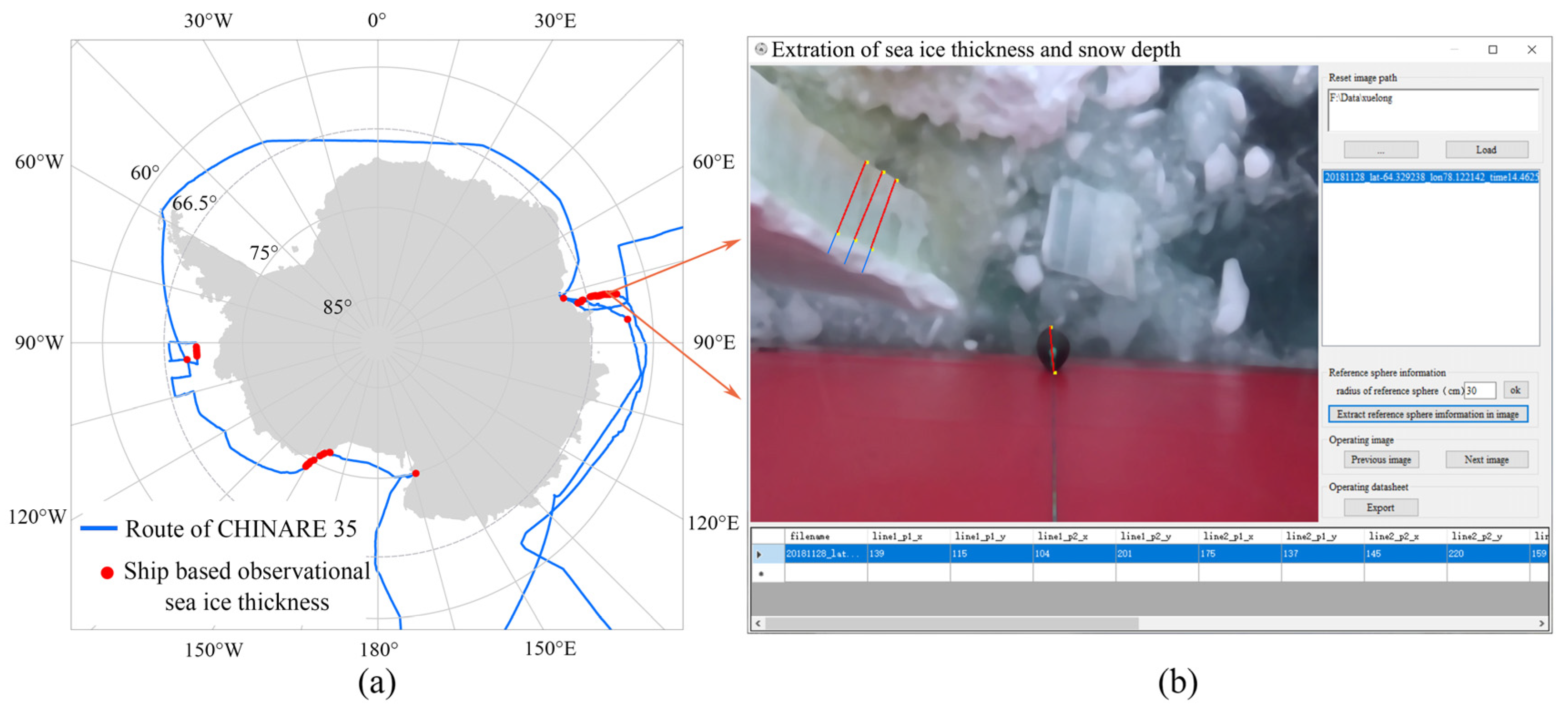
2.1. Study Area

The study area in this paper is the Antarctic Ocean, which consists of five sea areas: the Weddell Sea, the Bellingshausen and Amundsen Sea, the Ross Sea, the Pacific Ocean, and the Indian Ocean (Figure 1). Generally, sea ice in the Antarctic Ocean rapidly shrinks during the melting period, with only the coastal areas of the Antarctic continent remaining, while the opposite occurs during the growth period, in which sea ice rapidly expands away from the shore [24]. Antarctic sea ice is dominated by first-year ice, while a small amount of multiyear sea ice is concentrated in coastal areas [25]. In the Antarctic Ocean, sea ice leads vary with the seasons, which are usually distributed in areas with thin sea ice and are more notably distributed along the coast than in offshore areas [26].

2.2. Data

2.2.1. ICESat-2 ATL-07 and ATL-10 Data

The ICESat-2 exhibits an orbital inclination of 92°, which enables the satellite to detect the region between 88° S and 88° N. The footprint of the ICESat-2 is 17 m, while the segment length of the beams varies from 27 m to 200 m, and the photon elevation accuracy reaches 40 cm [22]. The ICESat-2 altimeter data product provides multiple levels according to the degree of data processing. Among these data, ATL-07 data comprise the ICESat-2 sea ice product containing the surface height and surface type along each of the six ground tracks [21]. ATL-10 data yields the sea ice freeboard derived from ATL-07 data based on a local sea surface reference calculated from the height of the available lead segments. In this study, we used ICESat-2 ATL-07 sea ice height data (November 2018 to October 2019) to estimate the sea ice freeboard based on an improved lowest point (lead) method and then calculated the sea ice thickness according to the static equilibrium equation [13]. ICESat-2 ATL-10 sea ice freeboard data during the same period were also applied to calculate the sea ice thickness. Finally, the sea ice thickness values calculated from the ATL-10-derived sea ice freeboard and ATL-07-derived sea ice freeboard with the improved method in this paper were compared and assessed. We downloaded ICESat-2 ATL-07 and ATL-10 data from the U.S. National Snow and Ice Data Center (NSIDC) (https://nsidc.org/data/ATL07/versions/3, accessed on 7 February 2022; https://nsidc.org/data/ATL10/versions/3, accessed on 7 February 2022) at May, 2020.

2.2.2. AMSR2 Snow Depth Product

The sensor of the Advanced Microwave Scanning Radiometer 2 (AMSR2) is located onboard the Aqua satellite, which was launched on 18 May 2012. The AMSR2 provides accurate measurements of sea ice microwave emissions (brightness temperature), which have been employed to estimate the sea ice concentration and snow depth on sea ice [27,28].
In this study, the AMSR2 snow depth product acquired from the NSIDC (https://nsidc.org/data/AU_SI12/versions/1, accessed on 7 February 2022) was used as input data for sea ice thickness retrieval from ICESat-2 ATL-07 data based on the static equilibrium equation [13]. The NSIDC produces a unified Level 3 snow depth product with a spatial resolution of 12.5 km by applying the snow depth retrieval model proposed by Markus and Cavalieri (1998) [29].

2.2.3. Sentinel-1 and Sentinel-2 Images

Sentinel-1 SAR images exhibit a spatial resolution of 40 m, while the Sentinel-2 optical image spatial resolution is 10 m (Table 1). Since SAR images exhibit a high resolution and can be applied to discriminate leads from sea ice and can monitor sea ice change [30], we used Sentinel-1 images corresponding to ICESat-2 ground tracks with a short time interval (range from 30 to 90 min) to assess the surface type classification provided by the ICESat-2 data product. Sentinel-2 optical images exhibit a higher resolution than that of Sentinel-1 SAR images, meaning that sea ice and leads can usually be identified more accurately. However, Sentinel-2 is a land-observing mission satellite, and its acquisition does not cover as wide an area of the offshore sea ice as Sentinel-1. Considering all of these factors, we obtained Sentinel-1 images to determine the lead location of the sea ice-covered Antarctic Ocean to assess the accuracy of ICESat-2 lead discrimination. Lead proportions were further counted based on Sentinel-1 images with the improved lowest point method to retrieve the Antarctic sea ice thickness from ICESat-2 altimeter data. Sentinel-2 optical images were used in this study to confirm the applicability of Sentinel-1 SAR images. Sentinel-1 and Sentinel-2 images were acquired from https://search.asf.alaska.edu/, accessed on 7 February 2022 and https://earthexplorer.usgs.gov/, accessed on 7 February 2022, respectively.

2.2.4. Ship-Based Observational Sea Ice Thickness Data

In this study, we obtained ship-based observational sea ice thickness data to validate the sea ice thickness data retrieved from the ICESat-2 altimeter. Ship-based observational sea ice thickness data were obtained during the 35th Chinese National Antarctic Research Expedition (CHINARE-35) from November 2018 to January 2019. During CHINARE-35, we used a camera fixed on the side of the scientific expedition vessel (R/V Xuelong) to record sea ice conditions along the ship route. A known-sized reference ball suspended over the side of the ship could be used to estimate the sea ice thickness during the ship’s voyage based on photogrammetric methods (Figure 2). This was accomplished by using the picture to calculate the length ratio of sea ice thickness to a known-length reference bal, and then estimating the sea ice thickness by this ratio. It has been proved that the error of sea ice thickness obtained by this method is less than 7% [31]. These estimates reflected the sea ice thickness along the ship’s route, which could be used in the assessment of the ICESat-2-derived sea ice thickness. Due to environmental factors such as the photography failure during the ship’s voyage and the quality of the photographic images, a total of 1248 measuring points discontinuously distributed across different Antarctic sea areas was finally obtained in this study.

2.3. Methods

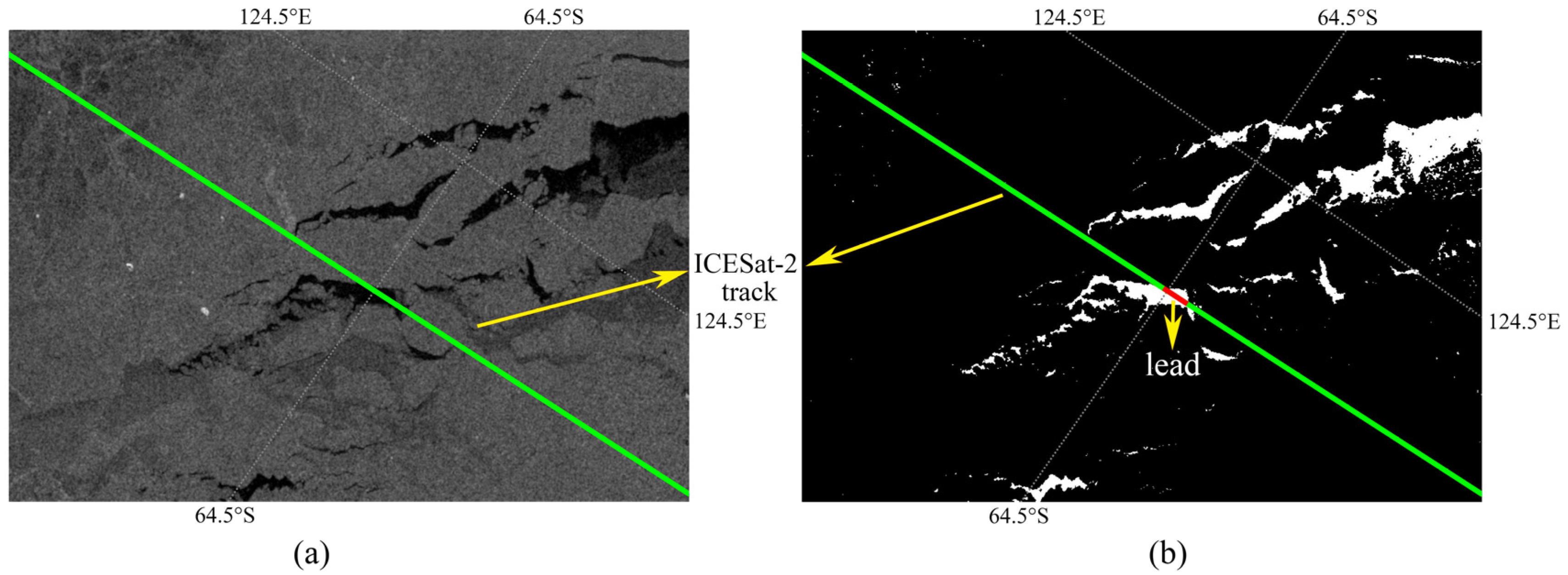
2.3.1. Assessment of Lead Discrimination Based on the ICESat-2 Data Product Algorithm

The ICESat-2 data product provided a surface type (sea ice and lead) classification obtained with a decision tree in the data product algorithm, which was based on the parameters of the photon rate, width of fit, sun elevation angle, and background [32]. Leads with a significantly different reflectance from that of sea ice could be discriminated by a specified reflectance threshold. It should be noted that ICESat-2 measuring points with a high reflectance were considered smooth open-water or thin ice to determine the sea surface height. The ICESat-2 measuring points, which were considered in lead location determination based on ATL-07 data, were flagged as sea surface points in the ICESat-2 data product [32]. A local sea surface reference could then be affirmed by extracting all of the sea surface points and calculating the average height within a certain scope (10-km segments).
Because the local sea surface height (sea ice lead) is an important parameter for the retrieval of the sea ice freeboard and thickness, the classification of the surface type based on ICESat-2 altimeter data is the key step in the accurate retrieval of the sea ice thickness in the Antarctic Ocean. In this study, we extracted sea ice leads from collocated Sentinel-1 images to assess the accuracy of lead discrimination based on the ICESat-2 data product algorithm. In order to ensure the accuracy of the results, we mainly used manual annotation to obtain the lead location.The principles of the selection of Sentinel-1 images are as follows: (1) the leads in Sentinel-1 SAR images should be clearly discriminated where ICESat-2 ATL-07 measuring points are located; (2) the observation time of Sentinel-1 SAR images should match the time of ICESat-2 passage through the same area, aiming to reduce the influence of sea ice drift; and (3) the ground tracks of the ICESat-2 should traverse the lead area in Sentinel-1 SAR images to ensure that lead discrimination with the ICESat-2 algorithm can be assessed. Moreover, Sentinel-2 optical images were obtained to assess the suitability of the selected Sentinel-1 SAR images.

2.3.2. Sea Ice Freeboard and Thickness Retrieval from ICESat-2 Altimeter Data

The sea ice freeboard could be calculated from the local sea surface height based on the ICESat-2 data product algorithm with the lowest point method [13]. In this study, an improved algorithm of the lowest point method with the reflectance sea surface determined by Sentinel-1 images was applied to retrieve the sea ice freeboard and thickness from the ICESat-2 measured surface height data. The process of the improved algorithm derived the sea surface height according to the determined proportion of lowest elevation points as the local sea surface reference. Sea ice and nearby leads could be discriminated via the threshold method because sea ice exhibits a higher reflectivity than that of the leads. Furthermore, the ICESat-2 data product algorithm considered that specular and quasi-specular returns are observed from smooth open water/thin ice surfaces with the ICESat-2, which indicated that high photon rates are expected and that these segments are processed differently [33]. In this study, we explored the acquisition of a local surface height reference by (1) determining the percentage of the lowest elevation points according to the number of leads along ICESat-2 tracks, (2) filtering corresponding measuring points with the reflectivity threshold given by the ICESat-2 data product algorithm, and (3) calculating the local surface height by extracting measuring points using lead proportion.
Since Antarctic sea ice varies over time and space, the traditional lowest point method considering a unique lead proportion for sea ice freeboard and thickness retrieval may generate errors. In this study, we extracted leads from Sentinel-1 images and calculated the percentages of leads along the ICESat-2 track in different months in various Antarctic sea areas. Figure 3 shows an example of an ICESat-2 track crossing a Sentinel-1 SAR image, which was classified through visual interpretation. It should be noted that we used all six beams of the ICESat-2 altimeter data participating in the calculation of the lead proportion for the improved algorithm of the lowest point method. First, the lead proportion along each ICESat-2 track was calculated based on the distribution of pixels representing leads along the whole ICESat-2 track in Sentinel-1 SAR images. Then, we filtered the selected lowest points by the set threshold of the photon rate (lower than 2.5 or higher than 11 for strong beams, while the threshold for weak beams was a quarter of that for strong beams). Finally, the lowest points in each 10-km segment were selected as a local sea surface reference to estimate the sea surface height.
Based on the estimated local sea surface reference, we calculated the 10 km-average height ( h m ) from the surface height ( h o b s ) and then obtained the relative elevation by computing the difference between h and h m . The sea ice freeboard can be calculated as the difference between the relative elevation and the sea surface reference:
h r = h o b s h m    
h f = h r h s s h
where   h r is the relative elevation, h f is the sea ice freeboard, and h s s h   is the sea surface reference height. The specific relationship is shown in the Figure 4. These quantities are both relative to the WGS84 ellipsoid. Finally, the retrieved sea ice freeboard was gridded into 12.5 km × 12.5 km cells.
The sea ice thickness could be calculated from the sea ice freeboard according to the static equilibrium equation [13]. The ICESat-2 is a laser altimeter instrument, which indicates that the sea ice height provided by ICESat-2 ATL-07 data includes the snow depth. We estimated the sea ice thickness ( H i ) through Equation (3) with the input of the sea ice freeboard ( H f ), snow depth ( H s ), snow density ( ρ s ), water density ( ρ w ), and sea ice density ( ρ i ).
H i = ρ w ρ w ρ i H f ρ w ρ s ρ w ρ i H s
In this study, we used   ρ s = 300 km·m-3, ρ w = 1023.9 km·m-3, ρ i = 915.1 km·m-3, and the AMSR2-derived snow depth to calculate the Antarctic sea ice thickness. It should be noted that the sea ice freeboard originated both from the ICESat-2 data product algorithm (ICESat-2 ATL-10 sea ice freeboard) and our improved algorithm of the lowest point method.

3. Results

3.1. Accuracy of Surface Type Classification Based on the ICESat-2 Data Product Algorithm

ICESat-2 ATL-07 data from November 2018 to October 2019 pertaining to the Antarctic were extracted and matched to the collocated Sentinel-1 SAR and Sentinel-2 optical images on the same date. Figure 5 shows the distribution of sea ice and leads in Sentinel-1 SAR images and Sentinel 2 optical images. Sea ice in the red rectangle marked in Figure 4 varied statistically insignificantly in both sets of images (Figure 5a versus Figure 5b, and Figure 5c versus Figure 5d). The overall sea ice conditions changed slightly within a short time, making them suitable for the assessment of labeled lead discrimination based on the ICESat-2 data product algorithm. In addition, a comparison of the Sentinel-1 SAR and Sentinel-2 optical images at a 12-h interval revealed that sea ice slightly drifted under the influence of wind and ocean on the sea ice (Figure 5c and Figure 5d, respectively). These results demonstrated that SAR images with a short time interval could reflect the overall consistent sea ice conditions of the corresponding ICESat-2 data.
Figure 6 shows the error in the ICESat-2-labeled surface type classification with the collocated Sentinel-1 SAR images. The detected misclassification of the surface type with the ICESat-2 data product occurred in two aspects: (1) there were certain points within the leads in the Sentinel-1 images discriminated as sea ice by the ICESat-2 data product algorithm; (2) there occurred points on the sea ice in the images that were identified as leads by the ICESat-2 data product algorithm. Figure 6a,b show that a fair number of points were incorrectly classified over the collocated Sentinel-1 SAR images. Misclassification of the surface type could cause errors in freeboard estimation based on the ICESat-2-measured surface height data. The numerical results of surface type classification from the ICESat-2 ATL-07 data after 2 days indicated that there occurred a large number of lead points misclassified as sea ice by the ICESat-2 data product algorithm (Table 2). The lead discrimination accuracy (defined as the ratio of the number of correct lead classifications to the total number of points labeled as leads in the ICESat-2 data product) ranged from 0% to 42.45%. This could cause errors during subsequent retrieval of the sea ice freeboard and thickness from the ICESat-2 ATL-07 data.

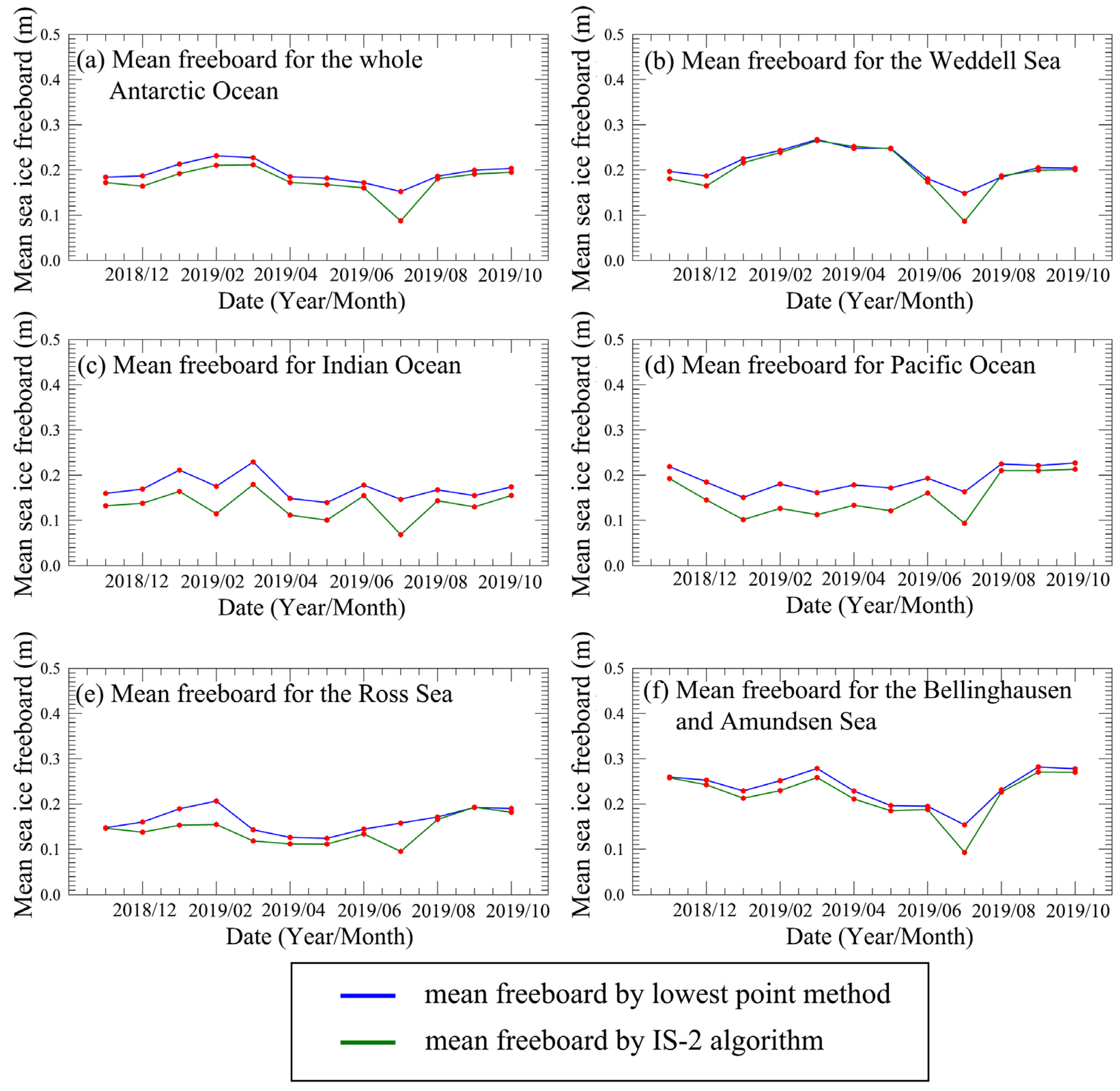
3.2. Antarctic Sea Ice Freeboard Retrieval from ICESat-2 Altimeter Data

Table 3 shows the proportions of leads along the ICESat-2 tracks in the Antarctic Ocean from November 2018 to October 2019 calculated from Sentinel-1 SAR images using the method in Section 2.3.2. It summarizes the proportions of leads during a 12-month period. The lead proportion ranged from 0.73% to 6.67%, and the mean value of the proportion in the different Antarctic Ocean areas ranged from 2.12% to 3.33%, with the maximum and minimum lead proportions observed in the Ross Sea and Indian Ocean, respectively. The lead proportions between November and March were the highest because sea ice in the Antarctic Ocean melted during this period. As Antarctic sea ice increased over time, the lead proportion along the ICESat-2 tracks gradually decreased and then remained stable with the stability of sea ice after March, which is basically consistent with the seasonal process of sea ice variation. The average lead proportion in the Weddell Sea and Indian Ocean was relatively low, while the average proportion in the Ross Sea was the highest. Sea ice in the Ross Sea melted and rapidly drifted, which caused the emergence of numerous leads over the other Antarctic sea areas. Moreover, the sea ice extent in the Ross Sea varied greatly with the season [34], which was consistent with the trends of sea ice motion. Comparatively, sea ice in the Weddell Sea and Indian Ocean melted and drifted relatively slowly because relatively more multiyear ice and fast ice occurred, resulting in a small number of sea ice leads. Previous studies have verified that the area of fast ice in the Indian Ocean is larger than that in the Pacific Ocean [35], which results in a high lead proportion in the Pacific Ocean.
Based on the statistics of the lead proportions along the ICESat-2 tracks in the different months and Antarctic sea areas, we calculated the sea ice freeboard using Equation (1) and Equation (2) while sea surface height was calculated using the improved algorithm (a variable lead proportion value replaced the traditional fixed proportion value) of the lowest point method. The estimated sea ice freeboard was then compared to the sea ice freeboard calculated with the ICESat-2 data product algorithm in the different Antarctic Ocean areas (Figure 7). The Antarctic sea ice freeboard estimated with the improved algorithm of the lowest point method increased by 0.5 cm to 2.2 cm, and the mean value was 1.8 cm larger than the sea ice freeboard estimated with the ICESat-2 data product algorithm. The sea ice freeboard estimates based on the two considered algorithms exhibited earlier increasing and later decreasing trends, with its minimum values occurring in July 2019 in most areas of the Antarctic Ocean. The sea ice freeboard values calculated with the improved algorithm and ICESat-2 data product algorithm were consistent in the Weddell Sea, the Bellingshausen and Amundsen Sea, and the Ross Sea, except in July 2019. The difference was attributed to the lack of ICESat-2 data in early July, which led to the inaccuracy of the ICESat-2 data product algorithm. The difference in the retrieved sea ice freeboard between the ICESat-2 data product algorithm and the improved algorithm in the Indian Ocean and Pacific Ocean was relatively large, probably because these two approaches even behaved differently in regard to fast ice mainly distributed in these two sea areas.

3.3. Spatiotemporal Variations in the Antarctic Sea Ice Thickness from November 2018 to October 2019

The sea ice thickness in the Antarctic Ocean was larger in winter and smaller in summer (Figure 8). The Antarctic sea ice thickness decreased as sea ice melted from November 2018 to January 2019, increased as sea ice grew from February 2019 to July 2019, and then remained stable throughout the rest of the period. Relatively more sea ice, including some multiyear ice, gathered in the Weddell Sea, causing thicker sea ice along the Weddell Sea coast than that in the other Antarctic sea areas. Sea ice in the Bellingshausen and Amundsen Sea, the Indian Ocean, and the Pacific Ocean exhibited the same characteristics of thicker ice concentrated along the coast and thinner ice distributed offshore.
The sea ice thickness in the Weddell Sea was larger than that in the other sea areas in the Antarctic Ocean in summer, with the thickest sea ice distributed in the southwest of the Weddell Sea. Sea ice formed in the east, and eddy currents caused sea ice to accumulate in the western Weddell Sea near the Antarctic Peninsula [36]. A phenomenon occurred in the Ross Sea whereby coastal sea ice was not notably thicker than offshore sea ice, and there occurred almost no sea ice during the sea ice melting period, which was obviously different from the other Antarctic sea areas. Sea ice in the Indian Ocean and Pacific Ocean was dominated by fast ice, which barely drifted, and the sea ice extent was the smallest in the Antarctic Ocean, resulting in a larger value of the spatial average sea ice thickness than that in the other sea areas of the Antarctic Ocean. The sea ice thickness in the Bellingshausen and Amundsen Sea was the second largest, followed by the Weddell Sea, where thicker sea ice was concentrated in the coastal areas throughout the whole year.

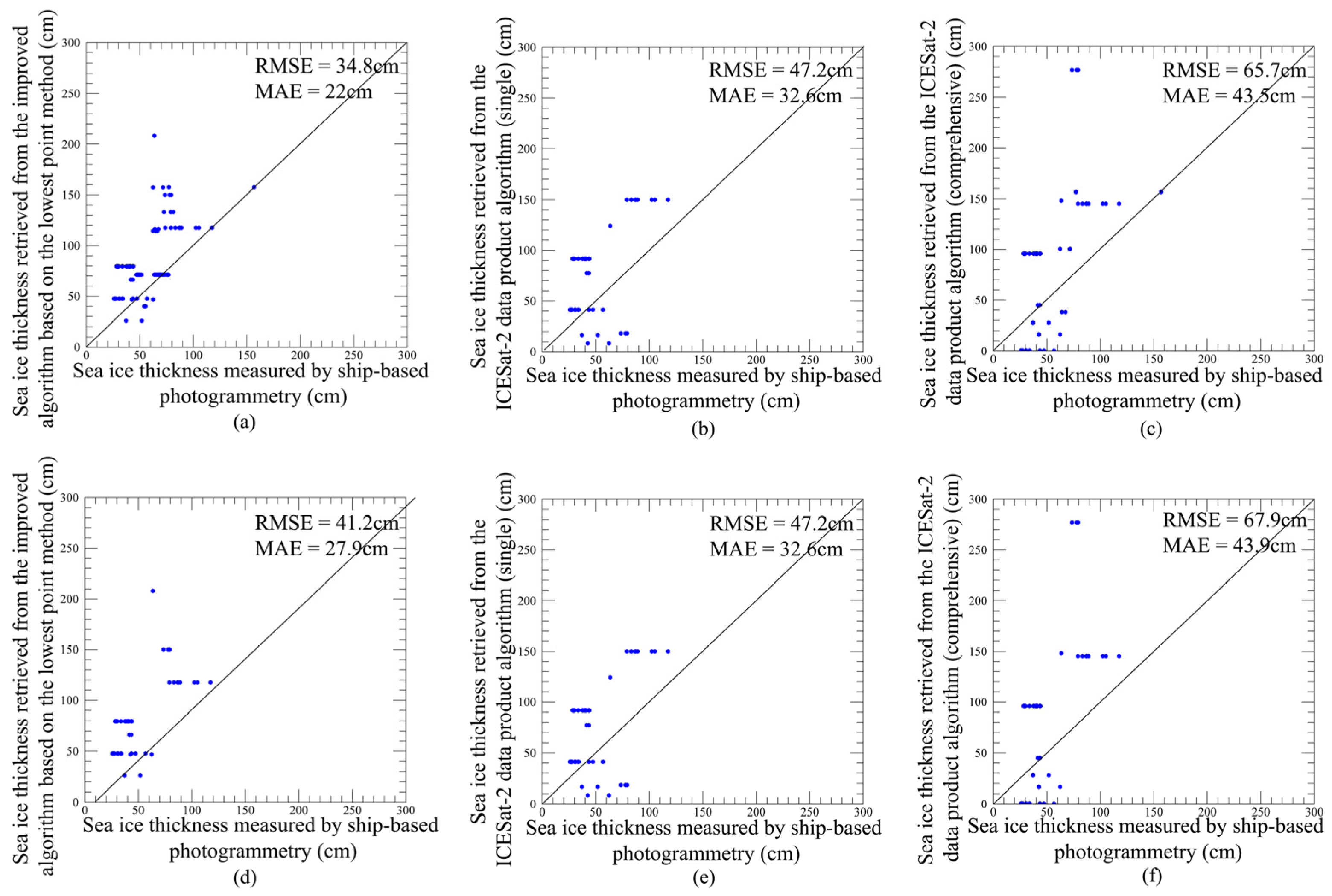
3.4. Accuracy of the Retrieved Antarctic Sea Ice Thickness Based on the Improved Algorithm of the Lowest Point Method

We obtained ship-based observational sea ice thickness data from CHINARE-35 to assess the accuracy of the retrieved Antarctic sea ice thickness, which was calculated from the sea ice freeboard estimated with the improved algorithm of the lowest point method. The Antarctic sea ice thickness calculated from the freeboard estimated with the ICESat-2 data product algorithm was also assessed and compared. The root mean squared error (RMSE) and mean absolute error (MAE) were adopted in this study as assessment indices, which are defined by Equation (4) and Equation (5):
RMSE = j = 1 n ( H i j H p j ) 2 / n
MAE = ( j = 1 n a b s ( H i j H p j ) ) / n
where H i denotes the sea ice thickness retrieved with the improved algorithm of the lowest point method or retrieved with the ICESat-2 data product algorithm, H p is the sea ice thickness measured via ship-based photogrammetry during CHINARE-35, n is the number of comparison pair points, and abs() in Equation (5) means the absolute value function.
Figure 9a–c shows that the RMSE value of the sea ice thickness estimated with the improved algorithm of the lowest point method was 34.8 cm, while the RMSE value of the sea ice thickness estimated with the ICESat-2 data product algorithm (single) and ICESat-2 data product algorithm (comprehensive) was 47.2 cm and 65.7 cm, respectively. Moreover, the MAE values reached 22 cm, 32.6 cm, and 43.5 cm, respectively. Considering that the coverage of these three kinds of data was inconsistent (the coverage of the data estimated with the improved algorithm was slightly higher than that of the other kinds of data), we selected overlapping data and compared the associated RMSE and MAE values. Figure 9d–f shows that the RMSE reached 41.2 cm, 47.2 cm, and 67.9 cm, and the MAE was 27.8 cm, 32.6 cm, and 43.8 cm, respectively. The statistical results are summarized in Table 4. It could be concluded from this that the improved algorithm of the lowest point method used in this study performed better than the ICESat-2 data product algorithm.

4. Discussion

4.1. Improvement in the Variable Lead Proportion for the Retrieval of the Sea Ice Freeboard and Thickness from ICESat-2 Data

The ICESat-2 is a new-generation laser satellite altimeter that provides more accurate surface elevation measurements and additional surface type classifications, including sea ice leads, which could be used for the estimation of the sea ice freeboard [37]. The accuracy of the retrieved freeboard greatly depends on the precision of lead discrimination along ICESat-2 tracks. In this study, we found that there remained errors in the lead discrimination results obtained with the current ICESat-2 data product. The lowest point method is one of the more commonly applied methods for the retrieval of the sea ice freeboard [23], and an important step of this approach is the determination of the lowest point proportion for the retrieval of the Antarctic sea ice freeboard because the distribution of leads varies over time and space in the Antarctic Ocean.
In this study, we proposed an improved algorithm of the lowest point method to calculate the Antarctic sea ice freeboard and thickness from ICESat-2 altimeter data. The proportions of the lowest points (leads) over all 12 months of the year in the different sea areas of the Antarctic Ocean were confirmed according to the combined analysis of ICESat-2 tracks and collocated Sentinel-1 SAR images. Compared to the previous algorithm of the lowest point method [13], the improved algorithm replaced the traditional fixed lead proportion with a variable proportion in each month in the different Antarctic sea areas. The validation results verified that the Antarctic sea ice thickness calculated with the improved algorithm of the lowest point method performed better than that calculated with the ICESat-2 data product algorithm. Although we proposed a variable representative lead proportion for freeboard and sea ice thickness estimation, limitations remain. Since the SAR images obtained in our study could be inaccurate for distinguishing thin sea ice from seawater, our algorithm may overestimate the lead proportions in the lowest point method, resulting in overestimated sea surface height values and underestimated sea ice freeboard and thickness values according to Equation (1) [33]. It indicates that our algorithm has room for improvement, especially in the selection of images, although our algorithm could provide more accurate data than the ICESat-2 data product algorithm.
We also compared the retrieved sea ice thickness based on our algorithm with the results from Xu [38] (https://figshare.com/articles/dataset/Antarctic_Sea-Ice_Thickness_and_Volume_from_NASA_s_ICESat_ICESat-2_Missions/12910121/, accessed on 7 February 2022). As shown in Figure 10, the bias between these two results ranged from −17 cm to 26 cm. The difference between these two results was small in January 2019 and May 2019 with the average value of 2.8 cm.

4.2. Influence of Negative Freeboard for the Retrieval from ICESat-2 Altimeter Data

In the process of sea ice thickness retrieval, we found that there existed negative freeboard in Antarctic Ocean during the study period. As shown in Figure 11a, the negative freeboard occurred mainly in the coastal area of the Weddell Sea and Bellingshausen and Amundsen Sea ranging from −5 cm to 0 cm. Previous studies have shown that snow cover on Antarctic sea ice plays an important role in the formation of negative freeboard because sea ice can be depressed below sea-water level and turned into snow-ice due to the snow loading [39]. It could therefore be seen that negative freeboard was concentrated in the region with great snow depth, especially in the area where there existed multi-year sea ice.
Figure 11b shows the difference between the retrieved sea ice thickness, which did not consider the influence of the negative freeboard and that considering the negative freeboard. It could be perceived that sea ice thickness not considering negative freeboard is 1.86 cm thicker than that considering negative freeboard. The method of dealing with the negative freeboard for the accurate retrieval of Antarctic sea ice thickness will be the focus of our future work.

4.3. Uncertainty in the Sea Ice Freeboard and Thickness Retrieved from ICESat-2 Altimeter Data

There are uncertainties when converting ICESat-2-measured point data into freeboard gridded data with a specific spatial resolution (12.5 km in this study) because of the data processing normally required [15]. We calculated the standard deviation for each freeboard grid in the different months with the improved algorithm of the lowest point method (Figure 12). The mean value of the standard deviation across all sea ice freeboard grids ranged from 9 cm to 17 cm, and the mode of the standard deviation ranged from 1 cm to 8 cm. The mean standard deviation of the sea ice freeboard determined by the ICESat [40] was slightly larger than our result. The high mean standard deviation of the ICESat-2-derived sea ice freeboard was attributed to the smaller footprint of the ICESat-2 than that of the ICESat, which made it easier for the ICESat-2 to capture texture features and detect elevation changes in the sea ice surface. Therefore, the ICESat-2 attained a high standard deviation due to the high accuracy in the rasterization process of freeboard grids with a specific resolution.
In addition, the validity of the coverage of the ICESat-2 laser altimeter data should be further examined because monthly altimeter tracks cannot completely cover the whole Antarctic Ocean [2]. The extent of ICESat-2 operational measurements is concentrated near satellite tracks. We employed AMSR2-unified L3 daily 12.5 km sea ice concentration data to verify the representativeness of ICESat-2 altimeter data. The total number of grids with AMSR2-derived sea ice concentrations higher than 0% at the ICESat-2 measuring data grid scale was counted to calculate the proportion of valid ICESat-2 measurement data in the ice-covered areas of the Antarctic (Figure 13). The proportion of valid ICESat-2 measurement data in the Antarctic sea ice region ranged from 9.5% to 36%. Generally, the proportion was high when the sea ice extent was small because the ICESat-2 tracks were more intensive in the coastal areas. The average proportion of sea ice-covered 12.5-km grids with valid ICESat-2 data that could be considered for sea ice thickness retrieval in the Weddell Sea, Indian Ocean, Pacific Ocean, Ross Sea, Bellingshausen and Amundsen Sea was 24.5%, 17.4%, 14.0%, 28.1%, and 18.7%, respectively. The difference between the maximum and minimum proportions in the different Antarctic sea areas was 14.1%, which indicates that ICESat-2 altimeter data exhibit different representativeness levels among the various sea areas. Therefore, the Antarctic sea ice thickness retrieved from the ICESat-2 altimeter data could be considered more typical in the Weddell Sea and Ross Sea and less typical in the Indian Ocean and Pacific Ocean. The ICESat-2 improved the accuracy and the amount of satellite measurement data along its tracks. However, the altimeter data coverage in the Antarctic Ocean is not higher than that of the previous generation of altimeter satellites.
According to Equation (3), the sea ice density, snow density, and seawater density contribute to the retrieval of the Antarctic sea ice thickness from the ICESat-2 altimeter data. The seawater density contributes the least to the uncertainty in the estimation of the sea ice thickness, while the sea ice density contributes the most to the uncertainty [41]. We obtained the uncertainty in the sea ice density, snow density, and seawater density from the literature [42,43], which reported that the uncertainty in the seawater density, snow density, and sea ice density reached 0.5 kg/m3, 50 kg/m3, and 15 kg/m3, respectively. Calculated with the error propagation model, the influence of the sea ice density, snow density, and seawater density on the retrieval of the sea ice thickness reached 0.19 m, 0.07 m, and 0.01 m, respectively. The sea ice density exerted a great impact on the accuracy of sea ice thickness retrieval from ICESat-2 data, followed by the snow density and seawater density.

4.4. Limitation of the Calculated Lead Proportions along ICESat-2 Measurement Points Based on Sentinel-1 SAR Images

Sentinel-1 SAR images were used in this study and collocated with ICESat-2 tracks to calculate the variable lead proportions along ICESat-2 measurement points for the retrieval of the Antarctic sea ice freeboard and thickness. The uncertainty in these derived lead proportions entails the fact that not all ICESat-2 tracks were involved in the proportion calculation, as limited by the number of matched SAR images. Compared to SAR images, optical images are often affected by clouds. However, optical remote sensing can better distinguish thin sea ice from melting ice under cloudless weather conditions [44]. The ability of SAR images to identify thin sea ice and melted ice increases the uncertainty in the calculated lead proportions along the ICESat-2 measurement points.
The mean value of the lead proportion was applied to represent the overall lead distribution along the ICESat-2 tracks within a given month of the year. The uncertainty due to the fluctuation in the lead proportion along the different ICESat-2 tracks is given in Table 3. The standard deviation of the lead proportions in the different months in the various Antarctic sea areas ranged from 0.49% to 4.29%, which could cause a freeboard uncertainty ranging from 0.03 m to 0.05 m and a sea ice thickness uncertainty ranging from 0.28 m to 0.43 m. In theory, each ICESat-2 track yields a corresponding lead proportion for determining the local sea surface height for the retrieval of the Antarctic sea ice freeboard and thickness. However, this scheme could not be adopted because of the lack of enough matched images in the practical calculation process. Therefore, combining multiple types of remote sensing images (both SAR and optical images) to obtain more accurate Antarctic lead proportions along ICESat-2 tracks will comprise our future work.

5. Conclusions

The ICESat-2 is a new-generation altimeter that provides high-resolution surface height measurements for the retrieval of the Antarctic sea ice freeboard and thickness. Our present study first assessed the accuracy of lead discrimination from the currently released ICESat-2 data product based on Sentinel-1 SAR images and then explored an improved algorithm involving variable lead proportions based on the lowest point method for the retrieval of the Antarctic sea ice freeboard and sea ice thickness from November 2018 to October 2019. The retrieved Antarctic sea ice thickness was finally compared to ship-based observational sea ice thickness values during CHINARE-35.
There occurred a large number of ICESat-2 measurement points in the data product that were misclassified according to the obtained Sentinel-1 SAR images. The accuracy of lead classification with the ICESat-2 data product algorithm reached only up to 40% of that of Sentinel-1-extracted sea ice lead classification, which could cause substantial errors in the retrieval of the sea ice freeboard and thickness from the ICESat-2 altimeter data. The Antarctic sea ice freeboard calculated with the improved algorithm of the lowest point method was 0.5 cm to 2.2 cm larger than that calculated with the ICESat-2 data product algorithm. The improved algorithm of the lowest point method for sea ice thickness retrieval performed better than did the ICESat-2 data product algorithm when validated against ship-based observational sea ice thickness data. The sea ice thickness in the Antarctic Ocean exhibited the characteristics of thicker ice concentrated along the coast and thinner ice distributed offshore, with thicker ice in the Antarctic winter and thinner ice in summer. The thickest sea ice was distributed in the West Weddell Sea near the Antarctic Peninsula.
The uncertainties in the sea ice density, snow density, and seawater density in the retrieval of the sea ice thickness were 0.19 m, 0.07 m, and 0.01 m, respectively. In addition, applying a representative lead proportion in the different months in the various Antarctic sea areas could cause a sea ice thickness uncertainty ranging from 0.28 m to 0.43 m. Because the insufficient ability of SAR images to identify thin sea ice and melted ice increased the uncertainty in the calculated lead proportions along the ICESat-2 measurement points, combining multiple types of remote sensing images (SAR and optical images) in the Antarctic to obtain more accurate Antarctic lead proportions along ICESat-2 tracks comprises our further work.

Author Contributions

Conceptualization, X.P. and Q.J.; methodology, X.P. and Y.C.; validation, G.L. and L.S.; formal analysis, Q.J.; investigation, Y.C. and Z.L.; resources, X.P. and Q.J.; data curation, Q.J.; writing—original draft preparation, X.P. and Y.C.; writing—review and editing, X.P. and Y.C.; supervision, X.P.; project administration, L.S. and M.L.; funding acquisition, X.P. and Y.C. All authors have read and agreed to the published version of the manuscript.

Funding

This work was supported by the National Natural Science Foundation of China under Grant No. 42076235, the National Key Research and Development Program of China under Grant No. 2017FYA0603104, the Special Fund for High Resolution Images Surveying and Map-ping Application System under Grant No.42-Y30B04-9001-19/21, and the Spatial Fund of Chinese Arctic and Antarctic Administration under Grant No. IRASCC2020-2022-No.01-01-03.

Data Availability Statement

The data is available to readers by contacting the corresponding author.

Acknowledgments

The authors thank the members of the 35th Chinese National Antarctic Re-search Expedition and the crews of R/V Xuelong for their assistance during the ship-based sea ice thickness observations.

Conflicts of Interest

The authors declare that they have no known competing financial interests or personal relationships that could have appeared to influence the work reported in this paper.

References

  1. Turner, J.; Comiso, J.C.; Marshall, G.J.; Lachlan-Cope, T.A.; Bracegirdle, T.; Maksym, T.; Meredith, M.P.; Wang, Z.; Orr, A. Non-annular atmospheric circulation change induced by stratospheric ozone depletion and its role in the recent increase of Antarctic sea ice extent. Geophys. Res. Lett. 2009, 36, L08502. [Google Scholar] [CrossRef] [Green Version]
  2. Li, H.; Xie, H.; Kern, S.; Wan, W.; Ozsoy, B.; Ackley, S.; Hong, Y. Spatio-temporal variability of Antarctic sea-ice thickness and volume obtained from ICESat data using an innovative algorithm. Remote Sens. Environ. 2018, 219, 44–61. [Google Scholar] [CrossRef]
  3. Comiso, J.C.; Parkinson, C.; Gersten, R.; Stock, L. Accelerated decline in the Arctic sea ice cover. Geophys. Res. Lett. 2008, 35. [Google Scholar] [CrossRef] [Green Version]
  4. Tian, L.; Xie, H.; Ackley, S.F.; Tang, J.; Mestas-Nuñez, A.M.; Wang, X. Sea-ice freeboard and thickness in the Ross Sea from airborne (IceBridge 2013) and satellite (ICESat 2003–2008) observations. Ann. Glaciol. 2020, 61, 24–39. [Google Scholar] [CrossRef] [Green Version]
  5. Kwok, R. Satellite remote sensing of sea-ice thickness and kinematics: A review. J. Glaciol. 2010, 56, 1129–1140. [Google Scholar] [CrossRef] [Green Version]
  6. Kurtz, N.T.; Galin, N.; Studinger, M. An improved CryoSat-2 sea ice freeboard retrieval algorithm through the use of waveform fitting. Cryosphere 2014, 8, 1217–1237. [Google Scholar] [CrossRef] [Green Version]
  7. Kwok, R.; Zwally, H.J.; Yi, D. ICESat observations of Arctic sea ice: A first look. Geophys. Res. Lett. 2004, 31, L16401. [Google Scholar] [CrossRef] [Green Version]
  8. Laxon, S.W.; Giles, K.A.; Ridout, A.L.; Wingham, D.J.; Willatt, R.; Cullen, R.; Kwok, R.; Schweiger, A.; Zhang, J.; Hass, C.; et al. CryoSat-2 estimates of Antarctic sea ice thickness and volume. Geophys. Res. Lett. 2013, 40, 732–737. [Google Scholar] [CrossRef] [Green Version]
  9. Xie, H.; Ackley, S.; Yi, D.; Zwally, H.; Wagner, P.; Weissling, B.; Lewis, M.; Ye, K. Sea-ice thickness distribution of the Bellingshausen Sea from surface measurements and ICESat altimetry. Deep Sea Res. Part II Top. Stud. Oceanogr. 2011, 58, 1039–1051. [Google Scholar] [CrossRef]
  10. Xie, H.; Tekeli, A.E.; Ackley, S.F.; Yi, D.; Zwally, H.J. Sea ice thickness estimations from ICESat Altimetry over the Bellingshausen and Amundsen Seas, 2003–2009. J. Geophys. Res. Oceans 2013, 118, 2438–2453. [Google Scholar] [CrossRef]
  11. Holland, M.M.; Bitz, C.; Hunke, E.C.; Lipscomb, W.H.; Schramm, J.L. Influence of the Sea Ice Thickness Distribution on Polar Climate in CCSM3. J. Clim. 2006, 19, 2398–2414. [Google Scholar] [CrossRef] [Green Version]
  12. Yang, Q.; Losa, S.N.; Losch, M.; Tian-Kunze, X.; Nerger, L.; Liu, J.; Kaleschke, L.; Zhang, Z. Assimilating SMOS sea ice thickness into a coupled ice-ocean model using a local SEIK filter. J. Geophys. Res. Oceans 2014, 119, 6680–6692. [Google Scholar] [CrossRef] [Green Version]
  13. Zwally, H.J.; Yi, D.; Kwok, R.; Zhao, Y. ICESat measurements of sea ice freeboard and estimates of sea ice thickness in the Weddell Sea. J. Geophys. Res. Ocean. 2008, 113. [Google Scholar] [CrossRef] [Green Version]
  14. Yi, D.; Zwally, H.J.; Robbins, J.W. ICESat observations of seasonal and interannual variations of sea-ice freeboard and estimated thickness in the Weddell Sea, Antarctica (2003–2009). Ann. Glaciol. 2011, 52, 43–51. [Google Scholar] [CrossRef] [Green Version]
  15. Kern, S.; Ozsoy-Çiçek, B.; Worby, A.P. Antarctic Sea-Ice Thickness Retrieval from ICESat: Inter-Comparison of Different Approaches. Remote Sens. 2016, 8, 538. [Google Scholar] [CrossRef] [Green Version]
  16. Lee, S.; Im, J.; Kim, J.; Kim, M.; Shin, M.; Kim, H.-C.; Quackenbush, L.J. Arctic Sea Ice Thickness Estimation from CryoSat-2 Satellite Data Using Machine Learning-Based Lead Detection. Remote Sens. 2016, 8, 698. [Google Scholar] [CrossRef] [Green Version]
  17. Kwok, R.; Kacimi, S. Three years of sea ice freeboard, snow depth, and ice thickness of the Weddell Sea from Operation IceBridge and CryoSat-2. Cryosphere 2018, 12, 2789–2801. [Google Scholar] [CrossRef] [Green Version]
  18. Landy, J.C.; Petty, A.A.; Tsamados, M.; Stroeve, J.C. Sea Ice Roughness Overlooked as a Key Source of Uncertainty in CryoSat-2 Ice Freeboard Retrievals. J. Geophys. Res. Ocean. 2020, 125, e2019JC015820. [Google Scholar] [CrossRef]
  19. Kern, S.; Spreen, G. Uncertainties in Antarctic sea-ice thickness retrieval from ICESat. Ann. Glaciol. 2017, 56, 107–119. [Google Scholar] [CrossRef] [Green Version]
  20. Markus, T.; Neumann, T.; Martino, A.; Abdalati, W.; Brunt, K.; Csatho, B.; Farrell, S.; Fricker, H.; Gardner, A.; Harding, D.; et al. The Ice, Cloud, and land Elevation Satellite-2 (ICESat-2): Science requirements, concept, and implementation. Remote Sens. Environ. 2017, 190, 260–273. [Google Scholar] [CrossRef]
  21. Kwok, R.; Cunningham, G.; Markus, T.; Hancock, D.; Morison, J.H.; Palm, S.P.; Farrell, S.L.; Ivanoff, A.; Wimert, J.; The ICESat-2 Science Team. ATLAS/ICESat-2 L3A Sea Ice Freeboard, Version 3; NSIDC—National Snow and Ice Data Center: Boulder, CO, USA, 2020. [Google Scholar]
  22. Kwok, R.; Kacimi, S.; Markus, T.; Kurtz, N.T.; Studinger, M.; Sonntag, J.G.; Manizade, S.S.; Boisvert, L.N.; Harbeck, J.P. ICESat-2 Surface Height and Sea Ice Freeboard Assessed with ATM Lidar Acquisitions from Operation IceBridge. Geophys. Res. Lett. 2019, 46, 11228–11236. [Google Scholar] [CrossRef]
  23. Wang, X.; Xie, H.; Ke, Y.; Ackley, S.F.; Liu, L. A method to automatically determine sea level for referencing snow freeboards and computing sea ice thicknesses from NASA IceBridge airborne LIDAR. Remote Sens. Environ. 2013, 131, 160–172. [Google Scholar] [CrossRef]
  24. Shokr, M.; Sinha, N. Sea Ice: Physics and Remote Sensing, 1st ed.; Shokr, M.E., Sinha, N., Eds.; American Geophysical Union: Washington, DC, USA, 2015. [Google Scholar]
  25. Weissling, B.; Lewis, M.; Ackley, S. Sea-ice thickness and mass at Ice Station Belgica, Bellingshausen Sea, Antarctica. Deep Sea Res. Part II Top. Stud. Oceanogr. 2011, 58, 1112–1124. [Google Scholar] [CrossRef]
  26. Simmondsxs, I.; Budd, W.F. Sensitivity of the southern hemisphere circulation to leads in the Antarctic pack ice. Q. J. R. Meteorol. Soc. 1991, 117, 1003–1024. [Google Scholar] [CrossRef]
  27. Beitsch, A.; Kaleschke, L.; Kern, S. Investigating High-Resolution AMSR2 Sea Ice Concentrations during the February 2013 Fracture Event in the Beaufort Sea. Remote Sens. 2014, 6, 3841–3856. [Google Scholar] [CrossRef] [Green Version]
  28. Lee, Y.-K.; Kongoli, C.; Key, J. An In-Depth Evaluation of Heritage Algorithms for Snow Cover and Snow Depth Using AMSR-E and AMSR2 Measurements. J. Atmos. Ocean. Technol. 2015, 32, 2319–2336. [Google Scholar] [CrossRef]
  29. Markus, T.; Cavalieri, D.J. Snow Depth Distribution over Sea Ice in the Southern Ocean from Satellite Passive Micro-Wave Data; American Geophysical Union: Washington, DC, USA, 1998. [Google Scholar]
  30. Shi, L.; Karvonen, J.; Cheng, B.; Vihma, T.; Lin, M.; Liu, Y.; Wang, Q.; Jia, Y. Sea ice thickness retrieval from SAR imagery over Bohai sea. In Proceedings of the 2014 IEEE Geoscience and Remote Sensing Symposium, Quebec City, QC, Canada, 13–18 July 2014; pp. 4864–4867. [Google Scholar] [CrossRef]
  31. Mei, H.; Lu, P.; Wang, Q.; Cao, X.; Li, Z. Study of the spatiotemporal variations of summer sea ice thickness in the Pacific arctic sector based on shipside images. Chin. J. Polar Res. 2021, 2021, 37–48. (In Chinese) [Google Scholar]
  32. Kwok, R.; Kacimi, S.; Webster, M.; Kurtz, N.; Petty, A. Arctic Snow Depth and Sea Ice Thickness From ICESat-2 and CryoSat-2 Freeboards: A First Examination. J. Geophys. Res. Ocean. 2020, 125, e2019JC016008. [Google Scholar] [CrossRef]
  33. Kwok, R.; Petty, A.A.; Bagnardi, M.; Kurtz, N.T.; Cunningham, G.F.; Ivanoff, A.; Kacimi, S. Refining the sea surface identification approach for determining freeboards in the ICESat-2 sea ice products. Cryosphere 2021, 15, 821–833. [Google Scholar] [CrossRef]
  34. Kurtz, N.T.; Markus, T. Satellite observations of Antarctic sea ice thickness and volume. J. Geophys. Res. 2012, 117, C08025. [Google Scholar] [CrossRef] [Green Version]
  35. Parkinson, C.L.; Cavalieri, D.J. Antarctic Sea Ice Variability and Trends, 1979–2010. Cryosphere 2012, 6, 871–880. [Google Scholar] [CrossRef] [Green Version]
  36. Lange, M.A.; Eicken, H. The sea ice thickness distribution in the northwestern Weddell Sea. J. Geophys. Res. Ocean. 1991, 96, 4821–4837. [Google Scholar] [CrossRef]
  37. Neumann, T.A.; Martino, A.J.; Markus, T.; Bae, S.; Bock, M.R.; Brenner, A.C.; Brunt, K.M.; Cavanaugh, J.; Fernandes, S.T.; Hancock, D.W.; et al. The Ice, Cloud, and Land Elevation Satellite-2 mission: A global geolocated photon product derived from the Advanced Topographic Laser Altimeter System. Remote Sens. Environ. 2019, 233, 111325. [Google Scholar] [CrossRef] [PubMed]
  38. Xu, Y.; Li, H.; Liu, B.; Xie, H.; Ozsoy-Cicek, B. Deriving Antarctic Sea-Ice Thickness from Satellite Altimetry and Estimating Consistency for NASA’s ICESat/ICESat-2 Missions. Geophys. Res. Lett. 2021, 48, e2021GL093425. [Google Scholar] [CrossRef]
  39. Eicken, H.; Fischer, H.; Lemke, P. Effects of the snow cover on Antarctic sea ice and potential modulation of its response to climate change. Ann. Glaciol. 1995, 21, 369–376. [Google Scholar] [CrossRef] [Green Version]
  40. Kwok, R.; Cunningham, G.F.; Zwally, H.J.; Yi, D. Ice, Cloud, and land Elevation Satellite (ICESat) over Arctic sea ice: Retrieval of freeboard. J. Geophys. Res. Ocean. 2007, 112, C12013. [Google Scholar] [CrossRef] [Green Version]
  41. Spreen, G.; Kern, S.; Stammer, D.; Forsberg, R.; Haarpaintner, J. Satellite-based estimates of sea-ice volume flux through Fram Strait. Ann. Glaciol. 2006, 44, 321–328. [Google Scholar] [CrossRef] [Green Version]
  42. Massom, R.A.; Eicken, H.; Haas, C.; Jeffries, M.O.; Drinkwater, M.R.; Sturm, M.; Worby, A.P.; Wu, X.; Lytle, V.I.; Ushio, S.; et al. Snow on Antarctic sea ice. Rev. Geophys. 2001, 39, 413–445. [Google Scholar] [CrossRef] [Green Version]
  43. Maksym, T.; Markus, T. Antarctic sea ice thickness and snow-to-ice conversion from atmospheric reanalysis and passive microwave snow depth. J. Geophys. Res. 2008, 113, C02S12. [Google Scholar] [CrossRef]
  44. Li, W.; Liu, L.; Zhang, J. Fusion of SAR and Optical Image for Sea Ice Extraction. J. Ocean Univ. China 2021, 20, 1440–1450. [Google Scholar] [CrossRef]
Figure 1. Five sea areas of the Antarctic Ocean, with overlaid background of the maximum (blue, 20 September 2019) and minimum (light green, 20 January 2019) Antarctic sea ice extents from November 2018 to October 2019. The whole Antarctic Ocean refers to the sea areas around the Antarctic continent, which is higher than 60°S.
Remotesensing 14 01069 g001
Figure 2. Ship routes during CHINARE-35 with (a) the ship-based observational sea ice thickness (red dots) and (b) sea ice thickness estimation software involving photogrammetric images. The red lines in (b) mean the length of reference ball and sea ice thickness and the blue line means snow depth. The red area at the bottom of (b) is the side of this ship.
Remotesensing 14 01069 g002
Figure 3. Example of an ICESat-2 track crossing (a) an original Sentinel-1 SAR image and (b) discriminated leads from the same Sentinel-1 image. The red line in (b) indicates the part of the ICESat-2 track that is classified as a lead based on the Sentinel image-1. The lead proportion along this ICESat-2 track can be calculated by the ratio of the red line length to the ICESat-2 track length in the Sentinel-1 image.
Remotesensing 14 01069 g003
Figure 4. Geometric relationships between total freeboard ( H f ), snow depth ( H f s ), and sea ice thickness ( H i ) measured by ICESat-2 satellite altimeter. Sea ice freeboard in this study refers to total freeboard ( H f ).
Remotesensing 14 01069 g004
Figure 5. Sea ice and leads in Sentinel-1 SAR and Sentinel-2 optical images at different times within a day: (a) Sentinel-1 image at 3:06, 17 November 2018, (b) Sentinel-1 image at 3:56, 17 November 2018, (c) Sentinel-1 image at 7:13, 17 November 2018, and (d) Sentinel-2 image at 19:04, 17 November 2018.
Remotesensing 14 01069 g005
Figure 6. Comparison of the surface type classification results between the ICESat-2 data product algorithm and Sentinel-1 SAR images: (a) ICESat-2 ATL-07 data at 8:25, 8 October 2019, with the background of a Sentinel-1 image at 7:55, 8 October 2019, (b) ICESat-2 ATL-07 data at 6:01, 18 June 2019, with the background of a Sentinel-1 image at 7:27, 18 June 2019, (c) the distribution of leads in the ICESat-2 labeled surface type (red) and Sentinel-1 image (blue) along one beam with most leads along the ICESat-2 tracks in (a), and (d) the distribution of leads in the ICESat-2 labeled surface type (red) and Sentinel-1 image (blue) along one beam with most leads along the ICESat-2 tracks in (b).
Remotesensing 14 01069 g006
Figure 7. Mean sea ice freeboard calculated with the improved algorithm of the lowest point method and ICESat-2 data product algorithm in the Antarctic Ocean: (a) the whole Antarctic Ocean, (b) the Weddell Sea, (c) the Indian Ocean, (d) the Pacific Ocean, (e) the Ross Sea, and (f) the Bellingshausen and Amundsen Sea.
Remotesensing 14 01069 g007
Figure 8. Antarctic sea ice thickness calculated with the improved algorithm of the lowest point method and ICESat-2 measured surface height data from November 2018 to October 2019.
Remotesensing 14 01069 g008
Figure 9. Comparison of the sea ice thickness values estimated with the ICESat-2 data product algorithm and the improved algorithm of the lowest point methods to the sea ice thickness measured via ship-based photogrammetry during CHINARE-35: (a) assessment of the sea ice thickness retrieved with the improved algorithm of the lowest point method, (b) assessment of the sea ice thickness retrieved with the ICESat-2 data product algorithm (single), (c) assessment of the sea ice thickness retrieved with the ICESat-2 data product algorithm (comprehensive), (d) assessment of the sea ice thickness retrieved with the improved algorithm of the lowest point method in overlapping data, (e) assessment of the sea ice thickness retrieved with the ICESat-2 data product algorithm (single) in overlapping data, and (f) assessment of the sea ice thickness retrieved with the ICESat-2 data product algorithm (comprehensive) in overlapping data.
Remotesensing 14 01069 g009
Figure 10. Monthly difference between sea ice thickness obtained from our improved algorithm and Xu [38] from November 2018 to October 2019.
Remotesensing 14 01069 g010
Figure 11. The contribution of negative freeboard in the retrieval of sea ice freeboard and thickness from ICESat-2 altimeter data using out algorithm from November 2018 to October 2019 (a) and the difference between sea ice thickness that did not consider negative freeboard and sea ice thickness considering negative freeboard from November 2018 to October 2019 (b).
Remotesensing 14 01069 g011
Figure 12. Frequency histogram of the standard deviation of the sea ice freeboard calculated with the improved algorithm of the lowest point method from November 2018 to October 2019.
Remotesensing 14 01069 g012
Figure 13. Proportion of valid ICESat-2 measurement data in the ice-covered areas of the Antarctic from November 2018 to October 2019. The ice-covered areas were confirmed against AMSR2 12.5-km sea ice concentration data: (a) proportion in the whole Antarctic Ocean, (b) proportion in the Weddell Sea, (c) proportion in the Indian Ocean, (d) proportion in the Pacific Ocean, (e) proportion in the Ross Sea, and (f) proportion in the Bellingshausen and Amundsen Sea.
Remotesensing 14 01069 g013
Table 1. Information on the satellite images used in this study.
Satellite DesignationImage TypeResolutionNumber of Images Used in This Study
Sentinel-1A, Sentinel-1BSAR image40 m213
Sentinel-2A, Sentinel-2BOptical image10 m10
Table 2. Accuracy of the labeled surface type from ICESat-2 ATL-07 data (6 beams) assessed against collocated Sentinel-1 images.
DateTrackICESat-2
CLASSIFIED AS A LEADCorrect ClassificationIncorrect ClassificationMissing Lead DiscriminationNumber of Leads in Sentinel-1Accuracy of
ICESat-2 Lead Discrimination (%)
8 October 20191008-gt1l395143812122263.54
1008-gt1r468184501611793.85
1008-gt2l77532944663496342.45
1008-gt2r81511769871282914.36
1008-gt3l9449884620730510.38
1008-gt3r116721295525046218.17
18 June 20190618-gt1l7727566682.60
0618-gt1r6936639424.35
0618-gt2l56947526116.07
0618-gt2r44836758318.18
0618-gt3l7217559411123.61
0618-gt3r380381161160
Table 3. Proportions of leads along the ICESat-2 tracks in the Antarctic Ocean from November 2018 to October 2019 calculated from Sentinel-1 SAR images.
Year/MonthLead Proportion along ICESat-2 Tracks (%)
Weddell SeaRoss SeaBellingshausen and Amundsen SeaIndian OceanPacific Ocean
2018/112.606.672.983.932.96
2018/126.114.593.712.695.69
2019/013.445.822.711.532.80
2019/022.933.996.422.843.04
2019/031.183.172.131.692.97
2019/041.941.102.272.142.78
2019/051.551.992.511.961.62
2019/061.811.983.071.502.44
2019/071.600.731.971.172.47
2019/082.473.082.670.822.78
2019/091.922.531.081.692.74
2019/104.234.271.733.463.52
Mean value2.653.332.772.122.99
Table 4. Comparison of the sea ice thickness values retrieved based on the ICESat-2 data product algorithm and the improved algorithm in this study to the ship-based measured sea ice thickness during CHINARE-35.
Algorithms for the Retrieval of the Sea Ice Thickness from ICESat-2 dataRMSE (cm)MAE (cm)
Improved algorithm of the lowest point method34.822.0
ICESat-2 data product algorithm (single)47.232.6
ICESat-2 data product algorithm (comprehensive)65.743.5
Improved algorithm of the lowest point method in overlapping data41.227.9
ICESat-2 data product algorithm (single) in overlapping data47.232.6
ICESat-2 data product algorithm (comprehensive) in overlapping data67.943.9
Publisher’s Note: MDPI stays neutral with regard to jurisdictional claims in published maps and institutional affiliations.

