
Remote Sensing to Characterize River Floodplain Structure and Function

1
Flathead Lake Biological Station, University of Montana, Polson, MT 59864, USA
2
Freshwater Map, P.O. Box 166, Bigfork, MT 59911, USA
3
Center for Ecology, Evolution and Biogeochemistry (CEEB), Department of Aquatic Ecology, EAWAG, 6047 Kastanienbaum, Switzerland
*
Author to whom correspondence should be addressed.
Remote Sens. 2022, 14(5), 1132; https://0-doi-org.brum.beds.ac.uk/10.3390/rs14051132
Submission received: 25 December 2021
/
Revised: 16 February 2022
/
Accepted: 23 February 2022
/
Published: 25 February 2022
(This article belongs to the Special Issue Remote Sensing of Fluvial Systems)
Abstract
:Advancing understanding of the complexities and expansive spatial scales of river ecology can be enhanced through the application of remote sensing. We obtained satellite (Quickbird) and airborne (LIDAR, hyperspectral, multispectral, and thermal) imagery data of an alluvial gravel-bed river floodplain in western Montana to quantify both riparian and aquatic habitats and processes. LIDAR data provided a detailed bare earth DEM and vegetation canopy DEM. We classified river hydraulics and aquatic habitats using a combination of the satellite multispectral, airborne hyperspectral, and LIDAR data coupled with spatially-explicit acoustic Doppler velocity profile data of water depth and velocity. Velocity, depth, and Froude classifications were aggregated into similar hydraulic zones of river habitat classes. Thermal imagery data were coupled with field measurements of temperature and radon gas tracer to identify patterns of water exchange between the alluvial aquifer and the surface. We found a high complexity of aquatic surface temperatures and radon tracer linked to groundwater discharge from the alluvial aquifer. Airborne hyperspectral data were used to identify “hot spots” of periphyton production, which coincided with the complex nature of groundwater–surface water exchange. Airborne hyperspectral data provided differentiation of vegetation patches by dominant species. When the hyperspectral data were coupled to LIDAR first return metrics, we were able to determine vegetation canopy height and relative vegetation patch age classes. The integration of these various remote sensing sources allowed us to characterize the distribution and abundance of floodplain aquatic and riparian species and model processes of change through space and time.
1. Introduction
River floodplains provide a critical habitat for a wide array of aquatic, terrestrial, and avian species [1,2,3]. Unfortunately, because of the pervasiveness of dams, levees, transportation corridors, and other factors that encroach on river hydrologic regimes and/or geomorphic processes, they are also among the most endangered landscapes on the planet [4,5]. Natural, unaltered floodplains are composed of multiple, dynamic habitat mosaics [6] that change spatially due to physical drivers, particularly flooding and sediment transport [7,8]. This complex, ever-changing biophysical system, characterized as a shifting habitat mosaic [7], is a fundamental ecosystem attribute affecting the structures and processes of floodplains. While this is true for virtually all river–floodplain systems worldwide, the shifting habitat mosaic is exceptionally dynamic and bio-complex among alluvial gravel-bed rivers.
The legacy of floodplain cut and fill alluviation also creates a complex floodplain topography and channel bathymetry that affords many different aquatic and riparian habitat types. Flow pathways for surface water infiltrating into the alluvial aquifer create a riverine hyporheic zone [9] that results in surface/subsurface water exchange influencing surface and subsurface habitats throughout the floodplain. The hydrological exchange occurs between river water and groundwater in expansive and geomorphologically heterogeneous gravel-bed river floodplains, which are filled with coarse-grained materials (i.e., cobble, gravel, and sand) that express a high hydraulic conductivity [10]. Knowledge of groundwater flow paths, groundwater residence times, the occurrence of localized up- and downwelling, and where mixing takes place is a prerequisite to understanding the creation and maintenance of both groundwater and surface water habitats in alluvial floodplains and across their surfaces. Diverse aquatic habitats on floodplain surfaces, such as springbrooks, side channels, ponds, oxbows, and backwaters, are maintained by their connectivity to the groundwater. Biologically crucial aquatic floodplain habitats are characterized by the amount and the type of groundwater they receive [11]. Hence, understanding aquatic floodplain habitats and their connectivity to the groundwater is necessary for their bio-physical and chemical characterization.
Likewise, riparian vegetation responds to patterns of hydrologic and geomorphic variation. Vegetation establishment primarily occurs on newly deposited sediments appearing on gravel bars following annual spring flooding. Maturing vegetation, which occurs on paleo-floodplain surfaces [7], provides energy reduction and resistance to erosion and alters flow patterns and sediment erosion/deposition patterns [12]. The result is bio-engineering feedback to floodplain evolution and the creation of habitat complexity that is widely distributed across the surface and embedded within the floodplain bed sediments. Scour, deposition, inundation, and drought (and sometimes fire [13]) control the connection and disconnection of these dynamic biophysical structures and processes [8].
High variation in the maximum annual discharge from year to year leads to extremely active floodplain surfaces. The parafluvial zones of the floodplain [7] (i.e., scoured cobble and gravel bars) are frequently inundated and scoured, resetting the temporal terrestrialization of the floodplain surfaces. The orthofluvial zones of the floodplain [7] (i.e., older, vegetated surfaces) are characterized by flood inundation, but with energy being dissipated by mature vegetation, less scour, and much deposition of fines. Thus, patches of floodplain surface appear across an array of successional stages of terrestrial vegetation. These stages generally culminate in mature floodplain gallery forests; however, this successional vegetation trajectory is often interrupted and reset in time and space as the river floods, scours, and redeposits sediment. Human modifications that truncate or amplify hydrologic or geomorphic processes will have cascading effects on floodplain simplification by shifting the thresholds of complexity and connectivity, as well as ecological resilience or resistance [14].
Quantifying river channel and off-channel surface aquatic and terrestrial habitats, especially within river floodplains, is of great interest among river ecologists, hydrologists, geomorphologists, fisheries biologists, conservation biologists, and regulatory agencies [15,16,17,18,19,20]. Quantifying aquatic and riparian floodplain habitats is particularly difficult when employing traditional survey methods because of the high diversity and frequency of change in river environments. For several decades, different field survey techniques have been used to estimate aquatic spatial distribution and abundance of habitat [21]. However, these field survey techniques, especially in large rivers, are limited by the field effort required and are often fraught with high variance in both qualifying and quantifying habitat [22,23]. This is further complicated by the extremely high variation when examining repeatability between different field teams conducting the surveys. These inherent data collection problems (it may take weeks or months to complete even a few kilometers of river length when attempting high precision and detailed measures) are further complicated by changes in river discharge that affect depth, velocity, hydraulics, inundation, and channel connectivity in relation to field data collection time.
Various methodologies have been developed to model river hydraulics from first principles of flow dynamics. For example, the physical habitat simulation (PHABSIM) model, an incremental method for the determination of habitat at various discharge levels, is based on a one-dimensional hydraulics model and has been used extensively to provide a prediction of physical habitat for fish and other species [24,25,26]. However, PHABSIM models generally lack verifiable predictions between the physical habitat and measures of organismal response, such as fish spawning or density [27,28]. Complex flow hydraulics, typical of streams and rivers, pose a significant modeling challenge when trying to quantify spatial complexity and range of channel habitat. This is especially true when trying to assess change in hydraulics and habitat as a function of discharge variability. Studies of the limitations in the transect-based, one-dimensional hydraulic modeling in PHABSIM began incorporating two-dimensional models that better define depth and velocity in the modeled river channel [29,30,31]. Nonetheless, the accuracy of these models, as a function of channel geometry and instream flow measures, remains elusive and only represents a small fraction of the total river.
Kondolf et al. [32] reviewed the assumptions, accuracy, and precision of both one-dimensional and two-dimensional hydraulic modeling and the measurements that provide input data for these models. They concluded that highly accurate hydraulic modeling “seems infeasible for streams with complex channel geometry.” However, as we illustrate in this paper, river mapping approaches employing rapid hydro-acoustic data coupled with survey-grade GPS data and remotely sensed imagery allow river mapping over tens and hundreds of kilometers of rivers geospatially, providing channel and flow complexity as well as the ability to measure the spatial extent of bedload mobility [33,34]. Indeed, recent methods of extensive river mapping of flow and bathymetric complexity over hundreds of km of river length negate the need to rely on the concept of a reference reach [34,35] and permit comprehensive analysis of flow integration with ecological processes.
The integration of GIS and remote sensing has been a prominent approach for vegetation mapping and data analysis for several decades [36]. Land cover classification over large geographic areas using remotely sensed data from satellites is increasingly common due to the requirements of national inventory and monitoring programs, scientific modeling, and international environmental treaties [37]. Hyperspectral imaging sensors have permitted estimating potential photosynthetic productivity [38] and species differentiation [39]. A growing number of studies have focused on evaluating hyperspectral indices and sensitivity to vegetation parameters and external factors affecting canopy reflectance [40]. Hyperspectral imagery has been employed to assess non-native plants [41], and data acquired by the Airborne Visible/Infrared Imaging Spectrometer (AVIRIS) have been used to produce vegetation maps, (e.g., Everglades National Park (20 m resolution), Florida, USA [42]). However, the imagery appropriate for classification over large geographic areas is often too coarse for the patch sizes that characterize the spatial resolution of floodplain vegetation. Advances in the spatial and spectral resolutions of sensors now available to ecologists make direct remote sensing of attributes requiring high resolution, such as certain aspects of biodiversity and interspersion of species within stands, increasingly feasible [43,44].
Airborne LIDAR is a well-established remote sensing research tool with increasing application in ecosystem studies [14,18,20]. LIDAR is now used to obtain highly detailed “bare earth” digital elevation models (DEM) and the three-dimensional distribution of plant canopies [45,46]. In recent years, the use of airborne LIDAR technology to measure forest biophysical characteristics has been rapidly increasing [20,46]. Ecohydrology recognizes the complex biophysical elements and processes that define floodplains and acknowledges that these riverscapes provide model ecosystems to test general hydrogeomorphic and ecologic theories [47]. That testing requires measuring biophysical attributes of the floodplain at broad scales is a problem perfectly fit for the application of remote sensing tools.
The purpose of this paper is to illustrate the use of an array of remote sensing tools, both from satellite and airborne platforms, to provide insights into the characterization of river floodplain structure and function. We focus on the ecological attributes of channel hydraulics, aquatic habitats, water temperature, ground water/surface water exchange, patterns of algal production, and riparian vegetation diversity, distribution, and age structure. We used Quickbird multispectral satellite imagery, airborne LIDAR data, airborne hyperspectral imaging, airborne ultra-high resolution multispectral (RGB) imaging, and airborne thermal imaging. Each type of remote sensing was coupled with geospatially explicit hydroacoustic, radon, chlorophyll, and GIS-based vegetation data. Collectively, the remotely sensed data coupled to the field-based data provided a three-dimensional analysis of the structure and function of a gravel-bed river floodplain. The applications described herein have broad application across multiple subdisciplines within the broad context of river and floodplain biophysical ecology and conservation.
2. Study Area
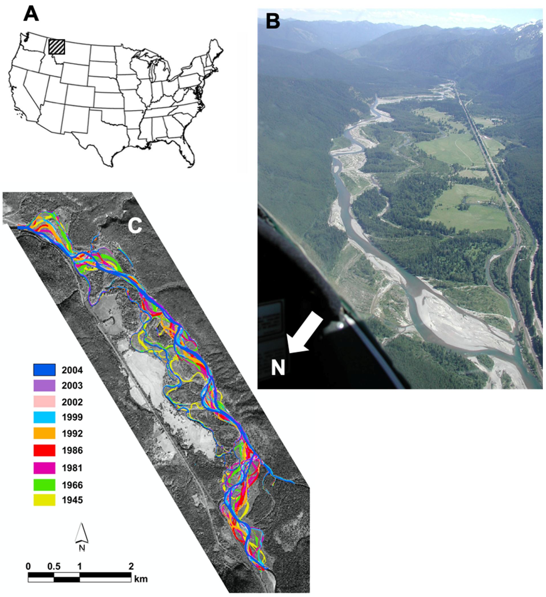
We conducted our remote sensing studies and method developments on the Nyack floodplain, an approximately 12 km long by 2 km wide alluvial reach of the Middle Fork of the Flathead River in northwestern Montana, USA (Figure 1A). Headwaters of the Middle Fork originate in the Bob Marshall–Great Bear Wilderness complex of Montana. At the site of the Nyack floodplain the river is an unregulated, natural flowing Horton–Strahler fifth-order river with Glacier National Park along the northeast boundary of the river with a combination of national forest and private lands along the southwest side of the river channel and occupying approximately 80% of the floodplain (Figure 1B). The Nyack floodplain is an alluvium-filled basin with a maximum depth to bedrock of ~150 m. Bedrock approaches the surface along the longitudinal gradient of the river, producing confined river reaches above and below the floodplain with distinct bedrock controlled knickpoints at both the upper and lower ends of the floodplain. The hydrologic regime is snowmelt dominated with maximum discharge generally occurring in May and June. Bankfull discharge is achieved at approximately 450–500 m3/s. Summer base flow is generally 30–50 m3/s. High discharge flooding events have been linked to PDO effects on regional climate and weather (Figure 1C) that drive the dynamic character embodied in the shifting habitat mosaic [7].
Figure 1.
(A) Map of United States showing location of Nyack floodplain of the Flathead River in western Montana. (B) Oblique aerial photograph of the Nyack floodplain looking toward the upper end of the floodplain at the top of the photo. Glacier National Park is at the left side of the river in this photo and the national forest and private lands are to the right side of the river. The river departs the floodplain in the lower right corner of the photo. (C) Quickbird satellite image of the Nyack floodplain with superimposed channel locations across nine years from 1945 to 2002 (modified from Whited et al. (2007) [48]).

Forest vegetation throughout the majority of the floodplain consists of black cottonwood (Populus trichocarpa), Engelman spruce (Picea engelmannii), Douglas fir (Pseudotsuga menziesii), western larch (Larix occidentalis), grand fir (Abies grandis), and fewer western hemlock (Tsuga heterophylla) and western red cedar (Thuja plicata). Shrub species are mainly willow (Salix spp.), alder (Alnus incana), hawthorn (Crataegus spp.), and dogwood (Cornus stolonifera).
The floodplain parafluvial zone is dominated by cobble scoured during annual flooding and point bars and island development. The largest cobble size is ~20 cm with most frequent cobble in the 5–10 cm range. Large wood, captured from the riparian floodplain forest as living trees, is transported by the river resulting in stranding on cobble bars and occasionally piled into aggregated log jams. Individual logs can often cause the flow to scour the river bed near the root wads with the deposition of fine gravel, sand, and silt behind the scour zones [8]. Cottonwood seedlings, willow, and alder are the primary woody species that colonize the cobble bars and islands, forming patches of vegetation that are either re-scoured or begin the process of “terrestrialization” that initiates succession toward orthofluvial zone development. The orthofluvial zone is characterized by a maturing riparian forest dominated by cottonwood and spruce. The presence of large vegetation in the orthofluvial results in fine sand and silt being deposited during floods as the large vegetation provides flow resistance. Old growth forest on the floodplain contains very old (>300 years) cottonwood, spruce, larch, and pine. The orthofluvial zone is frequently intersected by paleochannels (i.e., decade- to centuries-old abandoned channels) derived from the legacy of past flooding events, cut and fill alluviation, and channel avulsion [8].
3. Remote Sensing Acquisition
3.1. Airborne Light Detection and Ranging
LIDAR data were acquired in cooperation with the National Center for Airborne Laser Mapping (NCALM). Data were collected using an Optech ALTM (Airborne Laser terrain Mapper). This system uses a laser beam pulsing at 33 KHz and is directed by a scanning mirror to record the time and amplitude of a laser pulse reflected off target surfaces. Terrasolid TerraScan Lidar processing software was used by NCALM to process the raw LIDAR data and provide us with an unfiltered (i.e., first return) digital elevation model gridded to 1 m, as well as a 1 m filtered (i.e., bare earth) DEM. A relative elevation grid of the floodplain surface was derived from the bare earth DEM to estimate elevations above the water surface. The water surface and its associated elevation were extracted from the DEM to create the relative elevation grid. These elevations were then interpolated across the entire floodplain to create a water surface elevation grid. This floodplain water surface elevation grid was then subtracted from the bare earth DEM to produce the relative elevation grid. A vegetation canopy DEM to estimate plot-level tree heights [49] was calculated as the difference between the bare earth DEM and the first return LIDAR data.
3.2. Satellite Multispectral Imagery
Quickbird satellite imagery, consisting of four multispectral bands (blue—450 to 520 nm, green—520 to 600 nm, red—630 to 690 nm, NIR—760 to 900 nm) at a 2.4 m spatial resolution and a panchromatic band at a 0.6 m spatial resolution, was acquired for the Nyack floodplain. The image was orthorectified using a USGS 30 m DEM and several ground control points (GCPs) located throughout the floodplain.
3.3. Airborne Hyperspectral Imagery
We collected airborne hyperspectral data with an AISA hyperspectral imager from Spectral Imaging, Oulu, Finland. We deployed this imager from our own aircraft, a Cessna 185. Our research team developed all flight-mission engineering and imager deployments. The AISA system consists of a compact hyperspectral sensor head with digital data acquisition from 256 individual spectral wavebands (400 to 950 nm) and a Systron Donner C-MIGITS III GPS/INS sensor. A fiber-optic downwelling irradiance sensor (FODIS) is mounted to the upper exterior surface of the aircraft to obtain instantaneous irradiance for radiometric correction and conversion during post-processing of surface reflectance data. All data are synchronized and streamed to an onboard computer that controls the imager and stores the data. The fully programmable AISA system was configured to aggregate the spectral data into 20 bands at a frame collection rate cycle of 30 milliseconds. The aircraft with the AISA sensor was flown at 1000 m above ground level and at an approximate ground speed of 100 km/h. The AISA frame cycle rate and lens focal distance, combined with the altitude and ground speed, resulted in a pixel resolution of 1 m × 1 m. The hyperspectral data were collected along predetermined flight lines oriented along the long axis of the floodplain. Distance between flight lines was flown to produce a 40–50% overlap among all neighboring flight line images. Individual flight line data were initially rectified using Caligeo® software from Spectral Imaging. Final rectification and mosaicking were completed in ERDAS Imagine®. We used a combination of digital orthoquadrangle data (DOQs) and ground control points (GCPs) located throughout the floodplain to complete the orthorectification. Minor color-balancing between flight lines was applied during the mosaicking process. Imagery data were collected within a time period of 1.5 h at either side of solar noon. We selected the clearest day possible during autumn to achieve the maximum differentiation in leaf color between tree and shrub species, yet prior to leaf abscission and fall.
3.4. Airborne Ultra-High Resolution Multispectral Imagery
We collected ultra-high resolution digital photogrammetry (RGB) data using a standard professional digital camera (14.8 megapixel) mounted with a 50 mm lens. Images were collected simultaneously with the AISA hyperspectral data described above and have a pixel resolution at the floodplain surface of 5 cm × 5 cm. We used these images to assist in the classification of vegetation, river hydraulics, and georeferencing and mosaicking of the hyperspectral imaging. Images were rectified and mosaicked in ERDAS Imagine® using DOQs and GCPs.
3.5. Airborne Thermanl Imagery
We collected thermal data with an 8-bit digital thermal camera with video display and full frame 30 Hz capture rate. The camera was hardwired to an on-board computer to maximize data flow rate and provide direct, non-interference control of the camera. The camera was mounted on the pilot side wing strut ~2 m laterally from the aircraft fuselage and away from engine exhaust and radiant heat to minimize potential interference with the thermal imaging from flight operations.
4. Field Measures and Data Classification
4.1. River Hydraulics—Depth and Flow Velocity
We used a SonTek RS3000 Acoustic Doppler Velocity Profiler (ADP, SonTek/YSI, San Diego, CA, USA) to acquire detailed water depth and vertical profile flow velocity measurements within the main channel and off-channel habitats. We collected ADP data on eight separate dates ranging in river discharge from a minimum of 17 m3/s to a maximum discharge of 326 m3/s. The ADP uses three transducers generating 3 MHz acoustic pulse beams with different orientations relative to water flow. As the sound travels through the water, it is reflected in all directions by suspended particles transported with the flow. The energy from the sonar is most strongly reflected from the channel bottom, providing a measure of water depth. Energy reflected from advected particles suspended and moving with the river flow returns to the transducers with a frequency change referred to as a Doppler shift. Doppler shifts are linearly related to the velocity of the water. Data were recorded as the average water column velocity every 5 s. These data were augmented with a hand-held ADV (acoustic Doppler velocimeter) current meter for water depths <30 cm. The hand-held ADV was used exclusively in shallow waters (<30 cm) where the larger ADP cannot resolve velocity accurately.
We deployed the ADP from one of two watercraft, depending on river discharge. When the river discharge was >50 m3/s, the sonar head was attached to a 4.9 m whitewater catamaran and rowing frame. A rower and a sonar operator crewed the catamaran. When discharge was <50 m3/s, the ADP was deployed from a small 1 m × 0.5 m aluminum catamaran controlled by hand lines. The ADP was co-located with a Trimble AgGPS 132 v1.73 GPS receiver with one-meter positional accuracy. Data from the ADP and the GPS were streamed to a laptop computer on-board the large catamaran or to a shoreline operator by a FreeWave® wireless data transceiver (FreeWave Technologies, Inc. Boulder, CO, USA) from the handline-controlled catamaran. All data were time-stamped for later georeferencing of all depth and velocity profile measures. During data acquisition, the ADP was maneuvered through the channel and into various hydraulic conditions, from rapids and riffles to backwaters and glides, to obtain data from as complete an array of aquatic habitats, depths, and velocities as possible.
In classifying water depth and velocity, we processed the data through three steps: (1) the extraction of surface water features from the imagery, (2) the separation of off-channel from main channel waters, and (3) the classification of channel depth and flow velocities by statistical relationships established between spectral reflectance and the corresponding ground truth data from the ADP. Using the near-infrared band data from the Quickbird and a normalized difference vegetation index (NDVI), we conducted a supervised classification to isolate and extract water surfaces from surrounding land areas. This method depends on the relatively low near-infrared reflectance characteristics of water and the high sensitivity of the NDVI to photosynthetic biomasses to isolate open water surfaces from the surrounding landscape. The extracted water imagery was then converted from raster to vector format to distinguish main channel and off-channel habitats. Off-channel habitats had mud or sand/silt substrate and a unique spectral signature relative to the main channel, which was dominated by cobble substrate. Main and off-channel features were treated separately for classifying depth and flow characteristics measured in the field with the ADP.
Water depth of the now isolated water imagery was calculated using a linear transform model [50] that is widely used for estimating shallow water depth, including in-stream channels [51,52]. Using a small subset of the ADP data (120 points), a stepwise regression was applied to determine the best coherence between each spectral band and the observed water depth. A regression Equation (1) using three of four bands (green—X2, red—X3, NIR—X4) constructed from the data was applied to the entire image. The water depth was also aggregated into five depth categories (0–0.5, 0.5–1.0, 1.0–1.5, 1.5–2.0, and >2.0 m):
Water depth = −5.114 + ln(−4.563X2) + ln(−3.879X3) + ln(0.781X4)
We used an unsupervised clustering approach (ISODATA, iterative self-ordering data analysis, [53]) to enumerate similar clusters of spectral reflectances. The clusters were aggregated into four velocity categories (0–0.5, 0.5–1.0, 1.0–1.5, >1.5 m/s). A subset of the ADP data (677 points) was used to calibrate the classification relationship to spectral reflectance to assign the appropriate depth and velocity categories. The remaining ADP data were used to validate the relationship and assess the accuracy of the classification. This methodology followed the approach developed by Whited et al. [53,54] and Lorang et al. [55].
4.2. Surface Water–Ground Water Exchange and Groundwater Residence
In combination with other hydrogeological methods, tracer data can be used to better understand the hydrogeology of alluvial aquifer systems, especially near-surface groundwater flow paths. The inert noble gas radon, (i.e., the radioactive isotope 222Rn; half-life 3.8 days), emanates from rock surfaces into surrounding waters after the decay of 226Ra (emanation = recoil and diffusion; [56,57]) which is part of the radioactive decay series of naturally occurring uranium (238U). The solubility of radon in water is sufficiently high that it can be used as a groundwater tracer for determining the time a parcel of water has been in the subsurface as groundwater of river origin [58]. Surface waters usually contain very little radon unless they are receiving deep groundwater. During the recharge of aquifers, downwelling river water (i.e., infiltration of river water to groundwater) increases in radon activity as it flows in the subsurface. A constant radon activity concentration indicates that a steady-state concentration has been reached between isotope ingrowth and decay. For radon, about 90 percent of this steady state is reached after about 15 days.
Under plug-flow conditions, the law of radioactive ingrowth governs the radon activity dissolved in the water. The radon water age, calculated in Equation (2), is under plug-flow conditions using the radon activity concentrations of a sample (At) and at steady state (A∞ see, [58]), and adapted to the more general case of a non-zero initial activity, A0:
where λ = T1/2/ln 2 = 0.182 d−1, the decay constant for 222Rn.
τ = −1/λ ln [(A∞ − At)/(A∞ − A0)]
Often, groundwaters of different residence times mix in aquifers. In the case of a binary mixing of very young groundwater (i.e., recently infiltrated river water) with older groundwater, the residence time of the young water component can only be assessed with radon, if the actual mixing ratio is known. Nonetheless, elevated radon signals in surface waters provide direct proof of upwelling groundwater into these habitats, and the level of the radon signal gives an indication of both the upwelling intensity and the length of time the parcel of upwelling groundwater has been in the subsurface. Since outgassing of radon gas begins immediately when groundwater reaches the surface and is enhanced by the turbulent flow conditions in rivers and streams, the measurement of high radon concentrations in such waters indicates a high degree of connectivity to the groundwater.
We sampled surface waters, groundwaters from piezometers, groundwaters from deep wells, and groundwaters from upwelling discharge points within carefully excavated springs. Water was sampled from these diverse locations across the Nyack floodplain. Sampled water was captured in special bottles, closed without an atmospheric bubble, and returned to the laboratory for radon analysis on the same day. When piezometers or wells were sampled, small submersible pumps (positive displacement; Whale Superline 99, Munster Simms Eng. Ltd., Bangor, UK) were used to avoid placing the water under a vacuum, which would affect atmospheric pressure and degas the radon.
Radioactivity was measured as the number of decays per second, as Becquerel (bq), and the radioactivity concentration as bq/L. Radon was measured with a NITON Rad7-H2O instrument (Durridge Co., Bedford, MA, USA) counted as a measure of the 222Rn activity following standard procedures [59]. An α-spectrometric analysis is integrated in the instrument as a measure of the radon concentration in water (counting error 1σ, about ±10% at 10 bq/L; detection limit, about 0.2 bq/L).
4.3. Water Temperatures
To “ground truth” the thermal imager, we collected temperatures with a hand-held, field digital thermistor standardized to a laboratory-grade thermometer. Water temperatures were carefully obtained from waters within 1–2 cm from the surface. This requirement is because the airborne thermal imager can only collect thermal data from the water surface. Thermal data were carefully georeferenced in the field and then georectified with the airborne thermal imagery collected during the same solar and weather conditions taken the following day.
4.4. Periphyton and Chlorophyll
We collected periphyton along shorelines of the channel corresponding to the range in variation of attached algae growth near the water surface. In conjunction with the airborne hyperspectral imagery, periphyton samples were taken as 3 cm × 3 cm scapings from cobble surfaces, stored in whirl-packs, and placed on ice. Samples were georeferenced in the field and returned to the laboratory for standard chlorophyll analysis. Chlorophyll results were then referenced to the hyperspectral reflectance acquired from the georeferenced and mosaicked imagery.
4.5. Riparian Vegetation
The Nyack floodplain is partially characterized by wide-ranging patterns in the chronosequence of vegetation that results from processes leading to the development and maintenance of the shifting habitat mosaic [7]. We established a stratified random sampling design to observe vegetation colonization and development patterns associated with different landform features, from parafluvial lateral and mid-channel bars to orthofluvial shelves with old-growth forest. We sampled along the lateral floodplain dimension to provide a characterization of vegetation associated with major topographic features and spatially complex patches. We sampled on the longitudinal dimension of parafluvial islands and bars to observe responses of vegetation recruited to accreting surfaces. We also sampled along short transects across elevation gradients from orthofluvial shelves to the midpoint of orthofluvial paleochannels. Because landform features influence the site-specific ecology of plants, we sampled plant communities by major coverage categorization, which allowed analysis of variance in plant community metrics within landforms. Transects through large orthofluvial patches ranged up to several hundred meters in length, island and bar transects were generally much shorter (100–200 m), and transects across elevation gradients in the orthofluvial zones from shelves to paleochannels were generally < 50 m. All vegetation data were georeferenced with the satellite and airborne mosaicked imagery data.
5. Results and Discussion
5.1. LIDAR Bare Earth Model
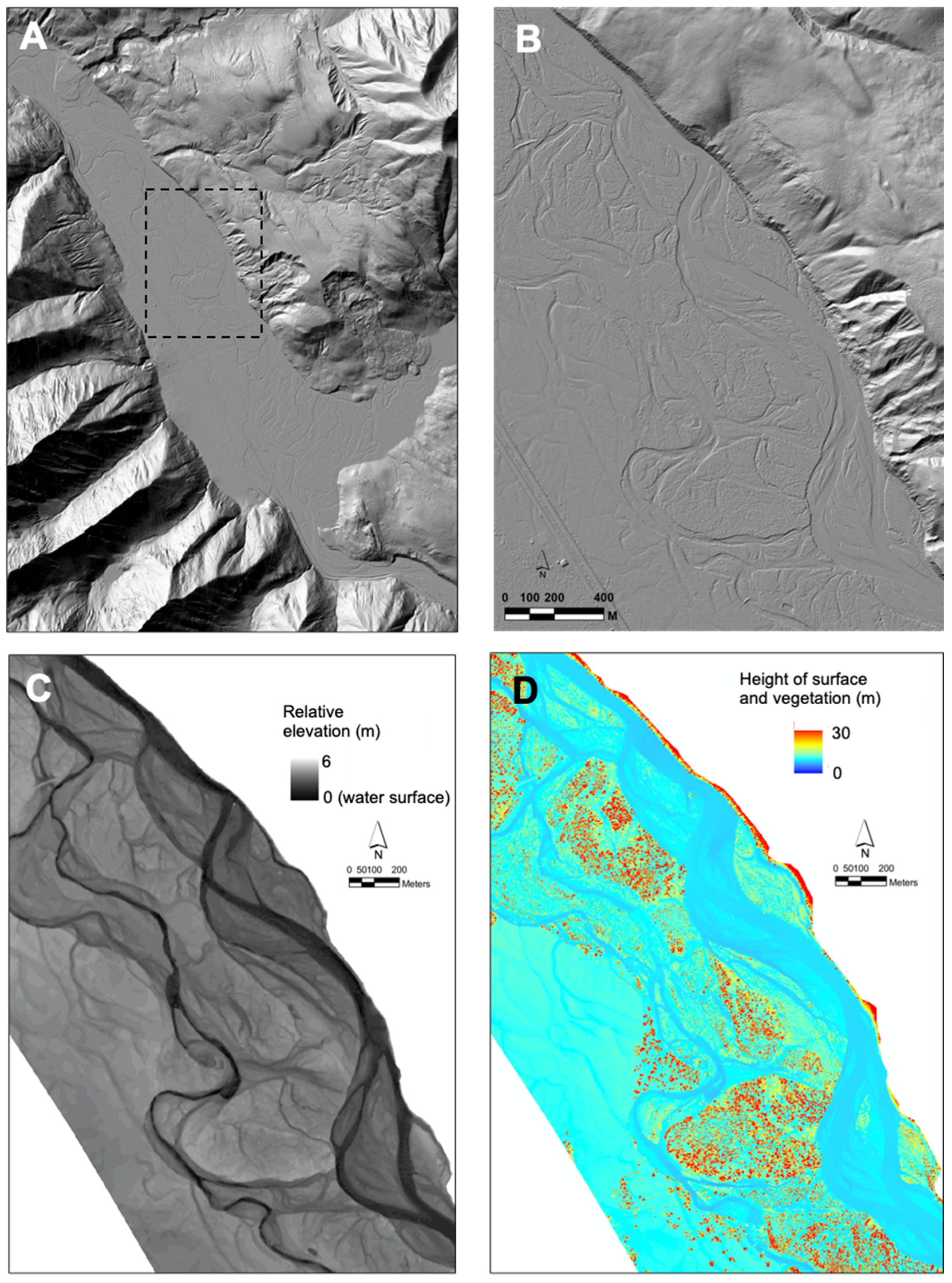
The bare earth DEM derived from the LIDAR data shows the basin geomorphology of the Nyack floodplain and surrounding hillslopes and valley form (Figure 2A,B). First- and second-order watersheds draining the mountains from the southwest and northeast of the floodplain are clearly observed. The relative elevations normalized to the water surface along the longitudinal gradient of the river (Figure 2C) illustrate current channels, recent channels, and older channels left as a legacy of cut and fill alluviation on the floodplain. These data, from both the bare earth model and the water surface corrected model, were used in conjunction with the satellite and airborne imagery to assess patterns of flow hydraulics, aquatic habitats, alluvial aquifer zones of preferential flow, and groundwater discharge. The first return DEM from the LIDAR data allowed us to describe riparian vegetation canopy heights and density (Figure 2D).
5.2. Aquatic Habitat Defined by Flow Velocity and Water Depth
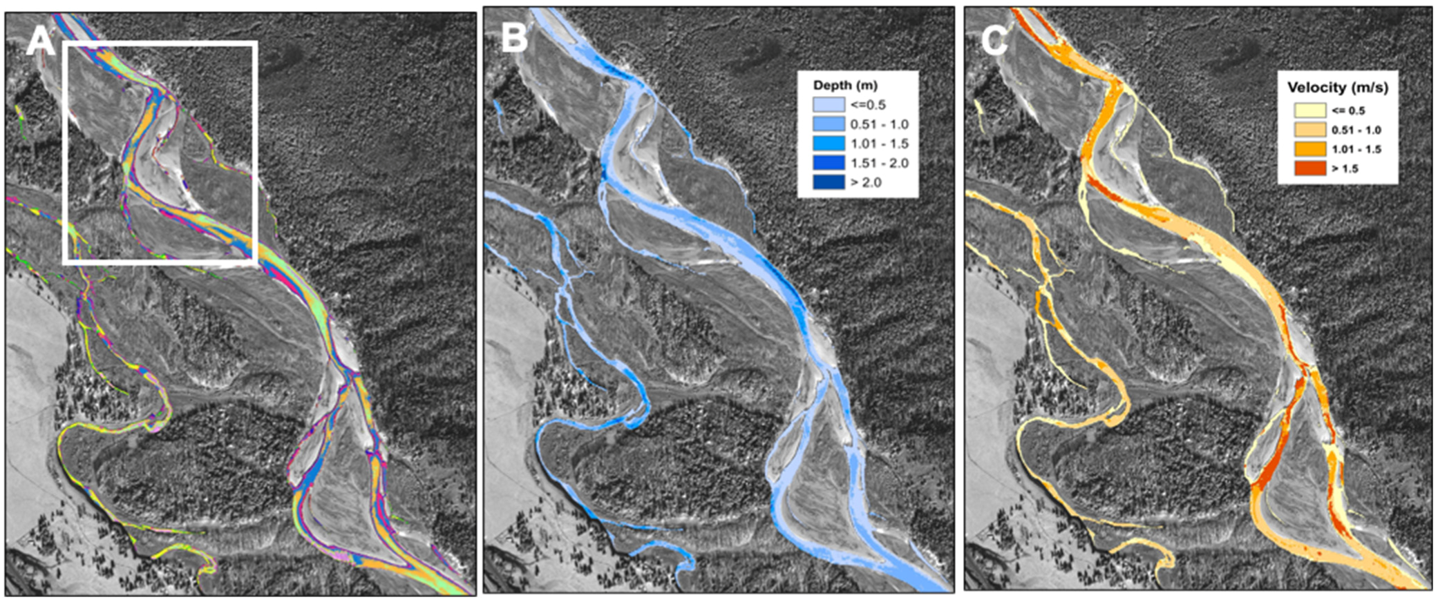
The water surface spectral reflectance patterns are directly related to surface water roughness and light absorption and reflectance characteristics of the water column. An unsupervised classification of the water body imagery (Figure 3A) was applied to differentiate flow categories within the main channel classification and then within the off-channel habitats. Linkage between field-measured flow and depth data with spectral reflectance data derived from the imagery sources was accomplished by using GPS locations to co-locate flow (Figure 3B) and depth (Figure 3C) with the spectral reflectance patterns of the water from pixels in the imagery that corresponded to those GPS locations. At the relatively coarse scale of the 12 km × 2 km floodplain, this was done using the Quickbird satellite imagery. When highly detailed analysis was desired, this was done using the high resolution airborne photogrammetric imagery.
Surface water roughness is a function of water depth, flow velocity, and bottom roughness, and hence is also related to the energetic state of the water column as defined by the Froude equation, a dimensionless number. For Froude values less than 1, the flow condition is referred to as sub-critical, and for values greater than 1, the flow is in a supercritical energetic condition that forces the water surface to break, forming a hydraulic jump to reduce the energy gradient by increasing the water depth. Likewise, the river can scour the bed to increase the depth until the flow reaches a subcritical condition. For this reason, supercritical flow typically only occurs in bedrock reaches and at specific channel locations rather than over broad areas. Using the depth and velocity data, we calculated Froude (Equation (3)) for each ADP data ensemble as
where V is the mean velocity, g is the acceleration due to gravity, and h is the water depth for each APD data ensemble located with GPS coordinates. As Froude values increase in a flow, the water surface becomes increasingly rough. High Froude (e.g., >0.8) values were observed in riffles and rapids. Very low Froude (e.g., <0.2) values were observed in pools and glides. Thus, the spectral reflectance directly due to river surface roughness captured by either the satellite or airborne photogrammetric imagery can be related to the Froude number as well as direct measures of depth and velocity. For habitat mapping, linking Froude to water surface roughness is a simple way to map the distribution of water depth and velocity together within an energetic context. When water is clear, which is often the case among cobble-bed rivers at low flow, the water color correlates closely with water depth. During the satellite Quickbird and airborne image acquisition, flow in the Flathead River on the Nyack floodplain was <50 m3/s, and water clarity was extremely high so that one could see the bottom to depths of up to 6 m except for areas where surface roughness limited depth perception. These same attributes of surface roughness and water clarity allow classification of flow velocity in much the same way one can visually recognize relative water velocity from still pictures. Linking ADP data to image pixels allows a much higher resolution of actual velocity bin intervals in the classification process.
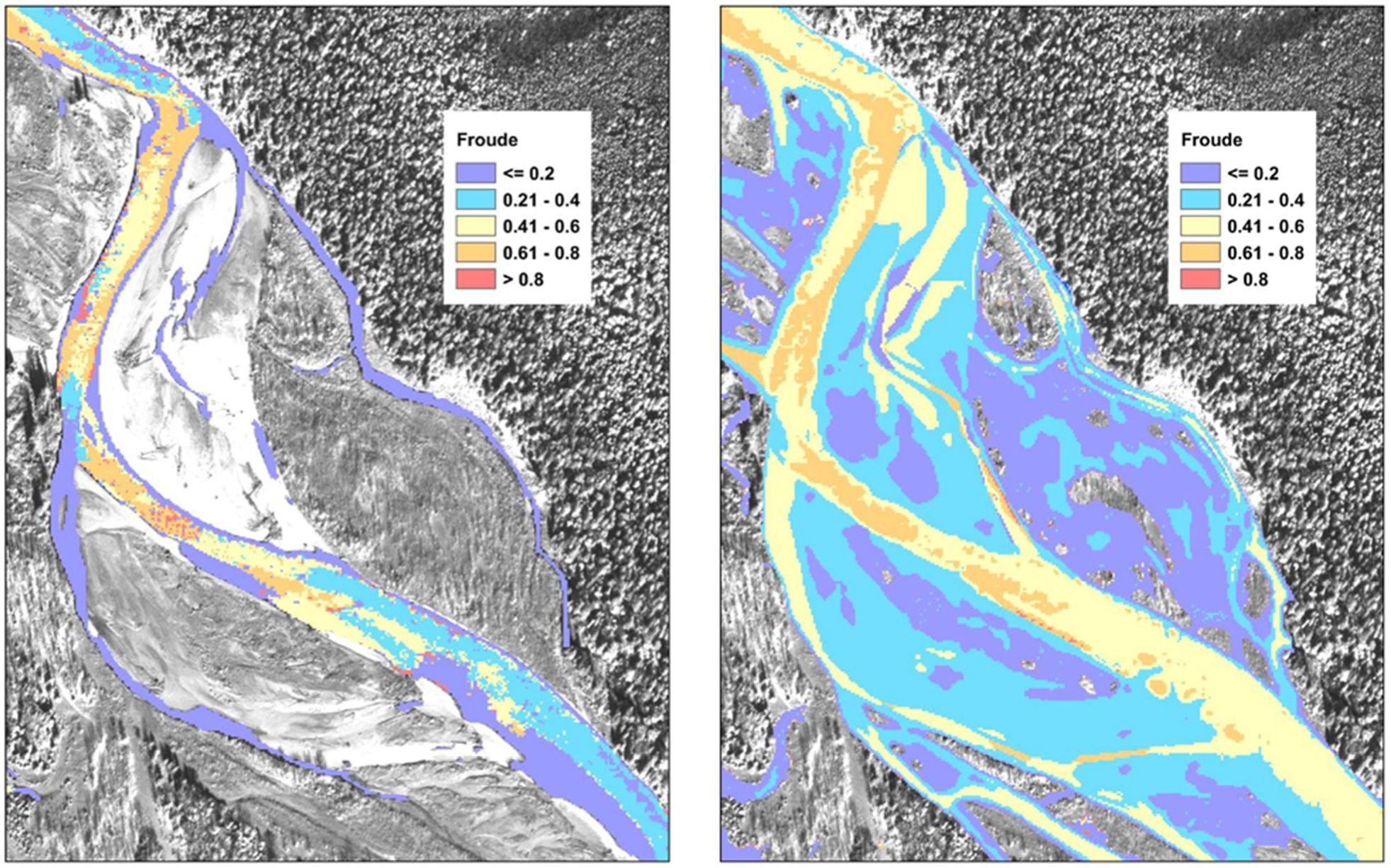
The relative elevation DEM developed from the LIDAR data (Figure 2C) was used to plot floodplain inundation and Froude from near baseflow (Figure 4 left panel; Q = 46 m3/s) to bankfull conditions (Figure 4 right panel; Q = 467 m3/s). Using a stage-discharge relationship based on the USGS gauge (12358500) located at West Glacier, Montana, we plotted floodplain inundation at 10 cm stage increments for the range of discharges from base flow to bankfull. In addition, flow velocity was plotted by establishing a basic relationship between velocity and river stage. Multiple measures of flow and depth developed this relationship at various discharge levels during the duration of our study. Estimates of flow velocity for the flooding scenarios were based on the initial velocity classification generated from the Quickbird satellite imagery. Only ADP data that were associated with the main channel environment were used to estimate velocity. ADP velocity data collected in backwaters and in off-channel environments were excluded, but we used depth of backwater and off-channel habitats when calculating incremental depths. Lorang et al. [60] provide a methodology to use the extensive ADP dataset to set upper limits of Froude. Velocity for any given pixel was then increased in the GIS modeling approach according to Equations (4) and (5) below, generated from the depth–velocity relationships measured in the ADP surveys. Equation (4) was used to simulate velocity for water depths > 0.8 m and Equation (5) was used for water depths < 0.8 m, where x is the water depth at a given stage.
y = 0.7754 ln(x) + 1.5088
y = 1.789(x) − 0.2042
After velocity was estimated for each stage, we set an upper limit on water velocity for each depth based on the threshold established by the ADP data for Froude given any depth [60]. For example, a depth of 1.5 m could not exceed a Froude number of 0.8. If the Froude number was greater than 0.8, the velocity was adjusted by recalculating velocity based on Froude and depth. Using 10 cm stage increments, we modeled depths and velocities to represent discharge regimes from 46 m3/s to 467 m3/s (i.e., base flow to bankfull). To check the accuracy of the estimated stage velocities and depths, the ADP surveys were done at two high discharges of 254 and 326 m3/s and used as reference data. We estimated the 254 m3/s discharge to correspond to a stage increase of 0.9 m from near baseflow conditions from the stage-discharge relationships. Using the depths and velocities that were estimated at the 0.9 m stage increase, error matrices were generated from the appropriate ADP survey (i.e., the 254 m3/s survey) to validate the depth and velocity results. The overall accuracy of depth was 70 and 72% for the discharges of 254 and 326 m3/s, respectively.
5.3. Aquatic Habitat Classification
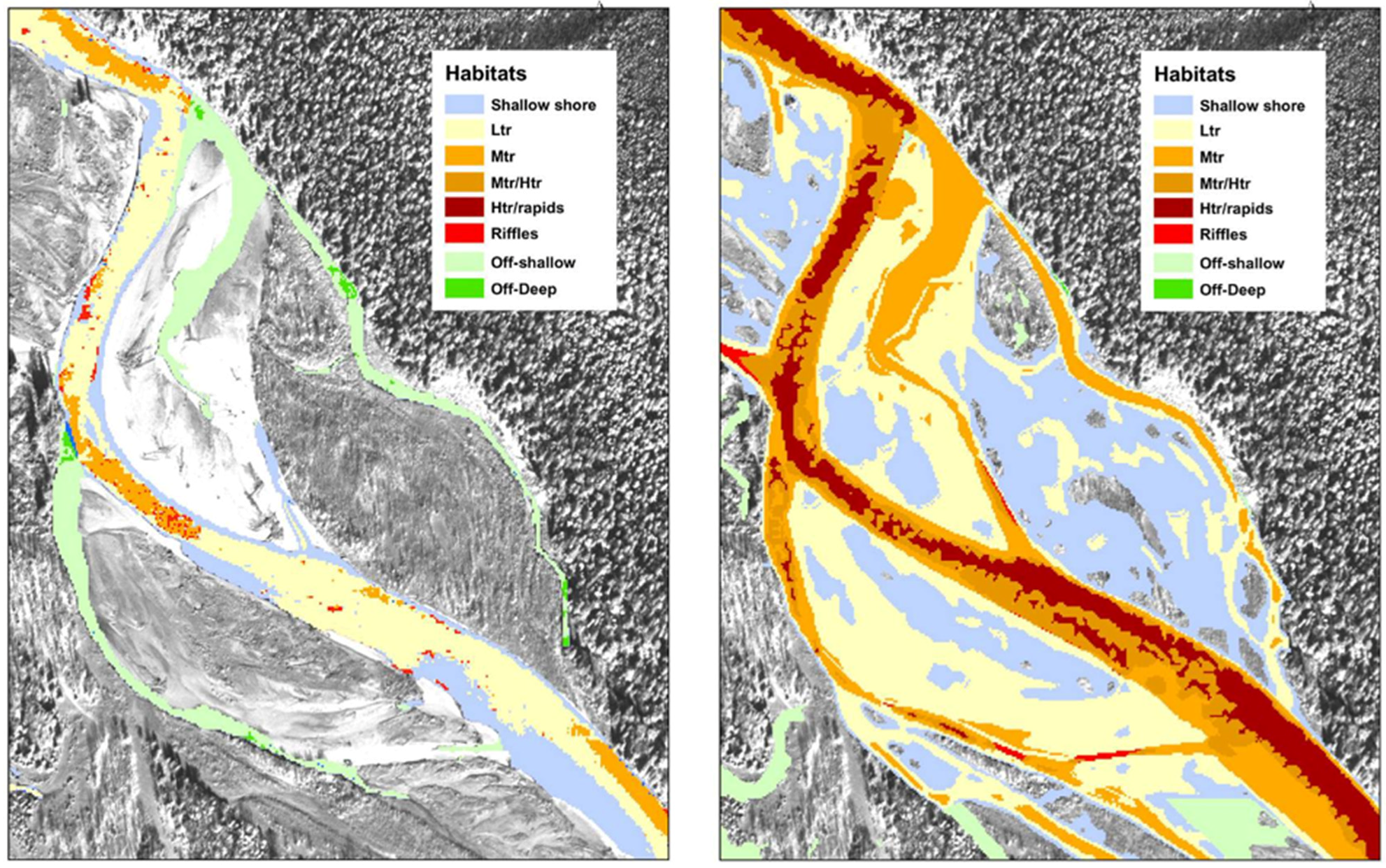
Despite the various potential sources of pixel-by-pixel error, we found the relationships between the field measures of flow velocity and depth to classified spectral reflectance of flow velocity and depth to be remarkably accurate. Slight differences between field measurements and GIS classification results were primarily associated with isolated pixels that were negligible at the scale of river channel hydraulics or at the scale that fish use the river. Using the spatial, pixel-by-pixel classifications of depth and velocity, we classified Froude number values to produce what we refer to as a “Froude space” distribution across all surfaces of the river channel (Figure 4). We then used the distribution of Froude, water depth, and channel position to aggregate pixels into patches and apply specific aquatic habitat designations (e.g., shallow shoreline, low turbulent runs, medium turbulent run, high turbulent run, riffles, off-channel deep pools, off channel shallow pools) at each of the two modeled discharges (Figure 5 left panel, right panel).
5.4. Ground Water–Surface Water Interaction, Water Temperature, and Periphyton
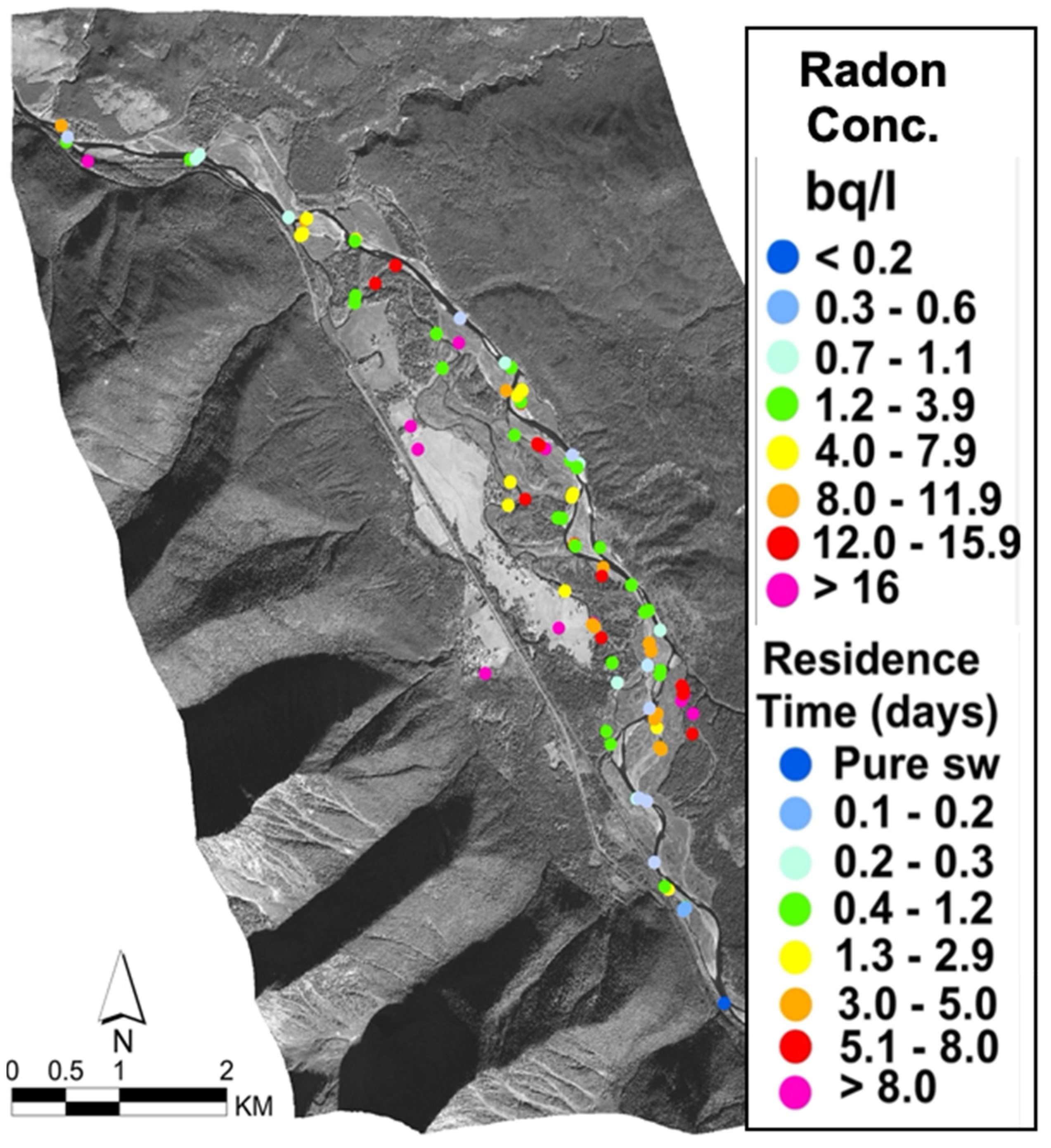
The radon tracer data showed high variation across the Nyack floodplain (Figure 6). Near-zero radon concentrations were only observed in surface water collected at the upstream end of the floodplain before it entered the alluvial reach. This indicates that there was little groundwater discharge into the main channel at the head of the floodplain, as waters passed through confined river reaches upstream of the geomorphic knickpoint at the head of the floodplain. Further, radon that may have been added above the floodplain had experienced out-gassing insufficient to remove the radon from channel waters. ADP discharge measurements in the river along the length of the floodplain revealed losses and gains of up to 30% of the total discharge rate (see [7]). Radon measurements confirm these patterns, particularly at the downstream ends of gravel bars where large-scale groundwater discharge from the alluvial aquifer appearing as upwelling could be visibly observed and sampled, and radon concentrations measured. A springbrook that occurs along the southwest side of the main channel occupying a paleochannel is continually fed by upwelling groundwater. Water sampled from piezometers inserted at the upstream (downwelling) ends of gravel bars generally had lower radon concentrations, particularly within the parafluvial zone of the floodplain, thus showing high subsurface flow rates of as much as 300 m per day and residence times of as little as a few hours hundreds of meters from the river (Figure 6). These values for groundwater flow velocity are extraordinarily high and illustrate high surface water–groundwater exchange rates and extremely high hydraulic conductivity in the Nyack floodplain.
Radon tracer data has inherent variation. Thus, the “age” of near-surface groundwater can only be estimated because recently infiltrated surface waters that are recent groundwaters with a low concentration of radon may mix with waters of longer residence times with the maximum concentration of radon. Groundwaters may also experience outgassing of radon as they approach the surface. Finally, radon concentration reaches a steady state after about 3–4 weeks due to radon’s short radioactive half-life. These sources of variation nonetheless provide a clear indication of the degree of connectivity to the groundwater and a better understanding of the physico-chemical characteristics, such as nutrient availability or temperature regimes, associated with habitats receiving groundwater discharge.
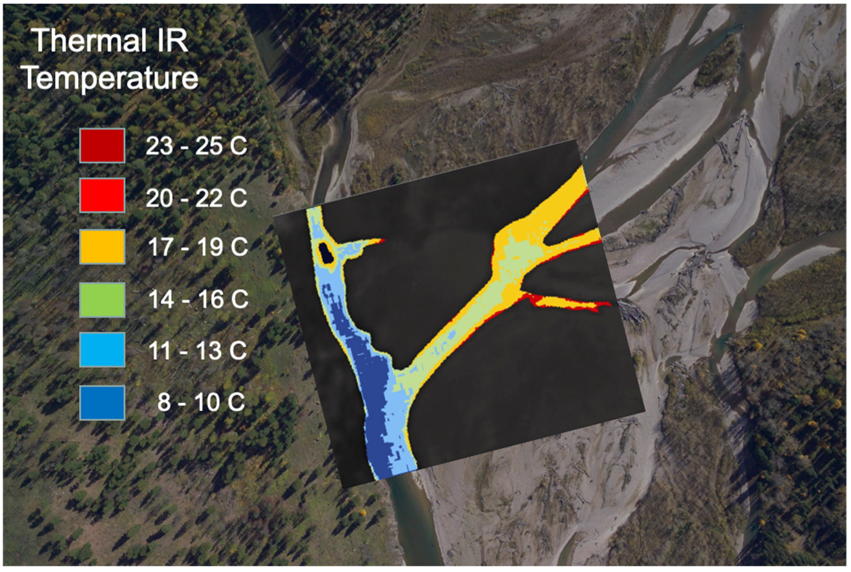
Our radon data corresponded well with the airborne thermal imaging data, which illustrate a high variation in channel and off-channel habitats warmed by solar radiation, but simultaneously cooled by groundwater discharging into surface waters including the main channel, gravel bar springs, springbrooks, and both parafluvial and orthofluvial ponds. In the thermal imagery (Figure 7), we observe shorelines and main channel habitats being significantly cooled by groundwater discharge at the downstream end of a large gravel bar. These data can be extended to explain why ponds with little or no groundwater connectivity will become very warm in summer and freeze completely top to bottom in winter, while ponds with a high flow-through of groundwater stay cool in summer and remain open and “steamy” in winter [11,61]. The high variation in water temperature is extremely important in the support of floodplain biodiversity of aquatic, semi-aquatic, avian, and mammalian species [3].
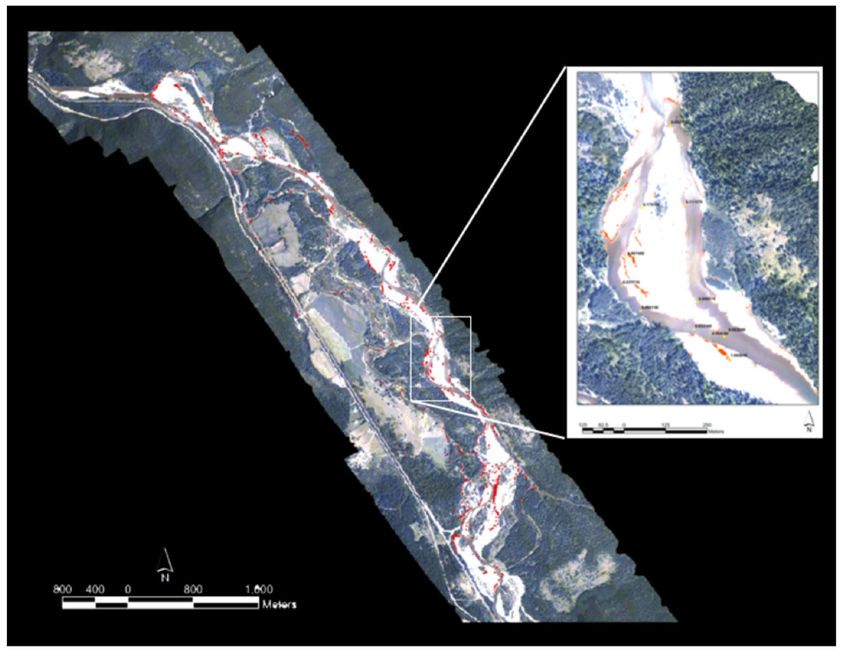
Surface water recharge (i.e., downwelling river water) carries organic matter from the surface into the alluvial aquifer. Subsurface decomposition of this organic matter affects oxygen concentrations [62] and the release of plant growth nutrients (e.g., phosphates, nitrates), which can be taken up by the epiphytic algae [11,63] and create localized “hot spots” of primary productivity in an otherwise nutrient-poor environment. We measured enhanced primary productivity and co-registered these data with the airborne hyperspectral imagery (Figure 8). These data show a high coherence between the georeferenced radon data, airborne thermal imaging data, and the sites of intensive algal growth. Thus, radon signals and thermal imagery data demonstrate that a rich and complex array of hydrological exchange and mixing processes occur all across the Nyack floodplain, resulting in a diverse mosaic of aquatic habitats with differing physico-chemical and productivity characteristics.
5.5. Classification of Vegetation and Riparian Patches
We used a combination of the Quickbird satellite multispectral imagery, airborne hyperspectral imagery, and the LIDAR data to produce a detailed vegetation and land cover map for the Nyack floodplain. An unsupervised classification employing ERDAS was generated from the satellite Quickbird image using the four multispectral bands and NDVI (Normalized Differential Vegetation Index) to identify six general cover types; water, cobble, coniferous trees, deciduous trees, grasslands, and agricultural pasture. The hyperspectral image data were used to differentiate reflectance characteristics within the deciduous vegetation classification. Using ENVI 3.5 (RSI 2005), spectral signatures were generated from known ground truth plots among the dominant deciduous community types. Using the mean spectral signature for the deciduous cover types, the mixture-tuned matched filtering (MTMF) was used to classify the deciduous vegetation into its major constituents of cottonwood, willow, or alder. Image classification accuracy evaluation corresponded with field species identification >95%.
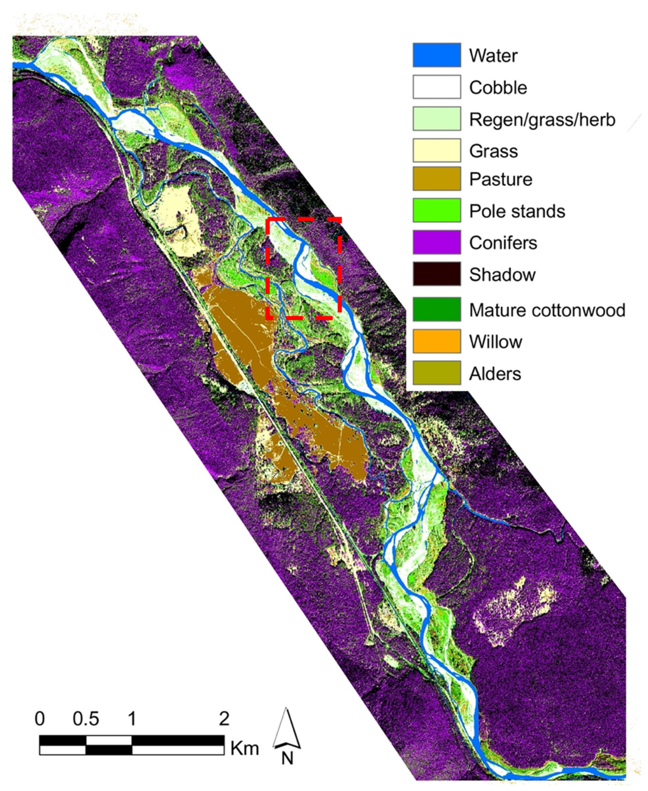
The LIDAR data were used to further differentiate age categories of the cottonwood. Among the pixels classified as cottonwood, we determined canopy height as the difference between the bare earth DEM and the first return DEM. Pixels classified as cottonwood with a bare earth DEM to first return DEM differential of >10 m were classified as mature cottonwoods, between 1.5 and 10 m were identified as pole stand cottonwood, and patches less than 1.5 m in height were classified as regeneration cottonwood patches. Taking this approach, we were able to classify the vegetation across the entire floodplain at a 1 × 1 m pixel resolution and differentiate not only between major species (e.g., spruce, cottonwood, willow, alder), but also within species age stands of cottonwood, the dominant gallery forest species (Figure 9).
Tree species succession on the Nyack floodplain begins as a mix of cottonwood, willow, and alder. As the patch matures, cottonwood eventually captures the canopy; thus, willow is rarely found on orthofluvial cottonwood patches and alder becomes restricted to edges of paleochannels intersecting the older mature cottonwood stands. We were unable to remotely sense early size or age classes of spruce, larch, or Douglas fir, because these species almost exclusively appear as understory species in 30–50-year-old cottonwood stands and thus are generally obscured from aerial view by the mature cottonwood gallery. However, these species, especially spruce, enter the upper mature forest canopy and eventually (>80 years) can be distinguished from the cottonwood. As the floodplain forest matures, spruce eventually replaces cottonwood on very old (>200 years) surfaces in the orthofluvial zone.
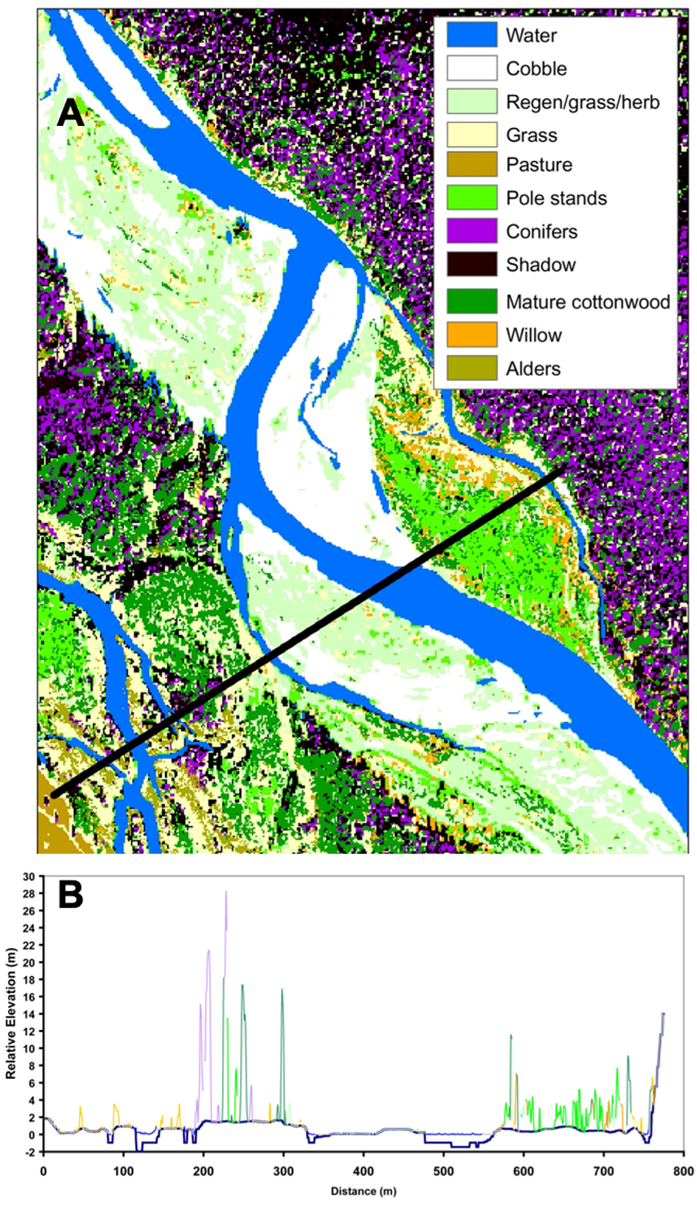
The species level classification of the remotely sensed hyperspectral data, when geospatially linked with the bare earth DEM and the three-dimensional LIDAR canopy height data (shown above in Figure 2D), permitted a more detailed analysis of the floodplain vegetation and processes (Figure 10). For example, the coupling of LIDAR and hyperspectral data allowed us to create virtual transects through the floodplain for the analysis of tree canopy height coupled with specific species and floodplain elevations (Figure 10B).
6. Conclusions
Remote sensing has broad application in river ecology, hydrology, fish biology, and the conservation and management of large rivers and floodplains. In this paper, we have shown how these remote sensing tools, coupled with detailed field measures, provide great detail of critical within-channel and off-channel floodplain attributes among even the most highly complex anastomosing and braided gravel-bed river floodplains.
- We have shown that linking of Quickbird satellite imagery (multispectral at a 2.4 m spatial resolution and panchromatic at a 0.6 m spatial resolution) with airborne LIDAR (to be employed for measuring river depth and velocity) and the detailed determination and quantification of aquatic habitats results in an extremely high resolution of river hydraulics.
- The coupling of remote sensing data permits high resolution classification and modeling based on the direct relationship of spectral reflectance to measured depth and velocity. Because this approach is not dependent upon resolving complex flow algorithms that poorly resemble the true complexity of river hydraulics, this approach provides the researcher with subtle habitat characteristics at scales used by aquatic organisms, especially migratory fish.
- Hyperspectral imaging, focusing on channel shorelines, coupled with thermal imaging and detailed temperature and naturally occurring radon tracer data provides important insight into groundwater–surface water interactions. When integrated, these data illustrate sites of potential nutrient upwelling from groundwater discharging into shallow channel shorelines and springs, including diverse and complex aquatic habitats. These data reveal the spatial complexity of aquatic temperature regimes across these habitats and locations where “hot-spots” of epiphytic algal growth affect river primary and secondary productivity and support of floodplain biodiversity.
- The coupling of satellite multispectral imaging, airborne hyperspectral imaging, and LIDAR bare earth and vegetation DEMs permits the identification of floodplain vegetation across serial stages from regeneration through old growth. These data allow the resolution of floodplain forest species and measure the topography, forest canopy height, and complex structure of the vegetation (e.g., differentiation of dominant tree species by canopy height and age class). This also facilitates answers to more complex questions related to spatial patterns of vegetation development, the incorporation of large wood into the river channel, and the distribution and abundance of main channel and off-channel linkages of aquatic and terrestrial habitats.
River floodplains are among the most globally threatened ecosystems [4,64]. The threats to ecosystem integrity are due to river regulation downstream of dams, inundation upstream of dams, disruption in connectivity along stream corridors, modification of hydrologic regimes, and geomorphic processes. Other human activities such as agricultural and urban encroachment, transportation corridors, and stabilizing river banks with levees and hardening structures to attempt control of flooding events all disrupt natural river processes. Remote sensing tools, as we have described herein, can be used to determine the spatial and temporal linkages within large, alluvial river systems, including natural characteristics of the exchange of water and materials along with longitudinal connections from streams to rivers, lateral connections between river and floodplain systems, and vertical surface and subsurface water exchanges. Remote sensing imagery coupled with georeferenced supporting data can illustrate hydrogeomorphic processes, driven by river power and cut and fill alluviation, the extent of dynamics in floodplain landscapes, and the characteristics of river structure and function that foster ecosystem complexity, resulting in a high diversity of habitats and a high biodiversity at local and regional scales.
Author Contributions
Conceptualization, F.R.H., M.S.L., and T.G.; methodology, F.R.H., M.S.L., and T.G.; image validation, F.R.H., M.S.L., and T.G.; analysis, F.R.H., M.S.L., and T.G.; data curation, F.R.H., M.S.L., and T.G.; writing—original draft preparation, F.R.H., M.S.L., and T.G.; writing—review and editing, F.R.H., M.S.L., and T.G. All authors have read and agreed to the published version of the manuscript.
Funding
This research, including the method development, approach, data acquisition and processing, instrumentation, and remote sensing, was funded by a variety of sources, including the National Science Foundation, US Bureau of Reclamation, US Park Service, and private foundations.
Institutional Review Board Statement
Not Application.
Informed Consent Statement
Not Application.
Data Availability Statement
Not Application.
Acknowledgments
We thank D.C. Whited and P.L. Matson for both field and laboratory assistance and data processing.
Conflicts of Interest
The authors declare no conflict of interest. The funders had no role in the design of the study; in the collection, analyses, or interpretation of data; in the writing of the manuscript, or in the decision to publish the results.
References
- Naiman, R.J.; Decamps, H.; Pollock, M. The role of riparian corridors in maintaining regional biodiversity. Ecol. Appl. 1993, 3, 209–212. [Google Scholar] [CrossRef] [PubMed]
- Ward, J.V. An expansive perspective of riverine landscapes: Pattern and process across scales. GAIA-Ecol. Perspect. Sci. Soc. 1997, 6, 52–60. [Google Scholar] [CrossRef]
- Hauer, F.R.; Locke, H.; Dreitz, V.J.; Hebblewhite, M.; Lowe, W.H.; Muhlfeld, C.C.; Nelson, C.R.; Proctor, M.F.; Rood, S.B. Gravel-bed river floodplains are the ecological nexus of glaciated mountain landscapes. Sci. Adv. 2016, 2, e1600026. [Google Scholar] [CrossRef] [PubMed] [Green Version]
- Tockner, K.; Stanford, J.A. Riverine flood plains: Present state and future trends. Environ. Conserv. 2002, 29, 308–330. [Google Scholar] [CrossRef] [Green Version]
- Tockner, K.; Pusch, M.; Borchardt, D.; Lorang, M.S. Multiple stressors in coupled river-floodplain ecosystems. Freshw. Biol. 2010, 55, 135–151. [Google Scholar] [CrossRef]
- Likens, G.E.; Bormann, F.H. Linkages between terrestrial and aquatic ecosystems. BioScience 1974, 24, 447–456. [Google Scholar] [CrossRef]
- Stanford, J.A.; Lorang, M.S.; Hauer, F.R. The Shifting Habitat Mosaic of River Ecosystems. Verh. Int. Ver. Theor. Angew. Limnol. 2005, 29, 123–136. [Google Scholar] [CrossRef]
- Lorang, M.S.; Hauer, F.R. Fluvial Geomorphic Processes. In Methods in Stream Ecology—Volume 1: Ecosystem Structure, 3rd ed.; Hauer, F.R., Lamberti, G.A., Eds.; Academic Press/Elsevier: New York, NY, USA, 2017; pp. 89–107. [Google Scholar]
- Stanford, J.A.; Ward, J.V. An ecosystem perspective of alluvial rivers: Connectivity and the hyporheic corridor. J. N. Am. Benthol. Soc. 1993, 12, 48–60. [Google Scholar] [CrossRef]
- Woessner, W.W. Hyporheic Zones. In Methods in Stream Ecology—Volume 1: Ecosystem Structure, 3rd ed.; Hauer, F.R., Lamberti, G.A., Eds.; Academic Press/Elsevier: New York, NY, USA, 2017; pp. 129–157. [Google Scholar]
- Brunke, M.; Gonser, T. The ecological significance of exchange processes between rivers and groundwater. Freshw. Biol. 1997, 37, 1–33. [Google Scholar] [CrossRef] [Green Version]
- Mahoney, J.M.; Rood, S.B. Streamflow requirements for cottonwood seedling recruitment—An integrative model. Wetlands 1998, 18, 634–645. [Google Scholar] [CrossRef]
- Kleindl, W.J.; Rains, M.C.; Marshall, L.A.; Hauer, F.R. Fire and flood expand the floodplain shifting habitat mosaic concept. Freshw. Sci. 2015, 34, 1366–1382. [Google Scholar] [CrossRef] [Green Version]
- Peipoch, M.; Brauns, M.; Hauer, F.R.; Weitere, M.; Valett, H.M. Ecological simplification: Influences on riverscape complexity. BioScience 2015, 65, 1057–1065. [Google Scholar] [CrossRef] [Green Version]
- Durand, M.; Gleason, C.; Garambois, P.A.; Bjerklie, D.; Smith, L.; Roux, H.; Rodriguez, E.; Bates, P.D.; Pavelsky, T.M.; Monnier, J. An intercomparison of remote sensing river discharge estimation algorithms from measurements of river height, width, and slope. Water Resour. Res. 2016, 52, 4527–4549. [Google Scholar] [CrossRef] [Green Version]
- Hubbart, J.A.; Kellner, E.; Kinder, P.; Stephan, K. Challenges in aquatic physical habitat assessment: Improving conservation and restoration decisions for contemporary watersheds. Challenges 2017, 8, 31. [Google Scholar] [CrossRef] [Green Version]
- Frechette, D.M.; Dugdale, S.; Dodson, J.; Bergeron, N. Understanding summertime thermal refuge 1033 use by adult Atlantic salmon using remote sensing, river temperature monitoring, and acoustic telemetry. Can. J. Fish. Aquat. Sci. 2018, 75, 1999–2010. [Google Scholar] [CrossRef]
- Kasvi, E.; Salmela, J.; Lotsari, E.; Kumpula, T.; Lane, S. Comparison of remote sensing based approaches for mapping bathymetry of shallow, clear water rivers. Geomorphology 2019, 333, 180–197. [Google Scholar] [CrossRef]
- Guénard, G.; Morin, J.; Matte, P.; Secretan, Y.; Valiquette, E.; Mingelbier, M. Deep learning habitat modeling for moving organisms in rapidly changing estuarine environments: A case of two fishes. Estuar. Coast. Shelf Sci. 2020, 238, 106713. [Google Scholar] [CrossRef]
- Piégay, H.; Arnaud, F.; Belletti, B.; Bertrand, M.; Bizzi, S.; Carbonneau, P.; Dufour, S.; Liébault, F.; Ruiz-Villanueva, V.; Slater, L. Remotely sensed rivers in the Anthropocene: State of the art and prospects. Earth Surf. Processes Landf. 2020, 45, 157–188. [Google Scholar] [CrossRef]
- Hankin, D.G.; Reeves, G.H. Estimating total fish abundance and total habitat area in small streams based on visual estimation methods. Can. J. Fish. Aquat. Sci. 1988, 45, 834–844. [Google Scholar] [CrossRef]
- Roper, B.B.; Scarnecchia, D.L. Observer variability in classifying habitat types in stream surveys. N. Am. J. Fish. Manag. 1995, 15, 49–53. [Google Scholar] [CrossRef] [Green Version]
- Thompson, W.L. Hankin and Reeves’ Approach to Estimating Fish Abundance in Small Streams: Limitations and Alternatives. Trans. Am. Fish. Soc. 2003, 132, 69–75. [Google Scholar] [CrossRef]
- Gore, J.A.; Judy, R.D., Jr. Predictive models of benthic macroinvertebrate density for use in instream flow studies and regulated flow management. Can. J. Fish. Aquat. Sci. 1981, 38, 1363–1370. [Google Scholar] [CrossRef]
- Gallagher, S.P.; Gard, M.F. Relationship between chinook salmon (Oncorhynchus tshawytscha) redd densities and PHABSIM-predicted habitat in the Merced and Lower American rivers, California. Can. J. Fish. Aquat. Sci. 1999, 56, 570–577. [Google Scholar] [CrossRef]
- Spence, R.; Hickley, P. The use of PHABSIM in the management of water resources and fisheries in England and Wales. Ecol. Eng. 2000, 16, 153–158. [Google Scholar] [CrossRef]
- Shirvell, C.S. Ability of PHABSIM to predict chinook salmon spawning habitat. Regul. Rivers Res. Manag. 1989, 3, 277–289. [Google Scholar] [CrossRef]
- Bourgeois, G.; Cunjak, R.A.; Caissie, D. A spatial and temporal evaluation of PHABSIM in relation to measured density of juvenile Atlantic salmon in a small stream. N. Am. J. Fish. Manag. 1998, 16, 154–166. [Google Scholar] [CrossRef]
- Put, W.; Pasture, P. Don’t throw out the baby (PHABSIM) with the bathwater: Bringing scientific credibility to use of hydraulic habitat models, specifically PHABSIM. Future of Salmon in the Face of Change. Fisheries 2017, 146, 493–560. [Google Scholar]
- Leclerc, M.; Boudreault, A.; Bechara, J.A.; Corfa, G. Two-dimensional hydrodynamic modeling: A neglected tool in the instream flow incremental methodology. Trans. Am. Fish. Soc. 1995, 124, 645–662. [Google Scholar] [CrossRef]
- Ghanem, A.; Steffler, P.; Hicks, F.; Katopodis, C. 2-D hydraulic simulation of physical conditions in flowing streams. Regul. Rivers Res. Manag. 1996, 12, 185–200. [Google Scholar] [CrossRef]
- Kondolf, G.M.; Larsen, E.W.; Williams, J.G. Measuring and modeling the hydraulic environment for assessing instream flows. N. Am. J. Fish. Manag. 2000, 20, 1016–1028. [Google Scholar] [CrossRef]
- Lorang, M.S.; Tonolla, D. Combining active and passive hydroacoustic techniques during flood events for rapid spatial mapping of bedload transport patterns in gravel-bed rivers. Fundam. Appl. Limnol. 2014, 184, 231–246. [Google Scholar] [CrossRef]
- Marotz, B.; Lorang, M.S. Pallid sturgeon larvae: The drift dispersion hypothesis. J. Appl. Ichthyol. 2018, 34, 373–381. [Google Scholar] [CrossRef]
- Mejia, F.H.; Torgersen, C.E.; Berntsen, E.K.; Maroney, J.R.; Connor, J.M.; Fullerton, A.H.; Ebersole, J.L.; Lorang, M.S. Longitudinal, Lateral, Vertical, and Temporal Thermal Heterogeneity in a Large Impounded River: Implications for Cold-Water Refuges. Remote Sens. 2020, 12, 1386. [Google Scholar] [CrossRef] [PubMed]
- Goodchild, M.F. Integrating GIS and remote sensing for vegetation analysis and modeling: Methodological issues. J. Veg. Sci. 1994, 5, 615–626. [Google Scholar] [CrossRef]
- Wulder, M.A.; Franklin, S.E.; White, J.C.; Linke, J.; Magnussen, S. An accuracy assessment framework for large-area land cover classification products derived from medium-resolution satellite data. Int. J. Remote Sens. 2006, 27, 663–683. [Google Scholar] [CrossRef]
- Broge, N.H.; Leblanc, E. Comparing prediction power and stability of broadband and hyperspectral vegetation indices for estimation of green leaf area index and canopy chlorophyll density. Remote Sens. Environ. 2000, 76, 156–172. [Google Scholar] [CrossRef]
- Cochrane, M.A. Using vegetation reflectance variability for species level classification of hyperspectral data. Int. J. Remote Sens. 2000, 21, 2075–2087. [Google Scholar] [CrossRef]
- Haboudane, D.; Miller, J.R.; Pattey, E.; Zarco-Tejada, P.J.; Strachan, I.B. Hyperspectral vegetation indices and novel algorithms for predicting green LAI of crop canopies: Modeling and validation in the context of precision agriculture. Remote Sens. Environ. 2004, 90, 337–352. [Google Scholar] [CrossRef]
- Underwood, E.; Ustin, S.; DiPietro, D. Mapping nonnative plants using hyperspectral imagery. Remote Sens. Environ. 2003, 86, 150–161. [Google Scholar] [CrossRef]
- Hirano, A.; Madden, M.; Welch, R. Hyperspectral image data for mapping wetland vegetation. Wetlands 2003, 23, 436–448. [Google Scholar] [CrossRef]
- Turner, W.; Spector, S.; Gardiner, N.; Fladeland, M.; Sterling, E.; Steininger, M. Remote sensing for biodiversity science and conservation. Trends Ecol. Evol. 2003, 18, 306–314. [Google Scholar] [CrossRef]
- Rugenski, A.T.; Minshall, G.W.; Hauer, F.R. Riparian Processes and Interactions. In Methods in Stream Ecology—Volume 2: Ecosystem Function, 3rd ed.; Lamberti, G.A., Hauer, F.R., Eds.; Academic Press/Elsevier: New York, NY, USA, 2017; pp. 83–111. [Google Scholar]
- Lefsky, M.A.; Cohen, W.B.; Parker, G.G.; Harding, D.J. Lidar remote sensing for ecosystem studies. BioScience 2002, 52, 19–30. [Google Scholar] [CrossRef]
- McKean, J.; Nagel, D.; Tonina, D.; Bailey, P.; Wright, C.W.; Bohn, C.; Nayegandhi, A. Remote sensing of channels and riparian zones with a narrow-beam aquatic-terrestrial LIDAR. Remote Sens. 2009, 1, 1065–1096. [Google Scholar] [CrossRef] [Green Version]
- Tockner, K.; Lorang, M.S.; Stanford, J.A. River flood plains are model ecosystems to test general hydrogeomorphic and ecological concepts. River Res. Appl. 2010, 26, 76–86. [Google Scholar] [CrossRef]
- Whited, D.C.; Lorang, M.S.; Harner, M.J.; Stanford, J.A.; Hauer, F.R.; Kimball, J.S. Climate, hydrologic disturbance, and succession: Drivers of floodplain pattern. Ecology 2007, 88, 940–953. [Google Scholar] [CrossRef] [Green Version]
- Popescu, S.C.; Wynne, R.H.; Nelson, R.F. Estimating plot-level tree heights with LIDAR: Local filtering with a canopy-height based variable window size. Comput. Electron. Agric. 2002, 37, 71–95. [Google Scholar] [CrossRef]
- Lyzenga, D.R. Passive remote-sensing techniques for mapping water depth and bottom features. Appl. Opt. 1978, 17, 379–383. [Google Scholar] [CrossRef]
- Winterbottom, S.J.; Gilvear, D.J. Quantification of channel bed morphology in gravel-bed rivers using airborne multispectral imagert and aerial photography. Regul. Rivers Res. Manag. 1997, 13, 489–499. [Google Scholar] [CrossRef]
- Tou, J.T.; Gonzalez, R.C. Pattern Recognition Principles; Addison-Wesley: Reading, MA, USA, 1977. [Google Scholar]
- Whited, D.C.; Stanford, J.A.; Kimball, J.S. Application of airborne multi-spectral digital imagery to characterize riverine habitats at different base flows. River Res. Appl. 2002, 18, 583–594. [Google Scholar] [CrossRef]
- Whited, D.C.; Stanford, J.A.; Kimball, J.S. Application of airborne multi-spectral digital imagery to characterize the riverine habitat. Verh. Int. Ver. Theor. Angew. Limnol. 2003, 28, 1373–1380. [Google Scholar] [CrossRef]
- Lorang, M.S.; Whited, D.C.; Hauer, F.R.; Kimball, J.S.; Stanford, J.A. Using airborne multispectral imagery to evaluate geomorphic work across floodplains of gravel-bed rivers. Ecol. Appl. 2005, 15, 1209–1222. [Google Scholar] [CrossRef] [Green Version]
- Andrews, J.N.; Wood, D.F. Mechanism of Radon Release in Rock Matrices and Entry into Groundwaters; Bath University of Technology: Bath, UK, 1972. [Google Scholar]
- Moore, W.S. Mechanism of transport of U-Th series radioisotopes from solids into ground water. Geochim. Cosmochim. Acta 1984, 48, 395–399. [Google Scholar]
- Hoehn, E.; von Gunten, H.R. Radon in groundwater—A tool to assess infiltration from surface waters to aquifers. Water Resour. Res. 1989, 25, 1795–1803. [Google Scholar] [CrossRef] [Green Version]
- Burnett, W.C.; Kim, G.; Lane-Smith, D. Use of a continuous radon monitor for assessment of radon in coastal ocean waters. J. Radioanal. Nucl. Chem. 2001, 249, 167–172. [Google Scholar]
- Lorang, M.S.; Hauer, F.R.; Whited, D.C.; Matson, P.L. Using airborne remote-sensing imagery to assess flow releases from a dam in order to maximize re-naturalization of a regulated gravel-bed river. In The Challenges of Dam Removal and River Restoration. Geological Society of America Reviews in Engineering Geology; De Graff, J.V., Evans, J.E., Eds.; The Geological Society of America, Inc.: Boulder, CO, USA, 2013; Volume 21, pp. 117–132. [Google Scholar]
- Baxter, C.V.; Hauer, F.R. Geomorphology, hyporheic exchange, and selection of spawning habitat by bull trout (Salvelinus confluentus). Can. J. Fish. Aquat. Sci. 2000, 57, 1470–1481. [Google Scholar] [CrossRef]
- Valett, H.M.; Hauer, F.R.; Stanford, J.A. Landscape influences on ecosystem function: Local and routing control of oxygen dynamics in a floodplain aquifer. Ecosystems 2014, 17, 195–211. [Google Scholar] [CrossRef]
- Wyatt, K.H.; Hauer, F.R.; Pessoney, G.F. Benthic algal response to hyporheic-surface water exchange in an alluvial river. Hydrobiologia 2008, 607, 151–161. [Google Scholar] [CrossRef]
- Belletti, B.; Garcia de Leaniz, C.; Jones, J.; Bizzi, S.; Börger, L.; Segura, G.; Castelletti, A.; Van de Bund, W.; Aarestrup, K.; Barry, J.; et al. More than one million barriers fragment Europe’s rivers. Nature 2020, 588, 436–441. [Google Scholar] [CrossRef]
Figure 2.
(A) Digital elevation model (DEM) from LIDAR data of the Nyack floodplain. The black dashed-line square is the area appearing in the remaining images on this figure. (B) Enhanced close-up image of the LIDAR in (A) (within dash lines). (C) Relative elevations of water and land normalized to the water surface along the longitudinal gradient of the river on the Nyack floodplain. Intensity of gray-scale is set from black equal to 0 m to white equal to 6 m. (D) DEM constructed from LIDAR first return data normalized to the water surface and the bare earth DEM illustrating the height of the surface from water (0 m) and floodplain sediments to the top of the riparian floodplain forest canopy (30 m).

Figure 3.
(A) Quickbird satellite panchromatic background image with superimposed unsupervised classification of multispectral reflectance of the water. (Color differentiation illustrated here represents output of the unsupervised classification. The white square is the area of the floodplain illustrated in the following Figure 4 and Figure 5). (B) Quickbird image with superimposed classification of water depth derived from the unsupervised multispectral data in (A). (C) Quickbird image with superimposed classification of water velocity derived from the unsupervised classification of the multispectral data illustrated in (A).

Figure 4.
(Left Panel) Quickbird satellite panchromatic background image with the superimposed classification of Froude (see Equation (3)) illustrating the locations of highest flow to depth ratio. In this classified image, Froude classifications are based on direct relationship between spectral reflectance data and acoustic Doppler velocity profiler (ADP) data of river depth and velocity at a river discharge of 46 m3/s. Image scale corresponds with the white square in Figure 3A. (Right Panel) Quickbird satellite panchromatic background image with the superimposed classification of Froude based on modeled depth and velocity for a river discharge of 467 m3/s. See text for further detail. Area of classified images corresponds with area within dash line box in Figure 2A.

Figure 5.
(Left Panel) Quickbird satellite panchromatic background image with superimposed classification of aquatic habitats based on Froude, depth, and location within the channel at a river discharge of 46 m3/s. Image scale corresponds with the white square in Figure 3A. (Right Panel) Quickbird satellite panchromatic background image with superimposed classification of aquatic habitats based on Froude, depth, and location within the channel at a river discharge of 467 m3/s. Habitat legend: shallow shore (depth < 0.4 m), low turbulent run (Ltr), medium turbulent run (Mtr), high turbulent run (Htr/rapids), riffles (cobble with high Froude and depth < 0.4 m), off-channel shallow (low Froude and depth < 0.4 m), and off channel deep (depth > 0.4 m).

Figure 6.
Quickbird satellite panchromatic background image with location and results of radon data from surface waters and the groundwater aquifer. Data are presented as radon concentration (Becquerel/liter—bq/L) and as approximate alluvial aquifer residence time (days). The radon data expressed as approximate residence times the groundwater has resided in the subsurface alluvial aquifer assuming plug flow conditions of the sampled groundwater. Age attributions are subject to error as a result of water mixing or radon out-gassing during sampling. The illustrated data points shown in this figure of the Nyack floodplain consisted of surface water and groundwater samples. Pure surface water (dark blue) taken from the river channel at the top of the floodplain (lower right corner of the panchromatic image) represents waters least affected by groundwater discharge.

Figure 7.
Infrared thermal image superimposed over a high-resolution multispectral image of a Nyack floodplain and river channel segment. Water temperatures ranged from 8 to 22 °C at the moment of data capture in mid-afternoon on a cloudless day in August.
Figure 7.
Infrared thermal image superimposed over a high-resolution multispectral image of a Nyack floodplain and river channel segment. Water temperatures ranged from 8 to 22 °C at the moment of data capture in mid-afternoon on a cloudless day in August.

Figure 8.
Quickbird satellite panchromatic background image with superimposed results from the hyperspectral imaging illustrating locations of high chlorophyll concentration (shown in red as hot-spots) corresponding to near shore periphytic algal production.
Figure 8.
Quickbird satellite panchromatic background image with superimposed results from the hyperspectral imaging illustrating locations of high chlorophyll concentration (shown in red as hot-spots) corresponding to near shore periphytic algal production.

Figure 9.
Nyack floodplain vegetation derived from the integration of the Quickbird multispectral data and airborne AISA hyperspectral data. The dashed red line box corresponds with floodplain locations expressed in Figure 10.
Figure 9.
Nyack floodplain vegetation derived from the integration of the Quickbird multispectral data and airborne AISA hyperspectral data. The dashed red line box corresponds with floodplain locations expressed in Figure 10.

Figure 10.
(A) Map of the Nyack floodplain corresponds to that shown in area of the red box in Figure 9. The LIDAR bare earth DEM (shown in Figure 2C) and first return DEM with vegetation canopy (shown in Figure 2D) are expressed at a pixel resolution of 1 m × 1 m. The black line through the image indicates a virtual vegetation transect. (B) A plot of both floodplain relative elevations of the surface and of canopy height along the transect line shown in (A). Species composition along the transect corresponds to vegetation classification of hyperspectral image data.

Publisher’s Note: MDPI stays neutral with regard to jurisdictional claims in published maps and institutional affiliations. |
© 2022 by the authors. Licensee MDPI, Basel, Switzerland. This article is an open access article distributed under the terms and conditions of the Creative Commons Attribution (CC BY) license (https://creativecommons.org/licenses/by/4.0/).
Share and Cite
MDPI and ACS Style
Hauer, F.R.; Lorang, M.S.; Gonser, T. Remote Sensing to Characterize River Floodplain Structure and Function. Remote Sens. 2022, 14, 1132. https://0-doi-org.brum.beds.ac.uk/10.3390/rs14051132
AMA Style
Hauer FR, Lorang MS, Gonser T. Remote Sensing to Characterize River Floodplain Structure and Function. Remote Sensing. 2022; 14(5):1132. https://0-doi-org.brum.beds.ac.uk/10.3390/rs14051132
Chicago/Turabian StyleHauer, F. Richard, Mark S. Lorang, and Tom Gonser. 2022. "Remote Sensing to Characterize River Floodplain Structure and Function" Remote Sensing 14, no. 5: 1132. https://0-doi-org.brum.beds.ac.uk/10.3390/rs14051132
Note that from the first issue of 2016, this journal uses article numbers instead of page numbers. See further details here.