
Eastern Arctic Sea Ice Sensing: First Results from the RADARSAT Constellation Mission Data


1
Faculty of Engineering and Applied Science, Memorial University of Newfoundland, St. John’s, NL A1B 3X5, Canada
2
C-CORE, Department of Electrical and Computer Engineering, Memorial University of Newfoundland, St. John’s, NL A1B 3X5, Canada
*
Author to whom correspondence should be addressed.
Remote Sens. 2022, 14(5), 1165; https://0-doi-org.brum.beds.ac.uk/10.3390/rs14051165
Submission received: 2 February 2022
/
Revised: 21 February 2022
/
Accepted: 23 February 2022
/
Published: 26 February 2022
(This article belongs to the Special Issue New Developments in Remote Sensing for the Environment)
Abstract
:Sea ice monitoring plays a vital role in secure navigation and offshore activities. Synthetic aperture radar (SAR) has been widely used as an effective tool for sea ice remote sensing (e.g., ice type classification, concentration and thickness retrieval) for decades because it can collect data by day and night and in almost all weather conditions. The RADARSAT Constellation Mission (RCM) is a new Canadian SAR mission providing several new services and data, with higher spatial coverage and temporal resolution than previous Radarsat missions. As a very deep convolutional neural network, Normalizer-Free ResNet (NFNet) was proposed by DeepMind in early 2021 and achieved a new state-of-the-art accuracy on the ImageNet dataset. In this paper, the RCM data are utilized for sea ice detection and classification using NFNet for the first time. HH, HV and the cross-polarization ratio are extracted from the dual-polarized RCM data with a medium resolution (50 m) for an NFNet-F0 model. Experimental results from Eastern Arctic show that destriping in the HV channel is necessary to improve the quality of sea ice classification. A two-level random forest (RF) classification model is also applied as a conventional technique for comparisons with NFNet. The sea ice concentration estimated based on the classification result from each region was validated with the corresponding polygon of the Canadian weekly regional ice chart. The overall classification accuracy confirms the superior capacity of the NFNet model over the RF model for sea ice monitoring and the sea ice sensing capacity of RCM.
1. Introduction
Global warming has become a great concern as the summer Arctic sea ice extent reached a historically unexpected minimum after 2007 [1]. Sea ice monitoring has become increasingly important because changes in sea ice in the northern hemisphere are speculated to strongly affect climate change. Moreover, sea ice floes cannot be ignored in polar navigation and offshore activities. Sea ice monitoring is conducive to management decisions to ensure the safety and efficiency of economic activities in the extreme Arctic environment [2].
Sea ice monitoring can be categorized into ice detection and classification, concentration and thickness retrieval, ice drift retrieval, melt detection, etc. Sea ice detection is one of the most critical tasks for sea ice mapping, which distinguishes sea ice from open water. Sea ice can be classified into various types based on its age, salinity, porosity, surface roughness, etc. Due to the large coverage, the extremely harsh environment in the polar regions and the near real-time requirements of some applications, satellite images have become one of the main sources for sea ice monitoring [2]. Various sensors can be used for sea ice sensing, such as Global Navigation Satellite System-Reflectometry (GNSS-R) radar [3], radiometers [4], scatterometers [5] and spectroradiometers [6]. However, the spatial resolutions of current GNSS-R, radiometers and scatterometers are low [1,7]. The application of spectroradiometry is also limited by cloud. Accordingly, synthetic aperture radar (SAR) has been widely used for sea ice classification because of its ability to penetrate clouds, smoke, mist and darkness, which leads to an almost-all-weather, day-and-night imaging capability with high spatial resolution [8]. Due to these advantages over other types of sensors, SARs can be used for validating coarse resolution results from radiometers and scatterometers, as well as achieving better descriptions of regional ice distributions [1]. The RADARSAT Constellation Mission (RCM), a new generation of earth observation satellites of Canada, was launched on 12 June 2019, consisting of three C-band SAR satellites. Unlike previous generations of RADARSAT missions, RCM not only has the traditional single-polarization (SP), dual-polarization (DP) and full-polarization (FP) capabilities, but adopts a new polarization method: hybrid compact polarization (HCP). Compact polarization is designed to achieve the advantages of both dual-polarization and full polarization modes [9]. The HCP mode provides more information than the DP mode (close to the FP mode), and its swath width is larger than that of the FP mode. This advantage enables it to achieve high-resolution, large-scale earth observation applications [10].
Because RCM was launched only recently, most studies on RCM are based on simulation data using quad-polarized RADARSAT-2 images [2]. The applicability of different satellite platforms (including Radarsat-2, Sentinel-1 and RCM) are analyzed in [11,12] for landslide monitoring. The authors emphasized the RCM advantages of a shorter revisit time and higher spatial resolution for the detection of small-sized slope movements, compared with previous SAR satellites. In [13], a large number of Sentinel-1 and RCM images were combined to generate the sea ice motion product across the Arctic, which provide more sea ice vectors in summer with higher spatial coverage and temporal resolution compared with that of previous sea ice motion products (e.g., National Snow and Ice Data Center Polar Pathfinder and the Ocean and Sea Ice-Satellite Application Facility). In [14], RCM compact polarization channels (CH, CV) were compared with the linear polarization channels (HH, HV) of RADARSAT-2 and Sentinel-1 in terms of river ice classification. In that study, ground range detected (GRD) compact polarization data are used, and gray-level co-occurrence matrix (GLCM) texture features are extracted for river ice classification. The superiority of the compact polarimetry mode over linear polarimetry is demonstrated in [2,14]. A new ice concentration algorithm using dual-polarized RCM data with derived ocean surface wind speed was developed in [15]. The root-mean-square error of this new ice algorithm can reach 2.2%, and its is 0.997. However, actual RCM data have not been used for sea ice classification.
The surface scattering and volume scattering of various ice types by SAR sensors are affected by ice surface roughness, salinity, porosity, etc. [1]. This leads to the feasibility of machine-learning-based sea ice classification. Machine learning technology based on large data sets can achieve automatic sea ice charting. The robust throughput of the trained model makes it possible to realize near-real-time sea ice monitoring and facilitate analysis by ice experts [16]. Conventional machine learning algorithms, such as support vector machine (SVM) and random forest (RF), have been widely adopted since they are easy to use and do not require much training data but can obtain a high accuracy. Usually, RF is preferred among those conventional methods because it is based on ensemble techniques, which collect weak learners to reduce variance while maintaining low bias. However, conventional approaches may not work well for some new ice types, such as nilas [17], gray ice [18] and gray-white ice [19]. The sliding bagging ensemble SVM, refined with first-order logic, was presented in [18] for sea ice classification using dual-polarized RADARSAT-2 data. Its demonstrated accuracy for gray ice was only 52.2%. A locality-preserving fusion technique for multi-source images was developed in [20]; the sliding bagging SVM trained using the fusion dataset from multi-spectral and SAR images can achieve an overall accuracy of 94.11%. In [21], the authors classified melt pond, sea ice and water using RF and decision trees (DT) and found that RF was superior to DT and HH, and the spatial standard deviation, the average of the co-polarization phase differences and the alpha angles were effective features for the RF model. In [22], an optimized DT that splits multi-class classification problems into binary problems at each branch showed an improvement over the traditional all-at-once classification algorithm and its results were comparable to those of the commonly used RF approach. Park et al. [23] applied RF with GLCM parameters to Sentinel-1 data for the classification of open water, mixed first-year ice and old ice and achieved an overall accuracy of 87%. Meanwhile, deep convolutional neural networks (CNNs) have also been employed in sea ice monitoring applications, such as classification [16] and concentration estimation [24]. CNNs can replace complicated feature engineering procedures with simple end-to-end deep learning workflows by extracting spectral and spatial information based on their multi-layered interconnected channels [25]. The technique based on deep neural network usually performs better than the traditional machine learning technology under the same conditions [26,27], but it also requires a large amount of training data and time. Although deep CNNs have the potential to provide more accurate results for sea ice monitoring, it should be noted that deep CNNs are also limited by the intricate tuning process, heavy computational burden, the high tendency of overfitting and the empirical nature of model establishment [25]. For sea ice classification, the availability of a large number of accurately labeled data is also a challenge [16]. In [28], a state-of-the-art CNN (Visual Geometric Group–16 Layer (VGG-16) that can classify five cover types (water, brash/pancake ice, young ice, level first-year ice and deformed ice) with the highest overall accuracy of 99.89% is proposed. Unlike traditional sequential CNN architectures (e.g., VGG), the residual neural network (ResNet) [29] is a network-in-network architecture consisting of micro-architecture building blocks (also called residual blocks). Residual blocks are realized by adding skip connections to avoid vanishing gradients and mitigate the problem of degradation (accuracy saturation). As a result, extremely deep networks can be effectively trained. The first residual network (ResNet-50) was introduced by He et al. [29] in 2015. Its top-1 accuracy in ImageNet was 2.75% higher than that of VGG-16 [30]. Normalizer-Free ResNet (NFNet) [31] is a new family of ResNet classifiers released by the DeepMind company that achieved a new state-of-the-art accuracy on the ImageNet dataset. Many deep CNNs rely heavily on batch normalization as a critical component, whereas NFNets improve training speed by replacing batch normalization with the adaptive gradient clipping (ADC) technique. In this paper, the feasibility of NFNets for sea ice classification is investigated. This state-of-the-art technique (NFNet) is also compared with the RF method in sea ice classification using RCM data.
This paper provides the first sea ice detection and classification results from real dual-polarized RCM data. Destriping was used as an additional preprocessing step to mitigate the thermal noise in the HV channel. HH, HV and the cross-polarization ratio were extracted as the inputs for an NFNet-F0 model. Next, the performance of this model was evaluated and compared with a two-level random forest (RF) classification model. The remainder of the paper is organized as follows. Section 2 introduces the research background about SAR sea ice classification. The RCM and ground truth data are described in Section 3. The methodology used for RCM sea ice classification in this study is explained in Section 4. Experiment results are presented and discussed in Section 5 and Section 6, respectively. Section 7 summarizes the classification processes and outlines suggestions for future investigations.
2. Sea Ice Classification Background
The application of SAR sea ice monitoring began with the launch of the SEASAT satellite in 1978, followed by Kosmos-1870 (1987) and Almaz-1 (1991) [2]. These early satellites showed the potential of SAR for sea ice classification and sea ice concentration estimations, but their low swath width limited their spatial coverage and their usage in operational monitoring [2,32]. In 1995, the Canadian Space Agency (CSA) launched RADARSAT-1, which overcame the shortages (limited resolution and coverage) of previous SARs and provided satellite images with multiple SAR imaging modes. The highest resolution of RADARSAT-1 can reach 8 m in fine mode. Therefore, it became the main data source for national ice service centers in several northern countries [32]. However, RADARSAT-1 only provided a single polarization mode (HH). Because only one channel is available, sea ice sensing studies using RADARSAT-1 data are mainly based on texture analysis and region-based algorithms. Weighted gray-level co-occurring probabilities (WGLCP) were compared with gray-level co-occurring probabilities (GLCP) in [33] for the classification of ice and water. According to [34], water and sea ice types can be classified based on iterative region growing using semantics (IRGS) for segmentation and the Markov random field (MRF) method for region-based classification.
At the beginning of the 21st century, sea ice monitoring was further improved with the development of multi-polarization radar technology [2]. Compared to single-polarization images (HH or VV), the greater information content of PolSAR data (HH, VV, HV, and VH) can enhance the accuracy of sea ice observations [35]. After the launch of ENVISAT in 2002, many multi-polarized radars of different bands were developed, such as the C-band RADARSAT-2 (2007, CSA), the X-band TerraSAR-X and TanDEM-X (2007 and 2010, German Aerospace Center), the L-band ALOS-2 (2014, Japan Aerospace Exploration Agency) and the C-band Sentinel-1A/B (2014 and 2016, European Space Agency). Decomposition feature analysis of RADARSAT-2 quad-polarized data was conducted in [36], where , , the total power and surface scattering component, were analyzed with a wider range of environmental conditions. As investigated in [37], sea ice classification performances were compared among L-, C- and X-band SARs. It was discovered that the C-band is more robust for sea ice classification in general, but the X-band and the L-band can distinguish several specific sea ice types better. For example, L-bands provide better discrimination between young ice and smooth first-year ice compared with the C-band since the correlation coefficient of the L-band was observed to be a vital feature for the discrimination of young ice and smooth first-year ice. In addition, sea ice observation using multi-frequency SARs is also analyzed in [38,39]. In [38], L-band SAR was found to be able to identify ice ridges more easily because longer wavelength data are less affected by microscale ice structures. The work presented in [39] showed that X-band SAR can easily discriminate newly formed sea ice from open water due to its lower penetration depth.
3. Study Area and Data Set
3.1. Study Area
This paper presents a case study of the Davis Strait. The investigation area was close to Buffin Island in the Canadian Arctic. Under the effects of different water masses and ocean currents, the sea ice in the Davis Strait displays strong seasonal variation that has a further influence on local light, stratification, nutrient availability, and temperature [40]. Despite the decrease in global sea ice in the past 25 years, the sea ice coverage in this area has increased [40]. In general, sea ice appears at the Davis Strait in mid-October and its extent reaches the maximum value in March [41]. From late July to early August, the ice thickness and coverage rapidly decrease to an ice-free state [41]. At the acquisition times (21:21 (UTC) 4 January, 21:29 (UTC) 1 March and 22:11 (UTC) March 2) of the RCM images used in this study, the mean air temperature was around −24 C to −25 C, and air temperature was below 0 C for several months. However, since this area is well known for its available fisheries and rich oil and gas resources, the presence of sea ice poses a serious threat to the local economy [40]. Therefore, near real-time sea ice detection and mapping is of great significance to local economic activities.
3.2. Sea Ice Chart
In many countries, sea ice charts are provided by their national ice service centers (such as Canada, the USA, Russia, etc.) as the main source of sea ice information. Sea ice charting is based on geographic information system (GIS) technology, which requires all available satellite data, as well as in situ visual observations and manual labels applied by ice experts. The spatial resolution of the satellite data source used for the Canadian Ice Service (CIS) regional ice chart ranges from a few tens of meters to a few kilometers [42]. Although the CIS also provides daily ice charts, the daily data for the areas under investigation are not available. In this study, the temporal resolution of the digital ice chart (shapefile format) obtained from CIS was one week. Thus, the sea ice distribution information may not be precise, bringing significant challenges to the labeling strategy for training. Because the temporal and spatial resolutions of the sea ice chart are different from those of RCM data, the sea ice chart cannot be used for labeling each RCM pixel directly but for generating manual labels via interpolation only for homogeneous areas with only ice or water. In this way, an effect on the classification results may exist but should not be significant. Manual selection of uniform areas can partially mitigate the error of the sea ice chart. On the sea ice chart, each ice region is associated with one egg code, containing the information about sea ice concentrations, stages of development (age) and the form (floe size) of ice. In this paper, we focus on the stage of development and sea ice concentration. The abbreviations for each type of ice are shown in Table 1. For this study, the sea ice types were mainly first-year ice, gray white ice and gray ice. Only few regions contained old ice (OI), so old ice was not considered separately but was combined with first-year ice (FYI) and classified as OI/FYI. Gray white ice, gray ice and new ice were combined under the category of new ice (NI) because they are reported in the same sea ice chart polygons. The sea ice concentration code represents the percentage of ice coverage of an area in tenths. Note that the region with a concentration less than 10% is labeled as ice-free, open water and bergy water. A concentration code of “10” indicates consolidated ice. In this paper, two (4 January and 1 March ice charts) weekly regional ice charts in shapefiles from the Canadian Ice Service were used as reference for labeling. A shapefile of a sea ice chart is a georeferenced digital chart consisting of polygons, each of which contains an attribute that describes its sea ice information in detail.
3.3. RCM Data and Sea State Information
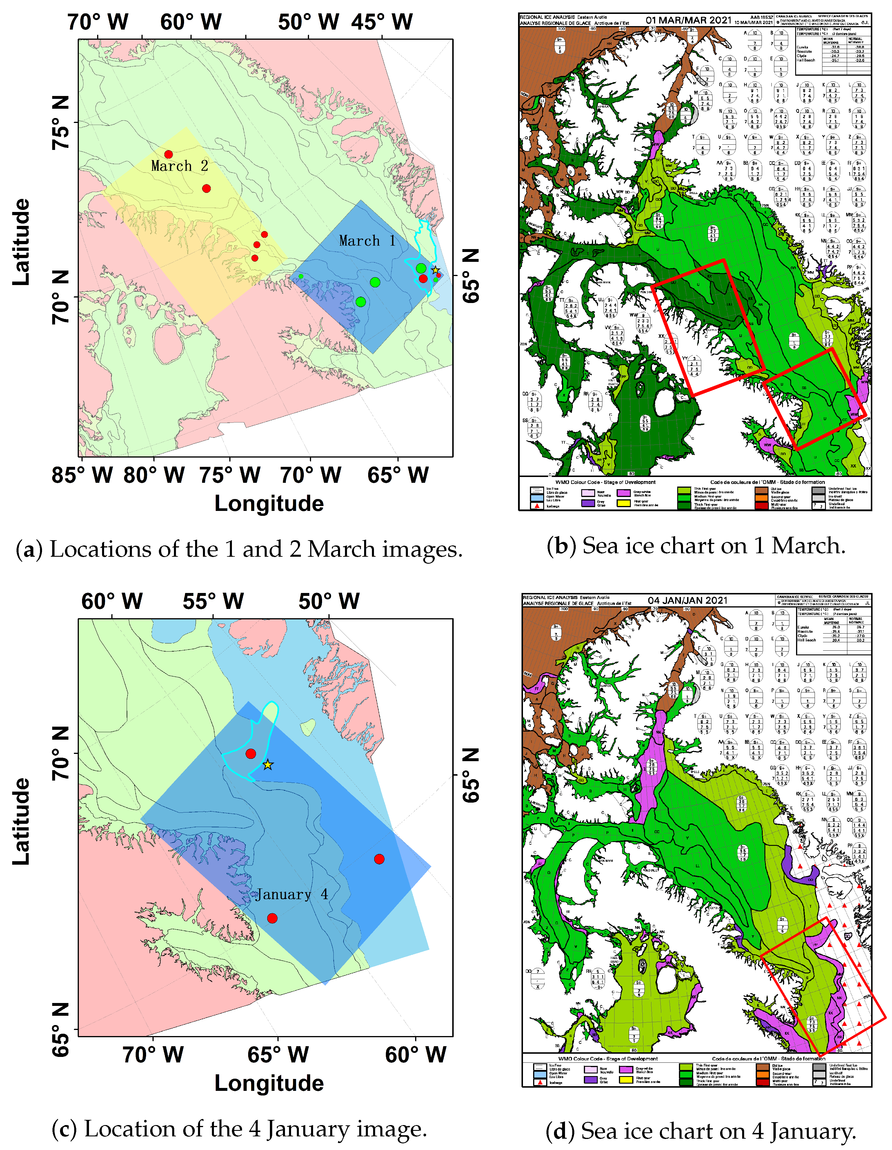
Three dual-polarized images, acquired on 4 January and 1 and 2 March 2021, were used and these are shown in Figure 1a,c. The information on the RCM images is summarized in Table 2. Sea ice classification can be affected by sea state conditions [37,43]. ERA5 [44] can provide global hourly ocean wave estimates based on reanalysis that combines physical models with observations from ground sensors and satellites, such as ERS-1, ERS-2 and Envisat. The stars in Figure 1a,c display the locations where the sea state information from ERA5 is used. At the acquisition time of the 1 March image around the Davis Strait, the significant wave height was 1.5 m, the period was 5.1 s and the direction was 173.3°. On 2 March, the significant wave height was 2.1 m, the period was 6.7 s and the direction was 176.6°. The yellow star on 4 January is close to the NI testing samples, where the significant wave height was 1.7 m, the period was 5.3 s and the direction was 241.3°. The red star in Figure 1c is located near the water testing samples, where the significant wave height was 1.5 m, the period was 5.7 s and the direction was 219.5°. According to the World Meteorological Organization (WMO) code [45], the sea states at the acquisition times of the three RCM images are moderate. Therefore, the training set and testing set were collected under similar sea-state conditions.
3.4. Training and Validation
In order to obtain reliable sea ice samples from the RCM data based on the digital sea ice chart to train a machine-learning-based classifier and evaluate its performance, a reasonable labeling strategy is required. Labeling is divided into two steps: automatic labeling and manual labeling. For the georeferenced RCM image, the longitude and latitude of each pixel are known, so the georeferenced coordinates are firstly converted into the Lambert Conic Conformal—Two Standard Parallels (2SP) projection format to match the projection mode of the digital sea ice chart. The sea ice chart polygon to which each pixel belongs can be determined. By reading the attribute of the corresponding polygon from the digital sea ice chart, each pixel’s egg code can be acquired. In this way, the initial automatic labeling can be realized. However, the sea ice chart cannot indicate specific sea ice information for each pixel, but rather for a polygon. In a polygon with a low sea ice concentration, the ice and water distribution is not specified. If the machine learning model is trained directly according to the automatically labeled pixels, a large number of pixels corresponding to water will be misclassified as ice. Therefore, manual labeling is required to generate more accurate training and testing samples.
In this study, only homogeneous areas completely covered by sea ice or water are selected for manual labeling. Next, inside these regions, only those parts that also look like ice in the RCM images were finally selected as training samples. Similar steps but with a concentration lower than 10% were used for the selection of water samples. Here, only three classification types are considered. Ice with a stage of development code of new ice to gray-white ice is labeled as NI, that with the code of first-year ice to old ice is labeled as old ice and first-year ice (OI/FYI, see Table 1). Considering that the polygons used for selecting the NI samples (illustrated in Figure 1a,c with blue borders) contain some other cover types, only the areas displayed as clearly bright in the pseudo-color images were used for the selection of the NI samples. The green and red dots indicate the locations for selecting the training and testing samples, respectively. These locations were chosen since each of them belongs to a large homogeneous area. Ice-free, open water and bergy water are labeled as water. Bergy water and open water both represent areas where the sea ice concentration is less than 10%. For this data set, the ice in bergy water was mostly glacier ice. Ten thousand training samples were selected from the 1 March image for each class.
In this study, two testing sets were adopted. For the first testing set, ten-thousand OI/FYI samples were obtained from the 2 March image, whereas ten-thousand NI and ten-thousand water testing samples were obtained from the 1 March image and 10 km away from the training samples, since the 2 March one rarely contained these two types. The region for selecting new-ice testing samples is highlighted with a blue border (see Figure 1a). The first testing set was from 1 March and 2 March, and both days shared the same sea ice chart. Little variation in sea ice condition was expected between these two days since the time difference was only one day. To further evaluate the generalization ability of the two classifiers through testing samples from different times and locations, the samples for the second testing set were only selected from the 4 January image and far away from the training samples in the 1 March image. For the second testing set, the OI/FYI and water testing samples were selected from the south portion of the 4 January image and more than 100 km away from the corresponding training samples. The NI samples of the second testing set were from the polygon outlined with a blue line in Figure 1c. Although some other regions in the 4 January image also contained NI, the highlighted area in Figure 1c was the farthest (more than 172 km) from the training samples. Because the NI samples of the training set only came from one polygon of the sea ice chart and the NI samples of the training set were different from that of the testing set in terms of both time and location, it could have been difficult for the classifiers to distinguish NI from other cover types. From another perspective, the NI classification results can also be utilized to compare the two models’ generalization ability.
The confusion matrix, kappa coefficient and overall accuracy were used to evaluate the classification performance based on those testing samples. Then, the total sea ice concentration statistics and the distribution percentages of different sea ice types in different areas were calculated and compared with the egg codes from the digital sea ice charts. The total concentration and distribution percentage can be determined by dividing the number of pixels of the corresponding ice type by the total number of pixels excluding land in a region. If an area contains land, the land is labeled via a land mask image. These land pixels are not involved in further analysis, including concentration and distribution calculations.
4. Methodology
4.1. Preprocessing
SAR data need to be preprocessed to enhance the data quality and meet different application requirements, for example, mitigating the noise from reflection and geometric distortion caused by terrain changes. Figure 2 displays the preprocessing steps for dual-polarized RCM images. The Sentinel Application Platform (SNAP) [46], developed by the European Space Agency (ESA), contains various free open source toolboxes for earth observation missions. In this paper, SNAP was employed to implement most preprocessing steps except destriping.
First, calibration was accomplished by converting two digital channels (HH, HV) of the RCM data into the backscattering coefficient in decibels, which indicates the target backscatter properties, according to [47]:
where B is the offset and A is the range dependent gain value that can be found in the RCM metadata file, D is the digital value for each pixel from the RCM tiff file.
For speckle filtering, the improved Lee sigma filter with a square window size of 7 by 7 was adopted [48]. This filter was modified from the Lee sigma filter by reducing the bias caused by asymmetric Rayleigh distribution, unfiltered black pixels and the smearing of strong targets [48]. In this study, a window with a side length of 7 was selected because it can achieve effective speckle filtering while maintaining more texture information [48].
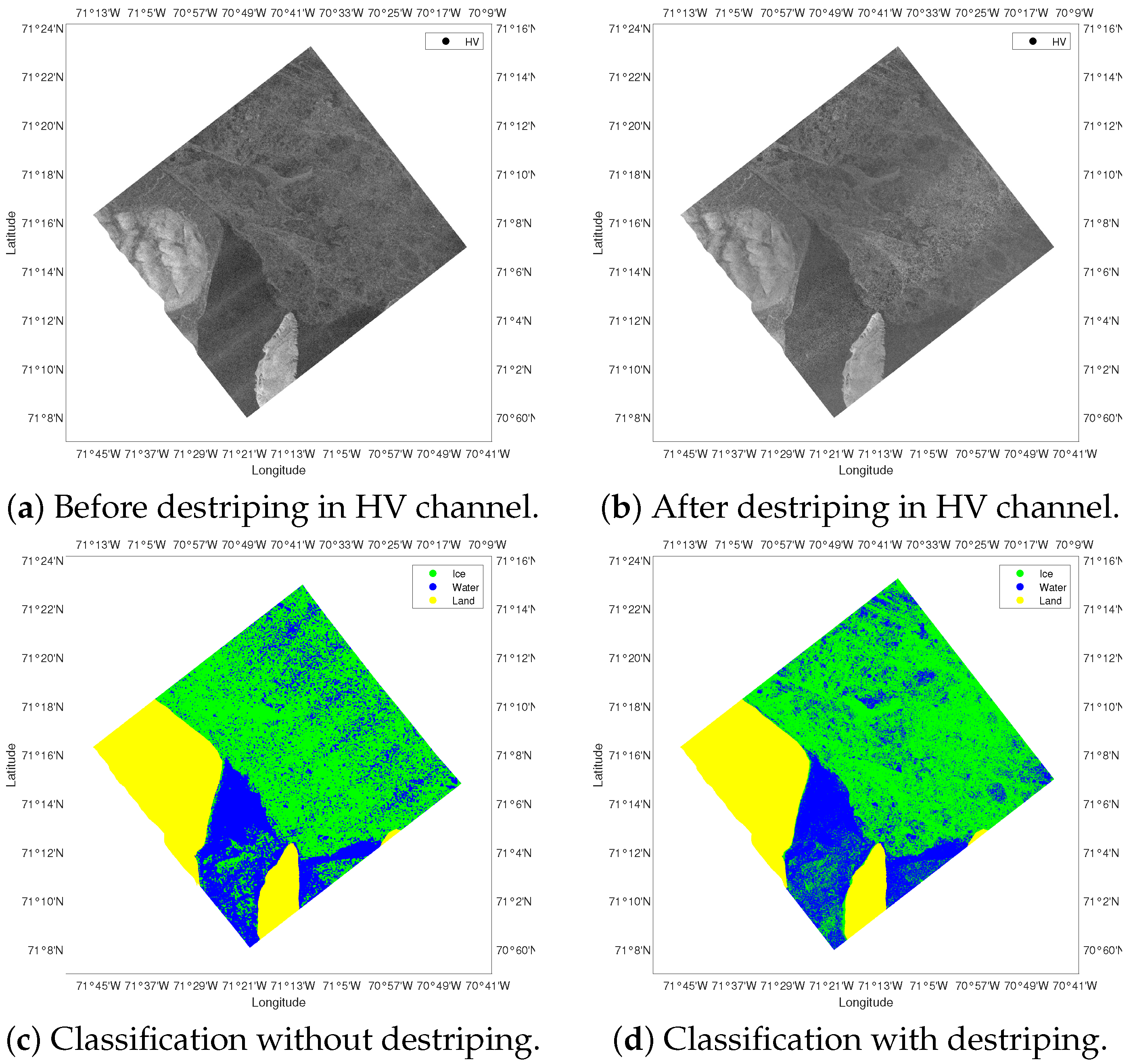
Thermal noise is an additive background energy, and it varies along both the range and azimuth axes and is exhibited as alternating extraordinarily bright or dark stripes in SAR images [49]. In addition to conventional SAR preprocessing steps, destriping is implemented as an extra step between speckle filtering and geocoding since thermal noise can significantly affect pixel-based sea ice classification. Note that the thermal noise in the HV channel is more evident than the HH channel in a linear polarized SAR image. Thus, destriping is only applied to the RCM HV channel here. Destriping is applied to each pixel of the RCM HV channel through subtracting an intensity offset and then dividing by a gain factor [50]. Figure 3a,b illustrate the images before and after applying destriping. As can be seen, the stripes of the HV channel are partially successfully removed after destriping. As shown in Figure 3c, ten-thousand samples for each class are used for training in this example. The blue pixels in the large green region are thermal noise and they are classified as water if destriping is not applied, but are classified correctly in Figure 3d.
Geocoding is implemented via range doppler terrain correction, which uses available orbit state vector information, the radar timing annotations, the slant-to-ground range conversion parameters in the metadata file with the reference Digital Elevation Model (DEM) data to derive the precise geolocation information [51]. The most commonly used DEM is SRTM, which only provides high-precision elevation data below 60 N. The study area is over 60 N, so Copernicus DEM GLO-30 was selected for geocoding because it provides global elevation data with a 30 m resolution. To realize automatic labeling as described in the last section, Lambert Conformal Conic 2SP was used for map projection, of which the projection parameters are consistent with the digital sea ice chart. Finally, land regions were masked out according to the DEM in order to avoid false labeling.
The value changes with the incidence angle for ice type, season, and radar frequency [23,52,53]. Most papers that consider incidence angle variability employ universal linear correction, which is based on an empirical linear relationship between mean sea ice backscattering and incidence angle value. Such a correction usually requires the sea ice type information to be known in advance. However, the ice types were known not for all the pixels in the preprocessing step. Thus, the incidence angle variability was ignored in this study.
4.2. Normalizer-Free ResNet
4.2.1. Normalizer-Free ResNet Architecture
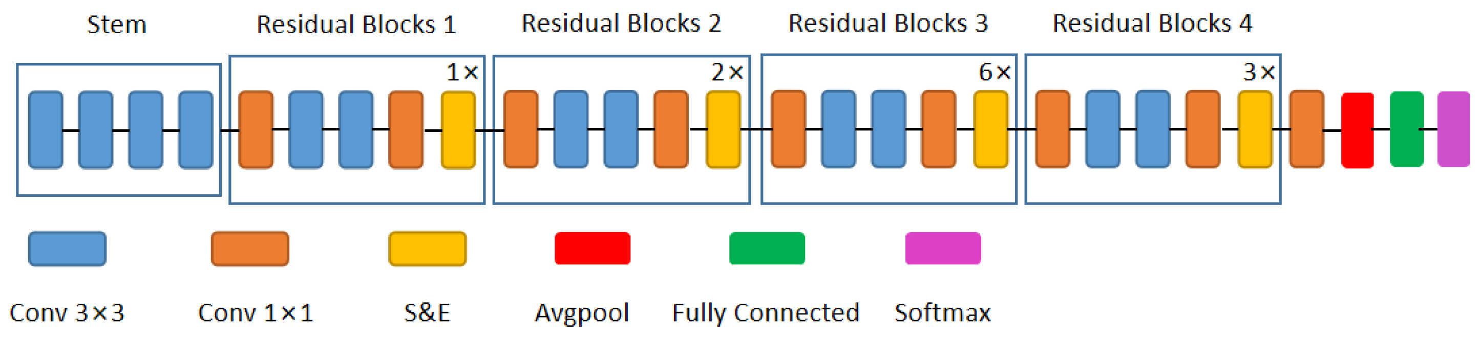
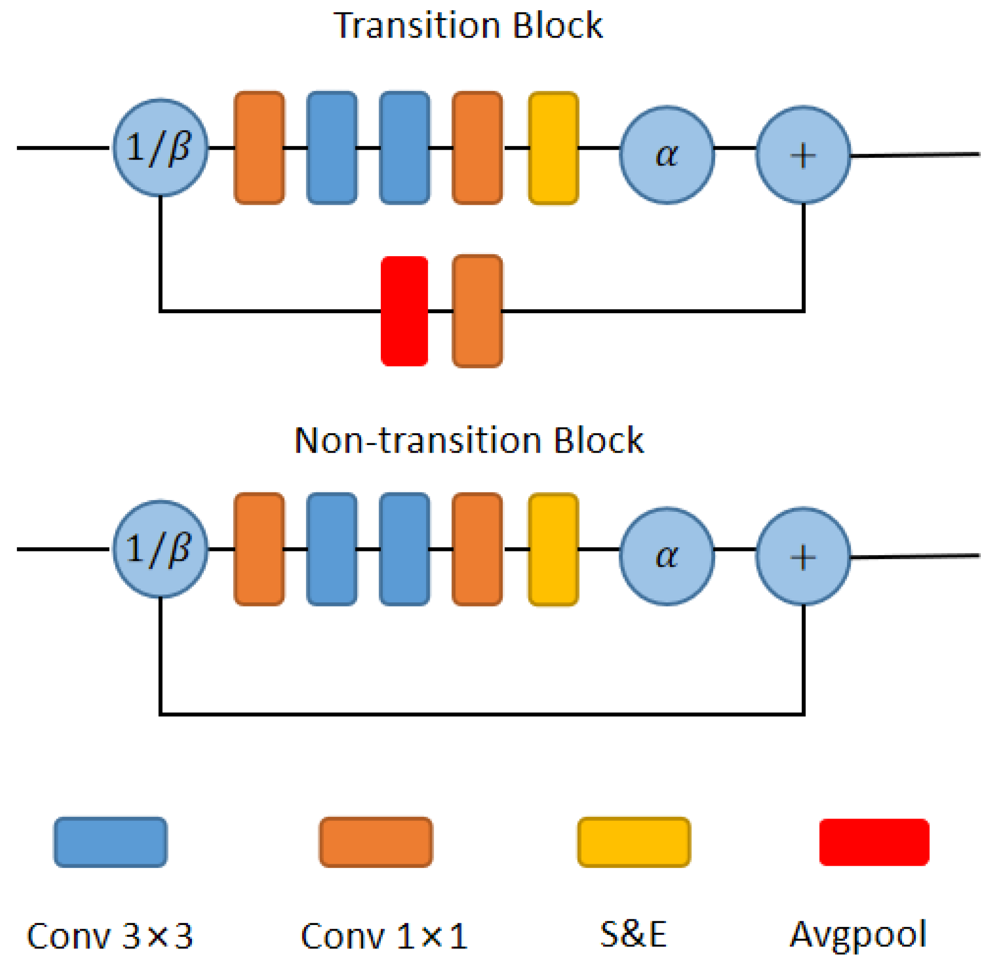
The NFNets were realized based on the SE-ResNeXt-D model with Gaussian error linear unit (GELU) activations here, and its structure is displayed in Figure 4. GELU activation layers were omitted between convolutional layers. The model starts with a stem, a set of plain convolutional layers without skip connections before the residual blocks. The stem comprises a 3 × 3 stride 2 convolution with 16 channels, two 3 × 3 stride 1 convolutions with 32 and 64 channels and a 3 × 3 stride 2 convolution with 128 channels. After the stem, the numbers of blocks for four “residual” stages are 1, 2, 6 and 3, respectively. In order to train deep ResNets without normalization, NFNet uses two scalers ( and , see Figure 5) to suppress the scale of the activations. The residual stages begin with a transition block, followed by standard non-transition blocks. The difference between transition and non-transition blocks is that transition blocks downsample with a 2 × 2 average pooling layer on the skip path and change the output channel count via a 1 × 1 shortcut convolutional layer. After these residual blocks, a 1 × 1 expansion convolutional layer is applied to double the channel count; then, global average pooling is adopted. The final layer is a fully connected classifier layer. The original fully connected layer outputs a 1000-way class vector. In our study, we replace the final layer with a layer that outputs a three-way class vector to match the sea ice types. At last, the fully connected layer outputs are softmaxed in order to obtain normalized class probabilities. All convolutions employ scaled weight standardization, whereas the squeeze-and-excitation layers and fully connected layers do not adopt it. The configuration of each layer is specified in Table 3.
4.2.2. Adaptive Gradient Clipping
Batch normalization (BN) is widely used in deep learning to rearrange the data distribution, making the activation function more sensitive to training data. However, BN also has some disadvantages. First, it is an expensive computational operation, which incurs memory overhead and increases the time of gradient evaluation [31]. Second, it introduces inconsistencies between the behaviors of the model during training and at inference time due to the change in the data distribution, resulting in additional hidden hyper-parameters that have to be tuned [31]. Third, it is difficult to replicate batch-normalized networks precisely on different hardware. Different hardware may be used to train different batches of data at the same stage since some GPUs with low RAM cannot be used to train a model with a very high batch size [31].
Adaptive gradient clipping (AGC) is applied in the Normalizer-Free ResNet (NFNet) to train ResNets without batch normalization. In the AGC algorithm, the ith row of the gradient of the l-th layer is clipped as [31]:
where is the clipping threshold, and , with default ; denotes the Frobenius norm.
4.2.3. Preprocessing of the Inputs
HH, HV and the cross-polarization ratio were extracted from the RCM images as inputs. In this study, the cross-polarization ratio was defined as and was used as an input channel for the NFNet classification, since it was found to be able to improve the discrimination between open water and ice types [2]. The patch size was set to 7 × 7 to compare with the RF method (the window size of GLCM features for RF is 7 × 7). Since the inputs fed into the NFNet are supposed to be fixed in size, all the sampled sub-regions were first resized using bilinear interpolation. In this study, NFNet-F0 was adopted here and its input size for training was 192 × 192 × 3, and 256 × 256 × 3 for testing. Then, the resized inputs were normalized using mean = [0.485, 0.456, 0.406], and std = [0.229, 0.224, 0.225] for three input channels, respectively [31].
4.2.4. Training Strategy
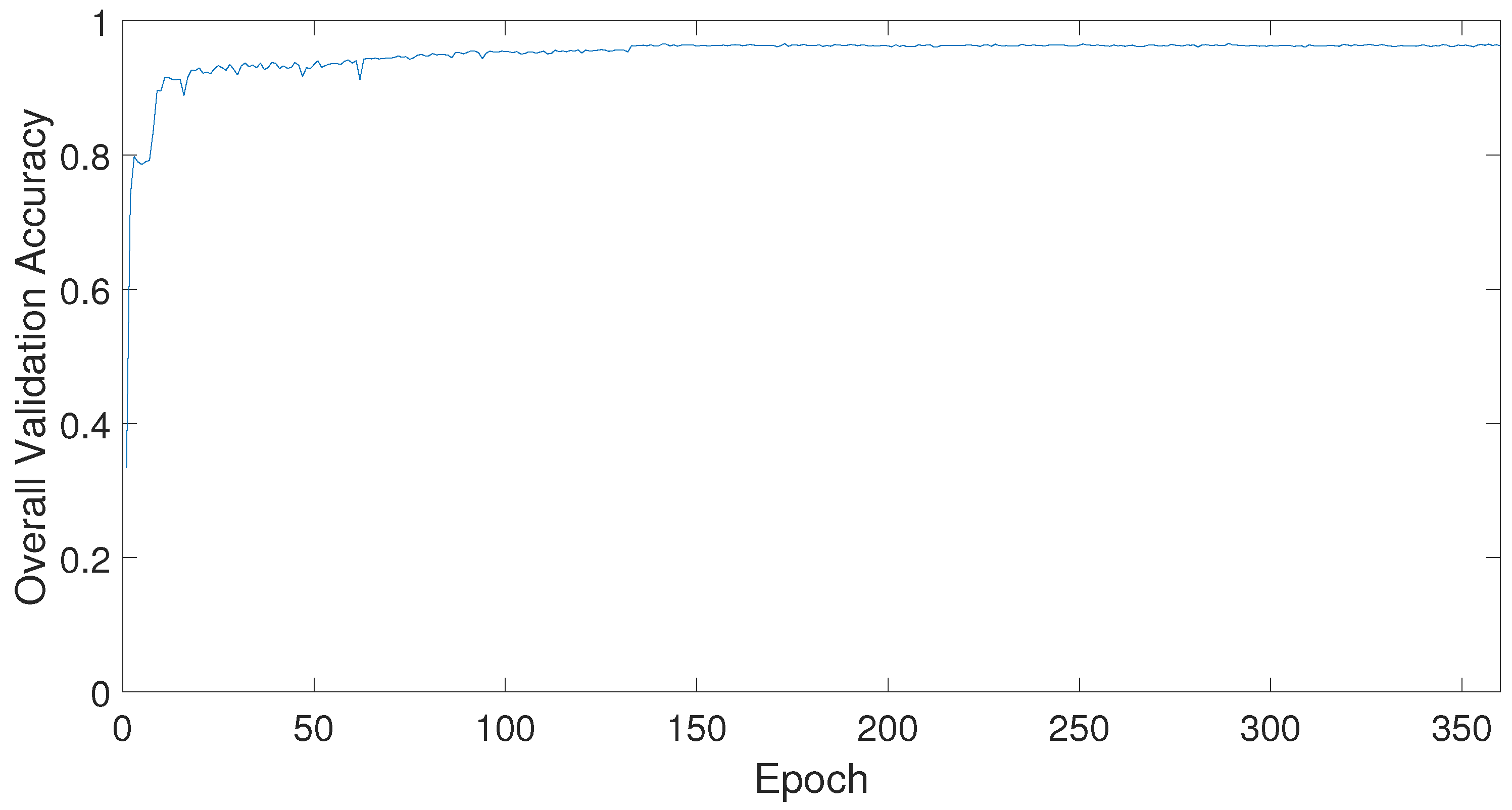
The training strategy of the NFNet-F0 was basically the same as that in [31]. Softmax cross-entropy loss was used with label smoothing of 0.1. Stochastic gradient descent was applied with Nesterov’s momentum coefficient of 0.9 and a weight decay coefficient of 0.00002. The learning rate warmed up from 0 to its maximal value of 0.05 over the first five epochs (iterations). After the warmup, the learning rate was cosine-annealed to zero. AGC was set with for every parameter except the fully connected layer. An exponential moving average was implemented with a decay rate of 0.99999 and followed a warmup schedule where the decay was equal to , where t was the number of iterations. The batch size was set as 128. For the training process, 70% of samples were used to train the model, and 30% of samples were used to evaluate the model’s generalization ability. Three hundred and sixty epochs were executed to train the model. Figure 6 shows the validation accuracy changes with epochs during the training process. After about 130 epochs, the validation accuracy of the model tended to be stable. The model with the best validation accuracy was obtained for subsequent classifications.
4.3. Random Forest
Various machine learning algorithms have been applied for sea ice sensing in the past decade, such as the support vector machine (SVM) [54], convolutional neural network (CNN) [55], and long short-term memory (LSTM) [56] methods. In this study, random forest (RF) was adopted as the basic classifier to compare with NFNet. The RF method was the same as that of our previous work on sea ice detection using RCM dual-polarized data [57]. RF is an ensemble machine-learning technique that creates a group of decision trees (DTs) as weak learners [58]. The majority of votes decide the classification result from these decision trees. DTs are trained by means of a bagging strategy that generates multiple bootstrapped data sets from the original training data. Because of the use of bagging and ensemble strategies, the RF classifier is characterized by low variance and low bias, which means it is robust and less sensitive to the quality of the training data [58]. Two levels of RF classification were applied in this study. Ice and water were classified for the 1st level, then the identified ice pixels were classified as NI or OI/FYI at the 2nd level.
HH, HV, the cross-polarization ratio and the gray-level co-occurrence matrix (GLCM) features of the RCM dual-polarized GRD images were used for sea ice detection and classification. GLCM represents the frequency that a pixel pair in a specific direction appears in a grayscale image. First, the grayscale image was normalized to n levels. Then, the number of times every possible pair (for example, 0,1) appeared in a particular direction was counted and filled into the corresponding matrix for this direction. For example, in a horizontal GLCM indicates that the pair () in the horizontal direction appears m times, and m is located at the ith row and jth column in the matrix. After that, the mean, variance, correlation, homogeneity, contrast, dissimilarity, entropy, angular second moment and maximum probability can be calculated according to the GLCM matrix. These features can be used as texture features for further analysis. According to [59], 64 levels and 4 (0, 45, 90, 135) orientations were the recommended GLCM parameters for sea ice detection in SAR images. For this study, a displacement of 1 and window of size were selected. Such a window size was selected in order to be consistent with the speckle-filtering window. The authors of [60] investigated the nine GLCM features and found that mean and variance were effective for both HH and HV channels. In this study, a mean displacement and mean orientation (MDMO) strategy for GLCM was applied. In other words, the average values of the GLCM mean and variance in four orientations of one channel were extracted separately. Finally, four features (the GLCM mean of HH, GLCM variance of HH, GLCM mean of HV and GLCM variance of HV) were obtained.
Ten-thousand samples from 1 March were labeled for each class. The number of trees, maximum tree depth, maximum features, minimum samples-split and minimum samples-leaf were tuned based on five-fold cross-validation. After cross-validation, the parameters for the two-level RF model were set as shown in Table 4.
5. Experiment Result
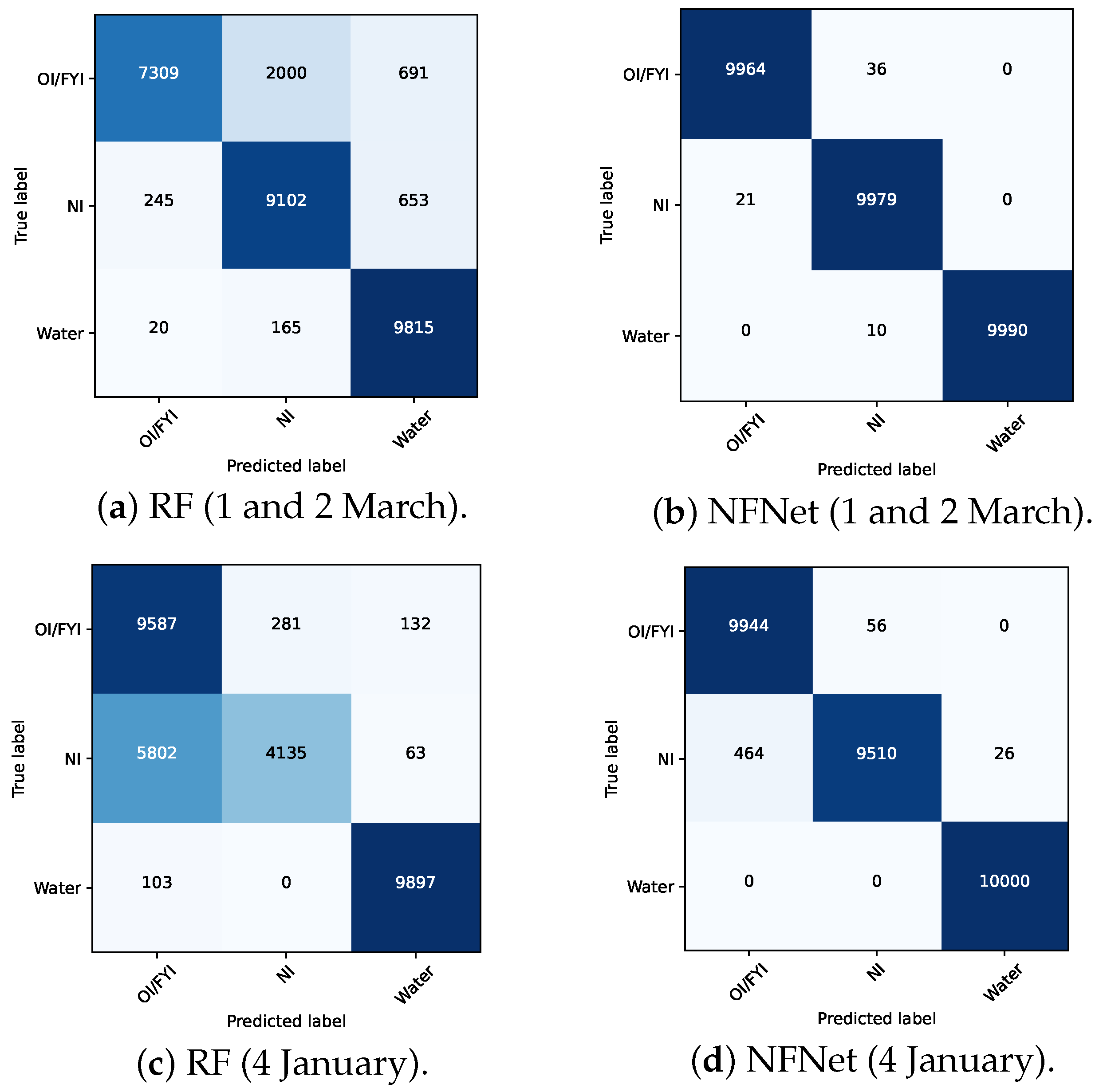
Figure 7, Figure 8 and Figure 9 illustrate the analysis results for 1 March, March 2 and 4 January, respectively. The green rectangles in Figure 7a were used for selecting the training samples for OI/FYI. The red and white rectangles indicate the areas used for selecting the training and testing samples of NI and water, respectively, and their testing samples were located far away from corresponding training samples, as mentioned in Section 3.4. The green rectangles presented in Figure 8a were used for extracting the OI/FYI samples for the first testing set. Ten-thousand samples for each class of the second testing set were obtained from the rectangles displayed in Figure 9a. Compared to the training samples, the corresponding second testing samples were taken from a different time (4 January) and different regions. All the testing samples for the two techniques were the same. The RF method’s overall accuracy and the kappa coefficient of the first testing set were 87.42% and 0.8113, respectively. For the NFNet classification, the first testing set’s overall accuracy was 99.78%, and the corresponding kappa coefficient was 0.9967. As for the second testing set, the RF’s overall accuracy and kappa coefficient were 78.73% and 0.6895, whereas NFNet’s overall accuracy and kappa coefficient were 98.18% and 0.9727. Although different data sets and cover types were used, the overall accuracies of RF (87.42% and 78.73%) and NFNet (99.78% and 98.18%) in this study were close to that of RF (87%) in [23] and VGG-16 (99.89%) in [28]. The corresponding confusion matrices are displayed in Figure 10. For the first testing set (see Figure 10a,b), no ice samples were misclassified by the NFNet as water. For the RF model, the classification accuracy for water was only 87.96%, which means that more ice samples were misclassified as water. Moreover, the recall of OI/FYI was 73.09%. For the two-level RF model, OI/FYI was classified at the second level, distinguishing OI/FYI and NI from ice samples. The poor recall for OI/FYI indicates that many OI/FYI samples were misclassified as NI. Figure 10c,d illustrate the confusion matrices of the two models for the second testing set. It can be seen that the accuracy of the NFNet for NI only dropped slightly. The 100% accuracy for water displayed by the NFNet may be because these water samples were very far from the main ice area. Only 41.35% of the NI samples from the second testing were correctly classified for the RF method, and more than half of the NI samples were misclassified as OI/FYI.
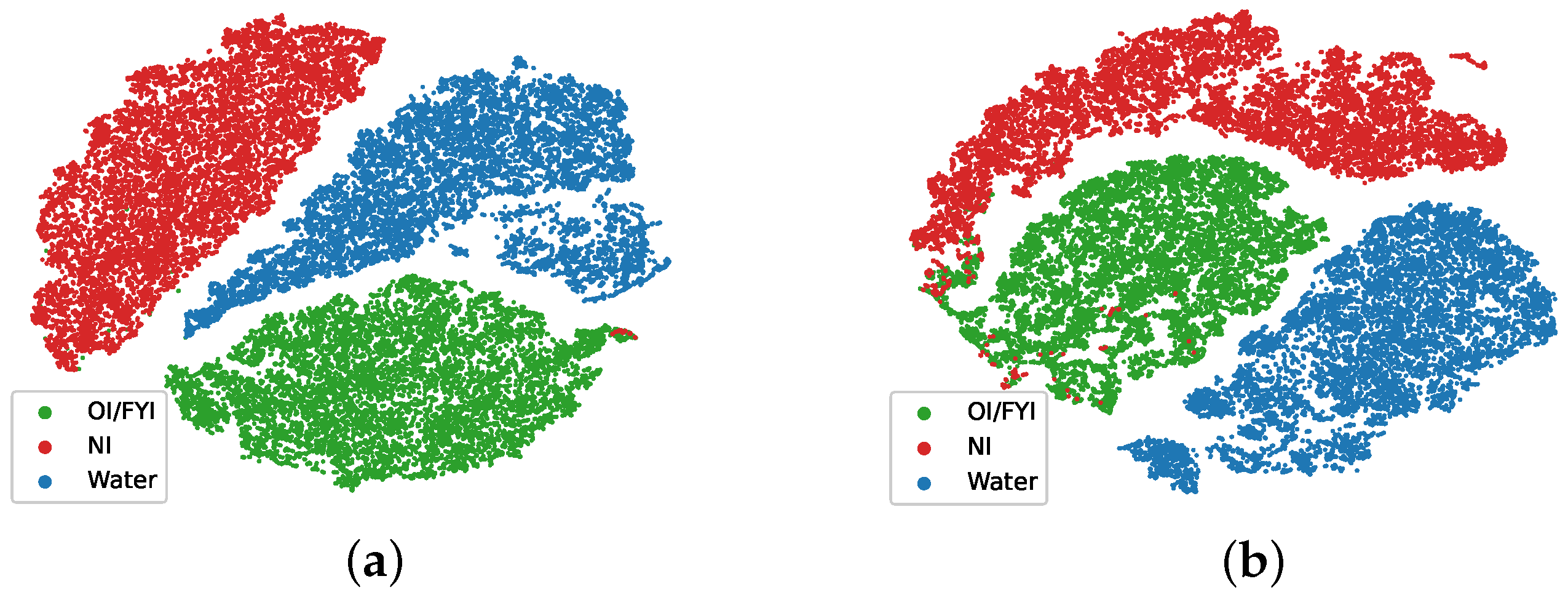
Figure 11 illustrates the t-SNE images of the second last layer of the NFNet, which illustrates the ability of the model to distinguish between sea ice and water. Thirty-thousand testing samples were applied as inputs to display each t-SNE diagram. The features from the NFNet were perfectly clustered. However, the feature clusters of OI/FYI and NI showed some degree of confusion.
Table 5, Table 6 and Table 7 show comparisons of the sea ice chart data, the RF and NFNet results. In these tables, the “area ratio” represents the ratio of the area of a polygon (which may be incomplete) in an RCM image to that of the corresponding complete polygon in the sea ice chart. A higher area ratio for a polygon means that the data for this area shown in the RCM image are more representative than those of the complete polygon.
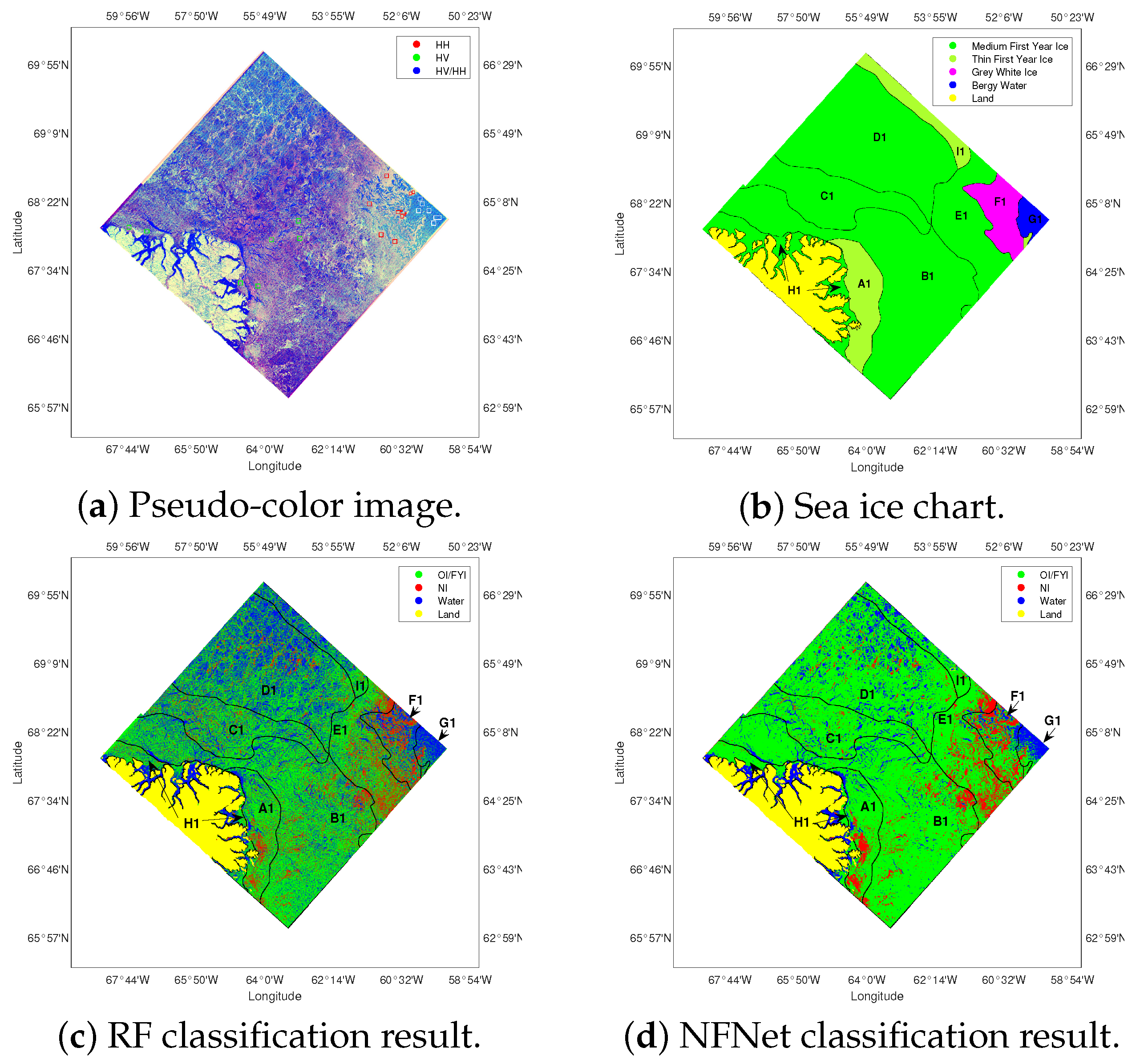
Figure 7 demonstrates the classification results of the full image from 1 March. As mentioned earlier, the training samples for the two-level RF classification model and the NFNet model were selected from this image. Figure 7d,e depict the RF and NFNet classification results. Although only samples from region G1 were labeled as water, both classification results show that all the dark blue regions in the pseudo-color images were identified as water. In general, more regions were classified as water by RF than NFNet. Both classifiers detected NI at approximately the same locations. Although more pixels were classified as NI by the RF model, except in region F1, for which the NI concentrations estimated using the two models were very close, with a difference of only 0.5% (see Table 5). In the digital sea ice chart, no NI was reported in regions B1, C1, D1, G1, H1 or I1. However, both methods detected less than 10% NI in these regions. According to the notation principles of sea ice chart [42], any ice type with a concentration less than 10% would not be reported; therefore, the NI estimation results of these regions are reasonable. Meanwhile, the NI concentrations of regions A1, E1 and F1 derived using the two models were higher than 10%, but the sea ice chart reports very high NI concentrations in regions A1 (40%) and F1 (60%) and no NI in region E1. Because the training samples of NI were only selected from the subarea with a uniform ice distribution in region F1, but NI includes many types (rind, nilas, gray ice, gray-white ice, etc.) and forms (pancake, ice cake, ice floe, etc.) that may show different scattering characteristics [42], the training data may not represent all the types of NI in the regions, which leads to the estimation difference in these areas. Although the sea ice chart reports no NI in E1, both RF and NFNet detected NI at similar locations, and their concentration values were also very close. The area ratio of E1 was only 41%, indicated that perhaps there was very little NI in the portion that belonged to the same polygon E1 but was not covered by the RCM image. Moreover, considering that E1 is adjacent to F1, it is reasonable that NI exists in E1. Thus, the results of NFNet and RF may be more reliable than the weekly sea ice chart for region E1. As for the total concentration, the results of RF and NFNet were in agreement with the sea ice chart data for most of the regions, with the former showing a better agreement. In particular, the RF-estimated total ice concentrations of D1 and I1 were 61% and 59.2%, respectively, which were not consistent with the sea ice chart (90%+ for both regions, see Table 5. On the contrary, NFNet’s results were 85.3% and 80.9% for these two regions. Considering that no training data came from D1 and I1, this difference proves that the generalization ability of NFNet was better than that of RF. In addition, the sea ice concentrations of G1 estimated by both classifiers were higher than 10%, although the sea ice chart displays a concentration less than 10%. However, the area ratio of G1 was only 0.1%, which means that only the edge of the polygon G1 was covered by the RCM image from 1 March and the value is very unrepresentative. Therefore, the deviation of the two classifiers in G1 is understandable. It can also be observed that the classification results for the regions near the coast are similar for both classifiers. Based on the above analysis, it can be inferred that the NFNet method can produce more reasonable sea ice estimation results than the RF method.
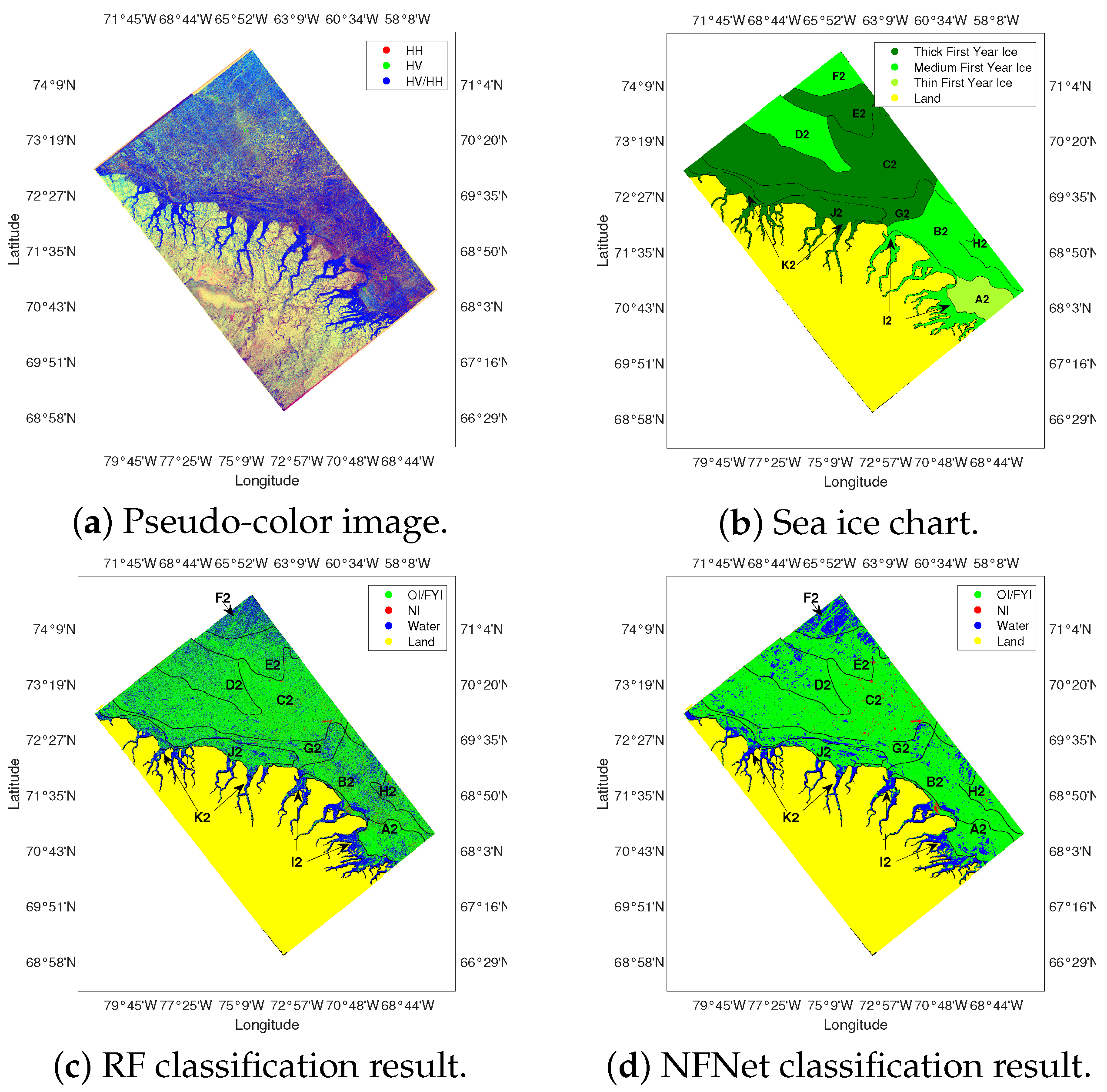
The classification results from the image acquired on March 2 are displayed in Figure 8d,e. It should be highlighted that no samples from the March 2 image were used for training the classification models. Similarly to the 1 March image results, both models provided good classification results in general, and more water regions were identified by the RF model than the NFNet. The NI percentages in both results were also very low, which was in agreement with the digital sea ice chart. The total sea ice concentration estimation results of the NFNet obtained from A2, B2, C2, D2, E2 and G2 were consistent with that of the sea ice chart, except for F2 (see Table 6). Considering that F2 had the lowest area ratio (4.4%) in the March 2 image, only part of this polygon was analyzed and the results may not represent the sea ice condition of the majority of the polygon, so this deviation is reasonable. It can be seen in Figure 7 and Figure 8 that H1, I2, J2 and K2 are next to the coast. The sea ice chart reported that those regions were occupied by fast ice, which was “fastened” to the coastline and can extend from a few meters or several hundred kilometers from the coast [42]. For fast ice regions, there were some gaps between the estimation results and the sea ice chart data. Although J2’s area ratio was close to 100% and the corresponding sea ice chart data indicated that this area was covered by consolidated ice (100% concentration), the pseudo-color image Figure 8a exhibits many dark blue strips (i.e., water) in this area. Therefore, at least on March 2, the sea ice concentration in J2 should not be 100%. Furthermore, the time resolution of the sea ice chart adopted here was one week; therefore, the estimations of NFNet and RF are more reasonable. The difference between manually drawn ice charts and automatic ice charts is discussed in [61]. Manually drawn ice charts are affected by the education and experience of the ice analysts. Even using the same data source, different ice experts may produce different sea ice charts. Moreover, manually drawn ice charts show rough boundaries and relatively poor detail, whereas automatic ice charts can help to interpret image information more rigorously and distinguish more segments [61]. In the traditional manual production of weekly regional ice charts, their main data sources are satellite images, as well as corresponding daily ice analysis charts [42]. The ice charts are manually drawn directly by ice experts using geographic information systems (GIS) software [42]. However, it is time-consuming for ice experts to analyze many satellite images, and pixel-level classification is impossible [61]. In contrast, once the machine-learning-based classifiers are trained properly using a data set with a sufficient amount and diversity, near real-time classified results can be generated, and pixel-level classification can be achieved. In this study, the classified results can also be used to estimate the concentration in a region with a specific value rather than a rough concentration code.
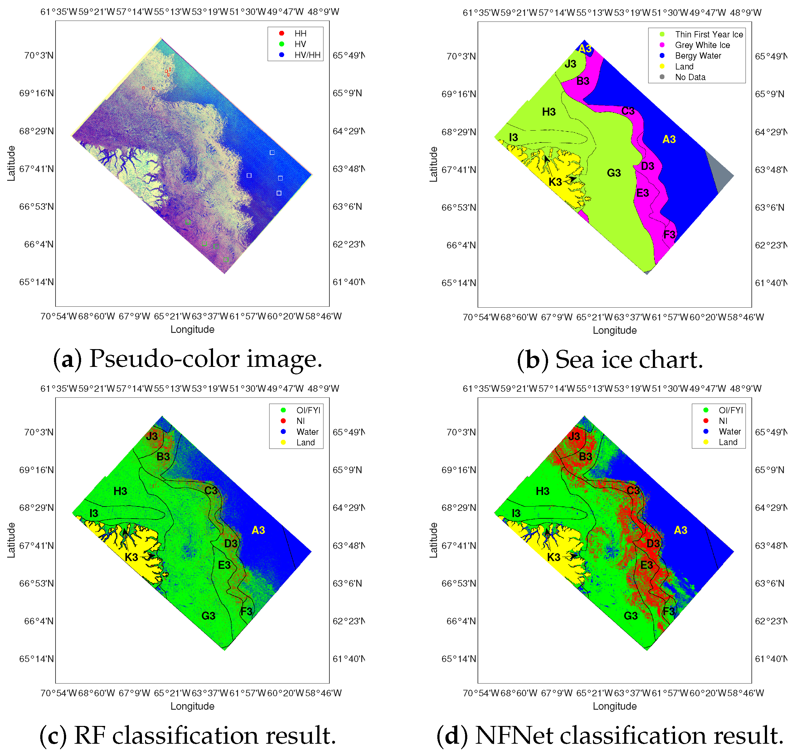
In order to demonstrate the robustness of the method in terms of location and time, another image (see Figure 9a) that was collected from different areas and times (4 January) was used. The classification results from this image are displayed in Figure 9d,e. Both models provided good classification results for OI/FYI and water. However, the RF model identified fewer NI regions than the NFNet. The NI percentages in both results were lower than those of the sea ice chart (see results of B3, D3, E3, F3 and G3, which are highlighted in bold in Table 7), but the NI concentrations estimated by NFNet were closer to those of the sea ice chart. In other words, NFNet provides better generalization ability for NI than the RF method. For C3 and J3, the NI concentration obtained by RF was close to the corresponding reports of the sea ice chart, whereas the NI concentration determined by RF was much higher. Considering the relatively poor performance of the RF classifier for these regions and the fact that the pseudo-color image (Figure 9a) also shows that C3 and J3 regions are uniformly bright white (i.e., covered by new ice), the NI classification by NFNet should be more reliable. The total concentration differences of A3 and K3 are also due to the presence of landfast ice and glacier ice, as discussed above. For F3, the total concentrations estimated by the two classifiers were both significantly higher than the sea ice chart results. The pseudo-color image (Figure 9a) shows that only a tiny proportion of F3 is blue (i.e., covered by water), so the total concentration of F3 should be higher than 50%, at least for 4 January.
6. Discussion
According to the experimental results, the high accuracy and kappa coefficient show the superior capacity of the NFNet model over the RF model. Confusion matrices indicate that the RF model underestimated the total concentration and significantly underestimated the NI concentration due to the time difference. The challenge of classifying the new ice types is also demonstrated in previous works [17,19,23]. However, the NFNet model showed more generalization ability for classifying NI than the RF model. Although our training dataset was unbalanced and limited, considering the classification performance of the deep CNN after obtaining enough diverse data, the NFNet also shows the potential to classify NI more accurately than conventional machine learning techniques. The t-SNE diagram generated using the second testing set shows that more samples of NI were interlaced with the OI/FYI samples, which means that the NI classification accuracy of the NFNet may differ slightly due to the difference in the time and location of the samples. For the classification results of the whole images, both models showed an appropriate ability to distinguish between water and ice. By comparing the sea ice concentrations calculated based on the classification results with the concentrations obtained from sea ice charts, the NFNet results were not only better than those of RF but were also more accurate than the sea ice charts.
7. Conclusions
This paper presents the first case study of a sea ice classification application using actual RCM dual-polarized data with a state-of-the-art technique (NFNet). Destriping was considered to mitigate the thermal noise in the HV channel in addition to conventional SAR preprocessing steps. HH, HV and the cross polarization ratio were extracted from three RCM images, collected from the Eastern Arctic for the NFNet sea ice classifier. The classification results were validated using digital sea ice charts and testing samples that were different from the training samples in both space and time. A two-level RF classifier was applied as a conventional machine learning method in comparison with the NFNet method. The experimental results showed that a high accuracy of sea ice classification was achieved using dual-polarized RCM data. Good classification results proved the superiority of NFNet-based sea ice classification over the conventional RF technique. Due to the learning algorithm difference between NFNet and RF, the former achieved higher overall sea ice classification accuracies (99.78% and 98.18% for two testing sets) compared to RF (87.42% and 78.73%), indicating the superiority of NFNet over the conventional RF technique based on the RCM data used here. Whether or not the same conclusion can be drawn from other SAR data requires further testing. In this paper, the ERA5 sea-state information showed that the training set and the testing set were collected under similar sea-state conditions, so the effect of sea state was not comprehensively analyzed due to limited data, but this remains as a future task. It should be noted that other factors that affect the classification quality, such as wind speed, season, incident angle and patch size for the NFNet model, were not considered. In the future, the internal and external factors affecting sea ice classifications will be investigated. Moreover, actual HCP data will be used for sea ice classifications and compared with the performance of RCM dual-polarization mode.
Author Contributions
All authors made substantial contributions to the conception and the design of the study. W.H. and H.L. performed the experiments, analyzed the data and wrote the paper. Formal analysis, H.L., W.H. and M.M.; Funding acquisition, W.H.; Methodology, H.L., W.H. and M.M.; Writing—original draft, H.L.; Writing—review and editing, W.H. and M.M. All authors reviewed and commented on the manuscript. All authors have read and agreed to the published version of the manuscript.
Funding
This research was undertaken thanks in part to funding from the Canada First Research Excellence Fund, through the Ocean Frontier Institute. This work was also supported by the Natural Sciences and Engineering Research Council of Canada (NSERC) under Grants [NSERC RGPIN-2017-04508] and [NSERC RGPAS-2017-507962] to W. Huang.
Institutional Review Board Statement
Not applicable.
Informed Consent Statement
Not applicable.
Data Availability Statement
Restrictions apply to the availability of the RADARSAT Constellation Mission (RCM) data used in this study. Data were obtained from Canadian Space Agency (CSA) and are available from the Earth Observation Data Management System (EODMS) with the permission of CSA.
Acknowledgments
The authors thank the Canadian Space Agency (CSA) for providing the RADARSAT Constellation Mission (RCM) data (RADARSAT Constellation Mission Imagery © Government of Canada (2021). RADARSAT is an official mark of the Canadian Space Agency.
Conflicts of Interest
The authors declare no conflict of interest.
References
- Dierking, W. Sea ice monitoring by synthetic aperture radar. Oceanography 2013, 26, 100–111. [Google Scholar] [CrossRef]
- Zakhvatkina, N.; Smirnov, V.; Bychkova, I. Satellite SAR data-based sea ice classification: An overview. Geosciences 2019, 9, 152. [Google Scholar] [CrossRef] [Green Version]
- Yan, Q.; Huang, W. Spaceborne GNSS-R sea ice detection using delay-doppler maps: First results from the U.K. TechDemoSat-1 mission. IEEE J. Sel. Top. Appl. Earth Obs. Remote Sens. 2016, 9, 4795–4801. [Google Scholar] [CrossRef]
- Lu, J.; Heygster, G.; Spreen, G. Atmospheric correction of sea ice concentration retrieval for 89 GHz AMSR-E observations. IEEE J. Sel. Top. Appl. Earth Observ. Remote Sens. 2018, 11, 1442–1457. [Google Scholar] [CrossRef]
- Lindell, D.B.; Long, D.G. Multiyear Arctic sea ice classification using OSCAT and QuikSCAT. IEEE Trans. Geosci. Remote Sens. 2016, 54, 167–175. [Google Scholar] [CrossRef]
- Alexander, D.; Fraser, R.A.M.; Michael, K.J. Generation of high-resolution East Antarctic landfast sea-ice maps from cloud-free MODIS satellite composite imagery. Remote Sens. Environ. 2010, 114, 2888–2896. [Google Scholar]
- Yan, Q.; Huang, W. Sea ice remote sensing using GNSS-R: A review. Remote Sens. 2019, 11, 2565. [Google Scholar] [CrossRef] [Green Version]
- Thompson, A.A. Overview of the RADARSAT Constellation Mission. Can. J. Remote Sens. 2015, 41, 401–407. [Google Scholar] [CrossRef]
- Raney, R.K.; Brisco, B.; Dabboor, M.; Mahdianpari, M. RADARSAT Constellation Mission’s operational polarimetric modes: A user-driven radar architecture. Can. J. Remote Sens. 2021, 47, 1–16. [Google Scholar] [CrossRef]
- Brisco, B.; Mahdianpari, M.; Mohammadimanesh, F. Hybrid compact polarimetric SAR for environmental monitoring with the RADARSAT Constellation Mission. Remote Sens. 2020, 12, 3283. [Google Scholar] [CrossRef]
- Huntley, D.; Rotheram-Clarke, D.; Pon, A.; Tomaszewicz, A.; Leighton, J.; Cocking, R.; Joseph, J. Benchmarked RADARSAT-2, SENTINEL-1 and RADARSAT Constellation Mission change-detection monitoring at North Slide, Thompson River Valley, British Columbia: Ensuring a landslide-resilient national railway network. Can. J. Remote Sens. 2021, 47, 635–656. [Google Scholar] [CrossRef]
- Choe, B.H.; Blais-Stevens, A.; Samsonov, S.; Dudley, J. Sentinel-1 and RADARSAT Constellation Mission InSAR assessment of slope movements in the Southern Interior of British Columbia, Canada. Remote Sens. 2021, 13, 3999. [Google Scholar] [CrossRef]
- Howell, S.E.L.; Brady, M.; Komarov, A.S. Large-scale sea ice motion from Sentinel-1 and the RADARSAT Constellation Mission. Cryosphere Discuss. 2021, 2021, 1–20. [Google Scholar] [CrossRef]
- De Roda Husman, S. Polarimetric SAR Signals of River Ice Breakup. Master’s Thesis, Civil Engineering and Geosciences, Delft University of Technology, Delft, The Netherlands, 2020. [Google Scholar]
- Komarov, A.S.; Buehner, M. Sea ice concentration from the RADARSAT Constellation Mission for numerical sea ice prediction. In Proceedings of the IEEE 19th International Symposium on Antenna Technology and Applied Electromagnetics, Winnipeg, MB, Canada, 8–11 August 2021; pp. 1–2. [Google Scholar]
- Kruk, R.; Fuller, M.C.; Komarov, A.S.; Isleifson, D.; Jeffrey, I. Proof of concept for sea ice stage of development classification using deep learning. Remote Sens. 2020, 12, 2486. [Google Scholar] [CrossRef]
- Dabboor, M.; Geldsetzer, T. Towards sea ice classification using simulated RADARSAT Constellation Mission compact polarimetric SAR imagery. Remote Sens. Environ. 2014, 140, 189–195. [Google Scholar] [CrossRef]
- Ren, P.; Yu, Z.Q.; Dong, G.S.; Wang, G.X.; Wei, K. Sea ice classification with first-order logic refined sliding bagging. J. Coast. Res. 2019, 90, 129–134. [Google Scholar] [CrossRef]
- Zhang, L.; Liu, H.; Gu, X.; Guo, H.; Chen, J.; Liu, G. Sea ice classification using TerraSAR-X ScanSAR data with removal of scalloping and interscan banding. IEEE J. Sel. Top. Appl. Earth Obs. Remote Sens. 2019, 12, 589–598. [Google Scholar] [CrossRef]
- Yu, Z.; Wang, T.; Zhang, X.; Zhang, J.; Ren, P. Locality preserving fusion of multi-source images for sea-ice classification. Acta Oceanol. Sin. 2019, 38, 129–136. [Google Scholar] [CrossRef]
- Han, H.; Im, J.; Kim, M.; Sim, S.; Kim, J.; Kim, D.j.; Kang, S.H. Retrieval of melt ponds on Arctic multiyear sea ice in summer from TerraSAR-X dual-polarization data using machine learning approaches: A case study in the Chukchi Sea with mid-incidence angle data. Remote Sens. 2016, 8, 57. [Google Scholar] [CrossRef] [Green Version]
- Lohse, J.; Doulgeris, A.; Dierking, W.; Lohse, J.; Doulgeris, A.P.; Dierking, W. An optimal decision-tree design strategy and its application to sea ice classification from SAR imagery. Remote Sens. 2019, 11, 1574. [Google Scholar] [CrossRef] [Green Version]
- Park, J.W.; Korosov, A.A.; Babiker, M.; Won, J.S.; Hansen, M.W.; Kim, H.C. Classification of sea ice types in Sentinel-1 synthetic aperture radar images. Cryosphere 2020, 14, 2629–2645. [Google Scholar] [CrossRef]
- Cooke, C.L.V.; Scott, K.A. Estimating sea ice concentration from SAR: Training convolutional neural networks with passive microwave data. IEEE Trans. Geosci. Remote Sens. 2019, 57, 4735–4747. [Google Scholar] [CrossRef]
- Mahdianpari, M.; Salehi, B.; Rezaee, M.; Mohammadimanesh, F.; Zhang, Y. Very deep convolutional neural networks for complex land cover mapping using multispectral remote sensing imagery. Remote Sens. 2018, 10, 1119. [Google Scholar] [CrossRef] [Green Version]
- Fritzner, S.; Graversen, R.; Christensen, K.H. Assessment of high-resolution dynamical and machine learning models for prediction of sea ice concentration in a regional application. J. Geophys. Res. Ocean. 2020, 125, e2020JC016277. [Google Scholar] [CrossRef]
- Han, Y.; Wei, C.; Zhou, R.; Hong, Z.; Zhang, Y.; Yang, S. Combining 3D-CNN and Squeeze-and-Excitation networks for remote sensing sea ice image classification. Math. Probl. Eng. 2020, 2020, 8065396. [Google Scholar] [CrossRef]
- Khaleghian, S.; Ullah, H.; Kræmer, T.; Hughes, N.; Eltoft, T.; Marinoni, A. Sea ice classification of SAR imagery based on convolution neural networks. Remote Sens. 2021, 13, 1734. [Google Scholar] [CrossRef]
- He, K.; Zhang, X.; Ren, S.; Sun, J. Deep residual learning for image recognition. In Proceedings of the IEEE 25th Computer Vision and Pattern Recognition, Las Vegas, NV, USA, 27–30 June 2016; pp. 770–778. [Google Scholar]
- Image Classification on ImageNet. Available online: https://paperswithcode.com/sota/image-classification-on-imagenet (accessed on 1 November 2021).
- Brock, A.; De, S.; Smith, S.L.; Simonyan, K. High-performance large-scale image recognition without normalization. PMLR 2021, 139, 1059–1071. [Google Scholar]
- Ramsay, B.; Manore, M.; Weir, L.; Wilson, K.; Bradley, D. Use of RADARSAT data in the Canadian Ice Service. Can. J. Remote Sens. 1998, 24, 36–42. [Google Scholar] [CrossRef]
- Jobanputra, R.; Clausi, D. Texture analysis using gaussian weighted grey level co-occurrence probabilities. In Proceedings of the First Canadian Conference on Computer and Robot Vision, London, ON, Canada, 17–19 May 2004; pp. 51–57. [Google Scholar]
- Yu, Q.; Clausi, D.A. SAR sea-ice image analysis based on iterative region growing using semantics. IEEE Trans. Geosci. Remote Sens. 2007, 45, 3919–3931. [Google Scholar] [CrossRef]
- Scheuchi, B.; Caves, R.; Flett, D.; De Abreu, R.; Arkett, M.; Cumming, I. The potential of cross-polarization information for operational sea ice monitoring. In Proceedings of the 2004 Envisat & ERS Symposium, Salzburg, Austria, 6–10 September 2004; pp. 1–7. [Google Scholar]
- Gill, J.P.; Yackel, J.J.; Geldsetzer, T. Analysis of consistency in first-year sea ice classification potential of C-band SAR polarimetric parameters. Can. J. Remote Sens. 2014, 39, 101–117. [Google Scholar] [CrossRef]
- Singha, S.; Johansson, M.; Hughes, N.; Hvidegaard, S.M.; Skourup, H. Arctic sea ice characterization using spaceborne fully polarimetric L-, C-, and X-band SAR with validation by airborne measurements. IEEE Trans. Geosci. Remote Sens. 2018, 56, 3715–3734. [Google Scholar] [CrossRef]
- Eriksson, L.E.; Borenäs, K.; Dierking, W.; Berg, A.; Santoro, M.; Pemberton, P.; Karlson, B. Evaluation of new spaceborne SAR sensors for sea-ice monitoring in the Baltic Sea. Can. J. Remote Sens. 2010, 36, S56–S73. [Google Scholar] [CrossRef] [Green Version]
- Johansson, A.M.; King, J.A.; Doulgeris, A.P.; Gerland, S.; Singha, S.; Spreen, G.; Busche, T. Combined observations of Arctic sea ice with near-coincident colocated X-band, C-band, and L-band SAR satellite remote sensing and helicopter-borne measurements. J. Geophys. Res. Ocean. 2017, 122, 669–691. [Google Scholar] [CrossRef] [Green Version]
- Heide-Jørgensen, M.; Stern, H.; Laidre, K. Dynamics of the sea ice edge in Davis Strait. J. Mar. Syst. 2007, 67, 170–178. [Google Scholar] [CrossRef]
- Wu, Y.S.; Hannah, C.; Petrie, B.; Pettipas, R.; Peterson, I.; Prinsenberg, S.; Lee, C.; Moritz, R. Ocean Current and Sea Ice Statistics for Davis Strait; Fisheries and Oceans Canada: St. John’s, NL, Canada, 2013. [Google Scholar]
- Manual of Standard Procedures for Observing and Reporting Ice Conditions, 9th ed.; Canadian Ice Service: Ottawa, ON, Canada, 2005.
- Singha, S.; Johansson, A.M.; Doulgeris, A.P. Robustness of SAR sea ice type classification across incidence angles and seasons at L-band. IEEE Trans. Geosci. Remote Sens. 2021, 59, 9941–9952. [Google Scholar] [CrossRef]
- ERA5 Hourly Data on Single Levels from 1979 to Present. Available online: https://cds.climate.co-\pernicus.eu (accessed on 1 December 2021).
- Weather Information Code Table. Available online: https://www.jodc.go.jp/data_format/weather-code.html (accessed on 25 October 2021).
- Sentinel Application Platform. Available online: http://step.esa.int/main (accessed on 19 October 2020).
- RADARSAT-2 Product Format Definition; MacDonald, Dettwiler and Associates: Richmond, BC, Canada, 2008.
- Lee, J.S.; Wen, J.H.; Ainsworth, T.; Chen, K.S.; Chen, A. Improved sigma filter for speckle filtering of SAR imagery. IEEE Trans. Geosci. Remote Sens. 2009, 47, 202–213. [Google Scholar]
- Park, J.W.; Korosov, A.A.; Babiker, M.; Sandven, S.; Won, J.S. Efficient thermal noise removal for Sentinel-1 TOPSAR cross-polarization channel. IEEE Trans. Geosci. Remote Sens. 2018, 56, 1555–1565. [Google Scholar] [CrossRef]
- Moik, J.G. Digital Processing of Remotely Sensed Images; NASA: Washington, DC, USA, 1980.
- Bayanudin, A.A.; Jatmiko, R.H. Orthorectification of Sentinel-1 SAR (synthetic aperture radar) data in Some parts of south-eastern Sulawesi using Sentinel-1 toolbox. In Proceedings of the 2nd International Conference of Indonesian Society for Remote Sensing, Yogyakarta, Indonesia, 17–19 October 2016; p. 012007. [Google Scholar]
- Ressel, R.; Frost, A.; Lehner, S. A neural network-based classification for sea ice types on X-band SAR images. IEEE J. Sel. Top. Appl. Earth Obs. Remote Sens. 2015, 8, 3672–3680. [Google Scholar] [CrossRef]
- Chen, S.; Shokr, M.; Li, X.; Ye, Y.; Zhang, Z.; Hui, F.; Cheng, X. MYI floes identification based on the texture and shape feature from dual-polarized Sentinel-1 imagery. Remote Sens. 2020, 12, 3221. [Google Scholar] [CrossRef]
- Leigh, S.; Wang, Z.; Clausi, D.A. Automated ice–water classification using dual polarization SAR satellite imagery. IEEE Trans. Geosci. Remote Sens. 2014, 52, 5529–5539. [Google Scholar] [CrossRef]
- Yan, Q.; Huang, W. Sea ice sensing from GNSS-R data using convolutional neural networks. IEEE Geosci. Remote Sens. Lett. 2018, 15, 1510–1514. [Google Scholar] [CrossRef]
- Song, W.; Li, M.; Gao, W.; Huang, D.; Ma, Z.; Liotta, A.; Perra, C. Automatic sea-ice classification of SAR images based on spatial and temporal features learning. IEEE Trans. Geosci. Remote Sens. 2021, 59, 9887–9901. [Google Scholar] [CrossRef]
- Lyu, H.; Huang, W.; Mahdianpari, M. Sea ice detection from the RADARSAT Constellation Mission experiment data. In Proceedings of the IEEE 34th Canadian Conference on Electrical and Computer Engineering, ON, Canada, 12–17 September 2021; pp. 1–4. [Google Scholar]
- Tamiminia, H.; Salehi, B.; Mahdianpari, M.; Quackenbush, L.; Adeli, S.; Brisco, B. Google earth engine for geo-big data applications: A meta-analysis and systematic review. ISPRS J. Photogramm. Remote Sens. 2020, 164, 152–170. [Google Scholar] [CrossRef]
- Soh, L.; Tsatsoulis, C. Texture analysis of SAR sea ice imagery using gray level co-occurrence matrices. IEEE Trans. Geosci. Remote Sens. 1999, 37, 780–795. [Google Scholar] [CrossRef] [Green Version]
- Liu, H.; Guo, H.; Zhang, L. Sea ice classification using dual polarization SAR data. In Proceedings of the 35th International Symposium on Remote Sensing of Environment, Beijing, China, 22–26 April 2013; p. 012115. [Google Scholar]
- Moen, M.A.N.; Doulgeris, A.P.; Anfinsen, S.N.; Renner, A.H.H.; Hughes, N.; Gerland, S.; Eltoft, T. Comparison of feature based segmentation of full polarimetric SAR satellite sea ice images with manually drawn ice charts. Cryosphere 2013, 7, 1693–1705. [Google Scholar] [CrossRef] [Green Version]
Figure 1.
(a) The 1 and 2 March RCM images laid over sea ice charts. Light green represents ice, light blue represents water and pink represents land. The yellow star represents the location with sea-state information. The 1 March image was used for selecting training samples, and the first testing set samples of NI and water. The 2 March imagewasis used for selecting the first testing set samples of OI/FYI. Green dots indicate the locations for selecting the training samples. Red dots indicate the locations for choosing the testing samples. (b) Regional sea ice chart in the Eastern Arctic for the week of 1 March 2021. Red rectangles indicate the coverages of the 1 and 2 March RCM images. (c) The 4 January RCM image laid over a sea ice chart (color codes are same as those in (a)). The stars are the locations with sea-state information near the testing samples. The 4 January image was used for selecting the second testing set samples. Red dots also indicate the locations where the testing samples were collected. (d) Regional sea ice chart in the Eastern Arctic for the week of 4 January 2021. The red rectangle illustrates the coverage of the 4 January RCM image.

Figure 2.
RCM preprocessing steps.

Figure 3.
Destriping examples. Image acquired on 2 March 2021.

Figure 4.
Schematic diagram of the NFNet-F0 model (compressed view).

Figure 5.
NFNet residual blocks (transition and non-transition).

Figure 6.
Epochs versus validation accuracy.

Figure 7.
(a) Image acquired on 1 March 2021. The green rectangles display the locations of the training samples for OI/FYI. The red and white rectangles indicate the areas of the training and testing samples for NI and water, respectively. (b) Sea ice chart. (c) RF classification result. (d) NFNet classification result.

Figure 8.
(a) Image acquired on 2 March 2021. The green rectangles display the locations of the testing samples for OI/FYI. (b) Sea ice chart. (c) RF classification result. (d) NFNet classification result.
Figure 8.
(a) Image acquired on 2 March 2021. The green rectangles display the locations of the testing samples for OI/FYI. (b) Sea ice chart. (c) RF classification result. (d) NFNet classification result.

Figure 9.
(a) Image acquired on 4 January 2021. The green, red and white rectangles indicate the areas of the testing samples of OI/FYI, NI and water, respectively. The testing samples were at least 100 kilometers away from the 1 March training samples. (b) Sea ice chart. The area without sea ice chart data is indicated in gray. (c) RF classification result. (d) NFNet classification result.

Figure 10.
Confusion matrices of the RF and NFNet models.

Figure 11.
2-D feature visualizations of the sea ice classes from the two testing sets, using the t-SNE algorithm for the second last layer of the NFNet. (a) The t-SNE diagram of the first testing set. (b) The t-SNE diagram of the second testing set.
Figure 11.
2-D feature visualizations of the sea ice classes from the two testing sets, using the t-SNE algorithm for the second last layer of the NFNet. (a) The t-SNE diagram of the first testing set. (b) The t-SNE diagram of the second testing set.


Table 1.
Sea ice types and the corresponding stage of development (age) egg codes [42].
Table 1.
Sea ice types and the corresponding stage of development (age) egg codes [42].
| Description | Abbreviation | Thickness | Code |
|---|---|---|---|
| New ice | NI | <10 cm | 1 |
| Gray ice | GI | 10–15 cm | 4 |
| Gray-white ice | GWI | 15–30 cm | 5 |
| First-year ice | FYI | ≥30 cm | 6 |
| Thin first-year ice | TFYI | 30–70 cm | 7 |
| Medium first-year ice | MFYI | 70–120 cm | 1 |
| Thick first-year ice | TKFYI | >120 cm | 4 |
| Old ice | OI | - | 7 |
Table 2.
Characteristics of RCM imagery used in this study.
| Attributes | 1st RCM Image | 2nd RCM Image | 3rd RCM Image |
|---|---|---|---|
| Time | 2021/3/1 | 2021/3/2 | 2021/1/4 |
| Satellite | RCM-3 | RCM-2 | RCM-1 |
| Beam Mode | Medium Resolution 50 m | ||
| Pixel Spacing | 20 m | ||
| Polarizations | HH HV | ||
| Incidence Angle | 26.85°–50.90° | 34.07°–55.08° | 26.87°–50.96° |
| Spatial Coverage | 384.88 km × 362.46 km | 570.64 km × 363.94 km | 564.06 km × 363.3 km |
| Latitude | 64.57 N–68.55 N | 67.87 N–73.47 N | 63.31 N–68.9 N |
| Longitude | 55.19 W–64.98 W | 64.14 W–76.84 W | 54.77 W–65.22 W |
Table 3.
The configuration of the NFNet-F0 layers.
| Stage | NFNet-F0 | Number of Blocks |
|---|---|---|
| Stem | conv, 3 × 3, 16 conv, 3 × 3, 32 conv, 3 × 3, 64 conv, 3 × 3, 128 | ×1 |
| Residual Blocks 1 | conv, 1 × 1, 128 conv, 3 × 3, 128 conv, 3 × 3, 128 conv, 1 × 1, 256 SE | ×1 |
| Residual Blocks 2 | conv, 1 × 1, 256 conv, 3 × 3, 256 conv, 3 × 3, 256 conv, 1 × 1, 512 SE | ×2 |
| Residual Blocks 3 | conv, 1 × 1, 768 conv, 3 × 3, 768 conv, 3 × 3, 768 conv, 1 × 1, 1536 SE | ×6 |
| Residual Blocks 4 | conv, 1 × 1, 768 conv, 3 × 3, 768 conv, 3 × 3, 768 conv, 1 × 1, 1536 SE | ×3 |
| Fully Connected | Average pool, fully connected, softmax | |
Table 4.
Two-level RF classification parameters.
| Parameters | 1st-Level RF | 2nd-Level RF |
|---|---|---|
| Number of trees | 500 | 500 |
| Maximum tree depth | 15 | 8 |
| Maximum features | 6 | 5 |
| Minimum samples-split | 50 | 50 |
| Minimum samples-leaf | 10 | 10 |
Table 5.
Comparison of the estimated concentration for 1 March.
| Region | Area Ratio | Results | OI/FYI | NI | Total Concentration | |||
|---|---|---|---|---|---|---|---|---|
| OI | MFYI | TFYI | GWI | GI | ||||
| A1 | 90.2% | Chart | 0 | 0 | 60% | 30% | 10% | 90%+ |
| RF | 67.2% | 16% | 83.2% | |||||
| NFNet | 77.2% | 15.5% | 92.7% | |||||
| B1 | 50.2% | Chart | 0 | 90% | 0 | 0 | 0 | 90%+ |
| RF | 69.9% | 9.7% | 79.6% | |||||
| NFNet | 88.7% | 6.1% | 94.8% | |||||
| C1 | 25.1% | Chart | 20% | 80% | 0 | 0 | 0 | 90%+ |
| RF | 63.2% | 9.8% | 73% | |||||
| NFNet | 86.5% | 4% | 90.5% | |||||
| D1 | 26.4% | Chart | 0 | 90%+ | 0 | 0 | 0 | 90%+ |
| RF | 54.1% | 6.9% | 61% | |||||
| NFNet | 81.7% | 3.6% | 85.3% | |||||
| E1 | 41% | Chart | 0 | 60% | 40% | 0 | 0 | 90%+ |
| RF | 60.4% | 26.8% | 87.2% | |||||
| NFNet | 72.6% | 25.2% | 97.8% | |||||
| F1 | 49% | Chart | 0 | 0 | 20% | 30% | 30% | 90% |
| RF | 38.1% | 32.2% | 70.3% | |||||
| NFNet | 51.8% | 33.7% | 85.5% | |||||
| G1 | 0.1% | Chart | 0 | 0 | 0 | 0 | 0 | <10% |
| RF | 29% | 7.3% | 36.3% | |||||
| NFNet | 33.6% | 6.8% | 40.4% | |||||
| H1 | 35.3% | Chart | 0 | 100% | 0 | 0 | 0 | 100% |
| RF | 47.3% | 6.2% | 53.5% | |||||
| NFNet | 52.4% | 3.3% | 55.7% | |||||
| I1 | 10% | Chart | 0 | 30% | 70% | 0 | 0 | 90%+ |
| RF | 54.1% | 5.1% | 59.2% | |||||
| NFNet | 79.1% | 1.8% | 80.9% | |||||
Table 6.
Comparison of the estimated concentration for March 2.
| Region | Area Ratio | Results | OI/FYI | NI | Total Concentration | |||
|---|---|---|---|---|---|---|---|---|
| OI | TKFYI | MFYI | TFYI | |||||
| A2 | 79% | Chart | 0 | 0 | 30% | 70% | 0 | 90%+ |
| RF | 83.1% | 3.1% | 86.2% | |||||
| NFNet | 87.3% | 0.3% | 87.6% | |||||
| B2 | 19.3% | Chart | 0 | 0 | 90%+ | 0 | 0 | 90%+ |
| RF | 72.9% | 4.8% | 77.7% | |||||
| NFNet | 90.5% | 0.2% | 90.7% | |||||
| C2 | 77.2% | Chart | 20% | 40% | 40% | 0 | 0 | 90%+ |
| RF | 84.8% | 2.2% | 87% | |||||
| NFNet | 94.7% | 1.5% | 96.2% | |||||
| D2 | 29% | Chart | 0 | 0 | 90%+ | 0 | 0 | 90%+ |
| RF | 81.1% | 0.6% | 81.7% | |||||
| NFNet | 89.2% | 0.2% | 89.4% | |||||
| E2 | 46.6% | Chart | 0 | 50% | 50% | 0 | 0 | 90%+ |
| RF | 77.1% | 0.4% | 77.5% | |||||
| NFNet | 87.2% | 0.3% | 87.5% | |||||
| F2 | 4.4% | Chart | 0 | 30% | 70% | 0 | 0 | 90%+ |
| RF | 52.3% | 0.2% | 52.5% | |||||
| NFNet | 46% | 0.5% | 46.5% | |||||
| G2 | 88.6% | Chart | 0 | 50% | 50% | 0 | 0 | 90%+ |
| RF | 75.8% | 2.4% | 78.2% | |||||
| NFNet | 87.2% | 0.4% | 87.6% | |||||
| H2 | 7.1% | Chart | 20% | 0 | 80% | 0 | 0 | 90%+ |
| RF | 74.5% | 6.3% | 80.8% | |||||
| NFNet | 95% | 1.2% | 96.2% | |||||
| I2 | 42.9% | Chart | 0 | 0 | 100% | 0 | 0 | 100% |
| RF | 30.5% | 2.1% | 32.6% | |||||
| NFNet | 40.4% | 3.2% | 43.6% | |||||
| J2 | 99.6% | Chart | 0 | 100% | 0 | 0 | 0 | 100% |
| RF | 70.9% | 0.9% | 71.8% | |||||
| NFNet | 74.8% | <0.1% | 74.8% | |||||
| K2 | 11.7% | Chart | 0 | 100% | 0% | 0 | 0 | 100% |
| RF | 26.5% | 0.7% | 27.2% | |||||
| NFNet | 36.9% | 2.3% | 39.2% | |||||
Table 7.
Comparison of the estimated concentration for 4 January.
| Region | Area Ratio | Results | OI/FYI | NI | Total Concentration | ||
|---|---|---|---|---|---|---|---|
| TFYI | GWI | GI | NI | ||||
| A3 | 30.8% | Chart | 0 | 0 | 0 | 0 | <10% |
| RF | 21.6% | 1.7% | 23.3% | ||||
| NFNet | 16% | 2.6% | 18.6% | ||||
| B3 | 86.5% | Chart | 0 | 30% | 30% | 20% | 80% |
| RF | 68.3% | 19.2% | 87.5% | ||||
| NFNet | 50.8% | 46.2% | 97% | ||||
| C3 | 66.2% | Chart | 70% | 30% | 0 | 0 | 90%+ |
| RF | 69.5% | 24% | 93.5% | ||||
| NFNet | 33% | 63.6% | 96.6% | ||||
| D3 | 100% | Chart | 0 | 50% | 20% | 20% | 90% |
| RF | 69.3% | 24.6% | 93.9% | ||||
| NFNet | 27.5% | 66.9% | 94.4% | ||||
| E3 | 87.8% | Chart | 20% | 70% | 10% | 0 | 90%+ |
| RF | 87.4% | 9.2% | 96.6% | ||||
| NFNet | 45.8% | 53.5% | 99.3% | ||||
| F3 | 67.5% | Chart | 0 | 30% | 10% | 10% | 50% |
| RF | 82.3% | 8.3% | 90.6% | ||||
| NFNet | 69.5% | 15.3% | 84.8% | ||||
| G3 | 92.3% | Chart | 70% | 30% | 0 | 0 | 90%+ |
| RF | 89% | 3% | 92% | ||||
| NFNet | 78.6% | 17.5% | 96.1% | ||||
| H3 | 27% | Chart | 90%+ | 0 | 0 | 0 | 90%+ |
| RF | 93% | 0.9% | 93.9% | ||||
| NFNet | 93.8% | 5.2% | 99% | ||||
| I3 | 66.2% | Chart | 90%+ | 0 | 0 | 0 | 90%+ |
| RF | 93.9% | 0.6% | 94.5% | ||||
| NFNet | 97.9% | 1% | 98.9% | ||||
| J3 | 22.4% | Chart | 80% | 20% | 0 | 0 | 90%+ |
| RF | 66.2% | 31.4% | 97.6% | ||||
| NFNet | 30.3% | 69.5% | 99.8% | ||||
| K3 | 40.1% | Chart | 100% | 0 | 0 | 0 | 100% |
| RF | 75.9% | 6.1% | 82% | ||||
| NFNet | 65.4% | 7.3% | 72.7% | ||||
Publisher’s Note: MDPI stays neutral with regard to jurisdictional claims in published maps and institutional affiliations. |
© 2022 by the authors. Licensee MDPI, Basel, Switzerland. This article is an open access article distributed under the terms and conditions of the Creative Commons Attribution (CC BY) license (https://creativecommons.org/licenses/by/4.0/).
Share and Cite
MDPI and ACS Style
Lyu, H.; Huang, W.; Mahdianpari, M. Eastern Arctic Sea Ice Sensing: First Results from the RADARSAT Constellation Mission Data. Remote Sens. 2022, 14, 1165. https://0-doi-org.brum.beds.ac.uk/10.3390/rs14051165
AMA Style
Lyu H, Huang W, Mahdianpari M. Eastern Arctic Sea Ice Sensing: First Results from the RADARSAT Constellation Mission Data. Remote Sensing. 2022; 14(5):1165. https://0-doi-org.brum.beds.ac.uk/10.3390/rs14051165
Chicago/Turabian StyleLyu, Hangyu, Weimin Huang, and Masoud Mahdianpari. 2022. "Eastern Arctic Sea Ice Sensing: First Results from the RADARSAT Constellation Mission Data" Remote Sensing 14, no. 5: 1165. https://0-doi-org.brum.beds.ac.uk/10.3390/rs14051165
Note that from the first issue of 2016, this journal uses article numbers instead of page numbers. See further details here.