
Remote Sensing Image Denoising Based on Deep and Shallow Feature Fusion and Attention Mechanism


1
Changchun Institute of Optics, Fine Mechanics and Physics, Chinese Academy of Sciences, Changchun 130033, China
2
College of Materials Science and Opto-Electronic Technology, University of Chinese Academy of Sciences, Beijing 100049, China
*
Author to whom correspondence should be addressed.
Remote Sens. 2022, 14(5), 1243; https://0-doi-org.brum.beds.ac.uk/10.3390/rs14051243
Submission received: 19 January 2022
/
Revised: 19 February 2022
/
Accepted: 27 February 2022
/
Published: 3 March 2022
(This article belongs to the Topic High-Resolution Earth Observation Systems, Technologies, and Applications)
Abstract
:Optical remote sensing images are widely used in the fields of feature recognition, scene semantic segmentation, and others. However, the quality of remote sensing images is degraded due to the influence of various noises, which seriously affects the practical use of remote sensing images. As remote sensing images have more complex texture features than ordinary images, this will lead to the previous denoising algorithm failing to achieve the desired result. Therefore, we propose a novel remote sensing image denoising network (RSIDNet) based on a deep learning approach, which mainly consists of a multi-scale feature extraction module (MFE), multiple local skip-connected enhanced attention blocks (ECA), a global feature fusion block (GFF), and a noisy image reconstruction block (NR). The combination of these modules greatly improves the model’s use of the extracted features and increases the model’s denoising capability. Extensive experiments on synthetic Gaussian noise datasets and real noise datasets have shown that RSIDNet achieves satisfactory results. RSIDNet can improve the loss of detail information in denoised images in traditional denoising methods, retaining more of the higher-frequency components, which can have performance improvements for subsequent image processing.
1. Introduction
Remote sensing is a technology that collects information about the Earth in a non-contact way [1]. Optical remote sensing images have a wide range of applications in environmental monitoring [2], military target recognition [3], moving target tracking [4], and resource exploration [5]. However, due to the inherent properties of remote sensing imaging equipment and the processes of storage, compression, and transmission, remote sensing images will be damaged by random signals, resulting in image degradation. Thus, the acquired optical remote sensing images are often accompanied by many noise signals. The existence of noise does not only affect the human visual perception of remote sensing images but also limits the accuracy of subsequent remote sensing image processing [6], which cannot meet people’s demand for high-quality remote sensing data. Noisy images will seriously affect the accuracy of image segmentation and small target recognition [7]. Therefore, eliminating noise and improving image quality is an important task. Generally speaking, the periodic noise generated in remote sensing imaging can be eliminated by improving the hardware equipment. However, there is still a large amount of random noise in the system due to the influence of thermal noise and photon shot noise [8]. As this type of noise is an inherent property of the imaging system, methods to improve the quality of the image, such as by controlling temperature, cannot be fully effective. As a result, many researchers use image processing methods to remove noisy signals [9]. Remote sensing image denoising is a classical problem in the field of remote sensing image processing, which is a low-level vision problem in computer vision [10]. Image denoising aims to improve the quality of the image so that the generated image can better match the human visual perception. As image denoising is an ill-posed problem [11], degraded images correspond to multiple reconstruction results, and it is an important issue to select the best result from multiple results. Therefore, image denoising has been a hot research topic. The noise of remote sensing images can be divided into periodic noise and random noise according to its manifestation [12,13]. While periodic noise can be removed by modeling the noise through accurate analysis of its generation mechanism and sources, the random noise inherent in imaging systems cannot be removed by this method. Effective removal of random noise in remote sensing images has become a key means to improve image quality. For remote sensing images, the main noise sources are dark current noise, thermal noise, quantization noise, and photon shot noise caused by the particle nature of light [8]. According to the correlation between noise and image signals, the noise of remote sensing images can be divided into additive noise and multiplicative noise.
Researchers typically model noise as a joint Poisson Gaussian distribution. During the exposure time of an imaging sensor, photons hit the photoelectric conversion region of a pixel and are converted to digital quantities. During this process, photon shot noise is generated. Photon shot noise is a signal-dependent noise that can be approximated as satisfying a Poisson distribution, and the rest of the additive random noise signal can be modeled as a Gaussian distribution. The number of incident photons in the brighter regions of the image is large. Photon scattered particle noise dominates the image. The amount of incident photons is small when the image is at low brightness. The proportion of Gaussian noise in the imaging system is greater at this time [14]. The formula can be described as:
where represents the actual measured value at the pixel of p the noisy image and represents the expected pixel value. is the Gaussian noise parameter in the image, which is generally fixed. Let be the obtained observation value including Poisson noise, and f satisfies the Poisson distribution [15]:
Photonic shot noise is signal-dependent noise, where different pixels receive different intensities of light intensity signals corresponding to different variances, which can be approximated as Gaussian noise by transforming the different variances of different pixels in an image to a certain range through variance-stabilizing transformation (VST) [15]. The whole image can be considered to be contaminated with Gaussian noise. Therefore, we use the synthetic Gaussian noise as the training dataset in this paper. In addition, many methods can generate remote sensing image denoising datasets. In [16,17], after noise extraction is performed on the uniform area in the noise image, the generative adversarial network (GAN) is trained to estimate the noise distribution over the input noisy images and generate new noise samples. Then, the paired training set can be generated from the noise map obtained in the previous step, and in turn, train a neural network to denoise. In [18,19], the authors train the networks with multiple independent noisy observations per scene, using the method of Neighbor2Neighbor. The novel neural network we propose here can be used in the training process after the dataset is generated by the above method.
In recent years, deep learning-based image processing algorithms have attracted much attention and have achieved impressive results in several computer vision tasks, such as remote sensing image processing, medical computational imaging, image semantic segmentation, detection, recognition, video surveillance, denoising, etc. The general flow of the deep learning denoising method is shown in Figure 1. Convolutional neural networks are effective in extracting hierarchical features from input data, and the effectiveness of many of these applications depends to some extent on the structure of the network model used and the dataset. For remote sensing image denoising, for the same training dataset, the network architecture of the model should effectively handle images containing rich and complex information, so that clean remote sensing images can be recovered without significant losses of image texture. To solve these problems, we propose in this paper a novel remote sensing image denoising network (RSIDNet).It is mainly composed of a multi-scale feature extraction module (MFE), multiple local skip-connected enhanced channel attention blocks (ECA), and a global feature fusion block (GFF) composed of noise feature map reconstruction block (NR). Specifically, first, we extract as many features as possible in the first layer of the model through MFE, provide necessary information for subsequent feature mapping and feature reconstruction, and effectively improve the expression ability of the model. In the main feature mapping part, the output of each ECA is input to the next ECA and connected to the following network structure through skip connection. The noise information hidden in the complex background is finely extracted, which greatly improves the model’s ability to extract the features. Utilization improves the denoising ability of the model. GFF compresses and merges the features extracted by each ECA, reducing the computation of the model. Finally, extensive experiments have shown that RSIDNet achieves suitable results on both synthetic Gaussian noise images as well as on real noisy remote sensing images. In terms of subjective and objective metrics, the denoising performance in remote sensing images exceeds that of currently popular denoising algorithms.
The main contributions of this work are summarized as follows:
- Because remote sensing images have complex feature characteristics, inspired by the inception network architecture [20], we use a multi-scale feature extraction block in the first layer of the model to extract as many features and detailed textures as possible from the original noisy images, effectively improving the model’s ability to maintain details and the model’s generalization ability. The learning difficulties of the network can be alleviated without the loss of information.
- We designed a network structure for deep and shallow feature fusion by analyzing the signal transfer in the network and fused the deep and shallow information of the model into the main feature mapping part through skip connections in the subsequent network structure to facilitate the subsequent reconstruction process. The shallow information focuses on local information in the image such as edges, while the deep information focuses on global information in the image such as texture and high-level semantic information, thus improving the expressiveness of the denoising model to obtain satisfactory noise feature maps for global feature fusion and noise map reconstruction.
- The main component of the model, the enhanced attention block (EAB), has been specifically designed to process remote sensing images with complex information. The module is significantly useful for processing complex noisy images by being able to mine the noise information hidden in the complex background from a given noisy image.
- In this paper, a variety of evaluation indicators are proposed for the evaluation of the denoising effect of remote sensing images. The evaluation metrics include pixel-level evaluation and visual effect evaluation metrics. Our proposed denoising algorithm achieves superior results than other traditional methods and deep learning methods on both synthetic noisy images and real noisy images.
The remainder of this paper is organized as follows. Section 2 mainly describes the development of traditional methods and deep learning methods in remote sensing image denoising, as well as their advantages and disadvantages. Section 3 describes the proposed method, and each module is systematically introduced and analyzed. Section 4 verifies the effectiveness of RSIDNet by a number of comparative experiments. Section 5 gives conclusions and subsequent improvements.
2. Related Work
2.1. Traditional Methods of Remote Sensing Image Denoising
Remote sensing image denoising methods have constituted a challenging research direction in past decades and remain a hot research area. Many algorithms have been proposed and applied in remote sensing image processing [9]. According to different principles, traditional image denoising algorithms can be divided into (1) filtering-based denoising algorithms and (2) statistical learning-based methods.
The main idea of the filter-based algorithm [21,22] is to preserve information by local smoothing of noisy images, and to eliminate noise by calculating the relationship between noisy image pixels and the surrounding pixels. Depending on the domain of action, filter-based algorithms can be divided into spatial domain-based algorithms and transform domain-based algorithms. The representative methods are as follows. The non-local mean (NLM) proposed by Buades et al. [23] was an early breakthrough method for image denoising. Unlike the previous use of image local information to denoise images, it utilizes redundant information from the whole image and achieves better results. Unlike the commonly used bilinear filtering and median filtering, which use local information of the image to filter, it uses the whole image for denoising, finding similar regions in the image as image blocks and then averaging these regions, which can remove the Gaussian noise present in the image relatively well. The Weighted Nuclear Norm Minimization (WNNM) algorithm proposed by Gu et al. [24], through minimizing nuclear norm, transforms the rank minimization problem into a convex optimization problem for solving, achieving excellent denoising effects. However, this algorithm cannot deal with complex image structures well and easily produces excessive smoothing phenomena. Later, to maintain the local structure, some researchers added total variation constraint to the original model, and the iterative solution model achieved a better denoising effect than before. In terms of the transform domain algorithm, the idea of a denoising algorithm is to transform image space problems into transform domain space and then reverse transform after certain filtering [25,26]. Kostadin et al. [27] proposed that the block matching and three-dimensional filtering (BM3D) algorithm is similar to the non-local mean algorithm. It can also find similar blocks in the image, but it is more complicated. It not only integrates spatial methods and transformation methods but also uses the advantages of both intra-fragment correlation and inter-correlation. BM3D combines spatial denoise and transform denoise to obtain the highest peak signal noise ratio. It first absorbs the method of calculating similar blocks in NLM and then integrates the method of wavelet transform domain denoising.
Statistical learning is a method for learning patterns and knowledge through data, which includes algorithmic models such as decision trees and Bayesian estimation. Statistical learning is used to learn the statistical properties of natural images, noisy images, and noisy signals, and to fuse spatial and transform domain methods to denoise images, with a focus on the determination of parameters such as the original model filter kernel size and scale transform thresholds using learning mechanisms. For example, Cybenko et al. [28] proposed the BayesShrink algorithm, which uses the Bayesian estimation method to learn the threshold conditions to obtain a more accurate separation between the image and the noise. Other researchers build model algorithms around statistical learning itself. The K-SVD algorithm proposed by Aharon et al. [29] and the OTSC algorithm proposed by Zhao et al. [30] both use a sparse coding algorithm to denoise the image. The K-SVD algorithm performs a coefficient table on the image block through training. Combined with the inherent structure of the image to estimate the original image, these two methods perform well in terms of texture preservation, etc., but the computational complexity is high, and the denoising time is too long.
Although the traditional algorithms described above are remarkably useful for remote sensing images, the traditional methods also face the following three problems: (1) they require various hyperparameters to be set manually; (2) since such algorithms are used to obtain optimal results by solving for the optimal variance, they require significant computational and time costs; (3) only specific intensities of noise can be handled
2.2. Deep Learning Methods of Remote Sensing Image Denoising
In recent years, with the improvement of computer parallel processing capabilities, deep learning technology has been greatly developed, and it has been rapidly developed in image processing, natural language processing, and recommendation systems. Computer vision is an important research direction of deep learning theory. From target recognition to semantic segmentation, from super-resolution to image enhancement, deep learning has greatly improved the indicators in these fields, and the image denoising algorithm based on deep learning has also been greatly developed. The method based on deep learning is to obtain prior knowledge by learning a large amount of data, thereby mapping the noisy image to the real image to achieve the denoising function. Early deep learning methods are based on feed-forward networks or multi-layer perceptron (MLP) to process features or image patches. Burger et al. [31] earlier proposed a multi-layer perceptron denoising network. This method consists of four fully connected layers. The difference between the network output and the actual image is constrained by the L2 loss function for iterative learning. The image is denoised once in a window mode. Chen et al. [32] proposed the Trained Nonlinear Reaction Diffusion (TNRD) model, whose algorithm process is to analyze the captured image structure information by multi-layer convolution through a filter kernel composed of specific a priori information and to separate the noise from the image information in the convolution process. The algorithm separates the noise from the image information during the convolution process, thus achieving a denoising effect. The method combines a non-diffusion model with a feed-forward network to achieve suitable denoising results. The above two denoising models based on deep learning have achieved similar performance to the BM3D algorithm for the first time, but both have the problem of insufficient model feature extraction ability and unstable denoising effects.
The denoising algorithm based on deep convolutional neural network is also a relatively common method. Viren et al. [33] first proposed a natural image denoising method based on CNN, combining CNN’s ability to extract image features with image denoising tasks, and achieved suitable experimental results. Zhang et al. [34] and others improved this method and introduced methods such as residual learning [35] and batch normalization [36]. The method can separate the original information and noise in the noisy image through an elaborate residual network, and then output the noise information and make a difference with the noisy image to obtain a denoised image. This method enhances the image perception ability of the network by removing the pooling layer and setting a reasonable convolution kernel size, thereby obtaining satisfactory denoising ability in blind denoising and non-blind denoising scenes, and experiments show that its generalization ability is greatly improved compared with traditional algorithms. Subsequently, Zhang et al. further proposed the FFDNet denoising model [37], where, under the condition of non-blind denoising, the noise level estimation is used as one of the inputs, and the input image is down-sampled into multiple sub-images to be superimposed in the channel direction. Then, they input the network for training, which reduces the parameters and computational efficiency of the network while ensuring the results. Divakar et al. [38] proposed the idea of adversarial training to optimize the denoising ability of traditional CNN networks and achieved suitable results.
The deep learning-based methods mentioned above also have some shortcomings: (1) some deep networks do not make full use of the influence of shallow layers on deep layers, and (2) the deep learning-based methods mentioned above do not fully take into account the complex features of remote sensing images, and the extracted image features are not rich or sufficient.
2.3. Attentional Mechanism
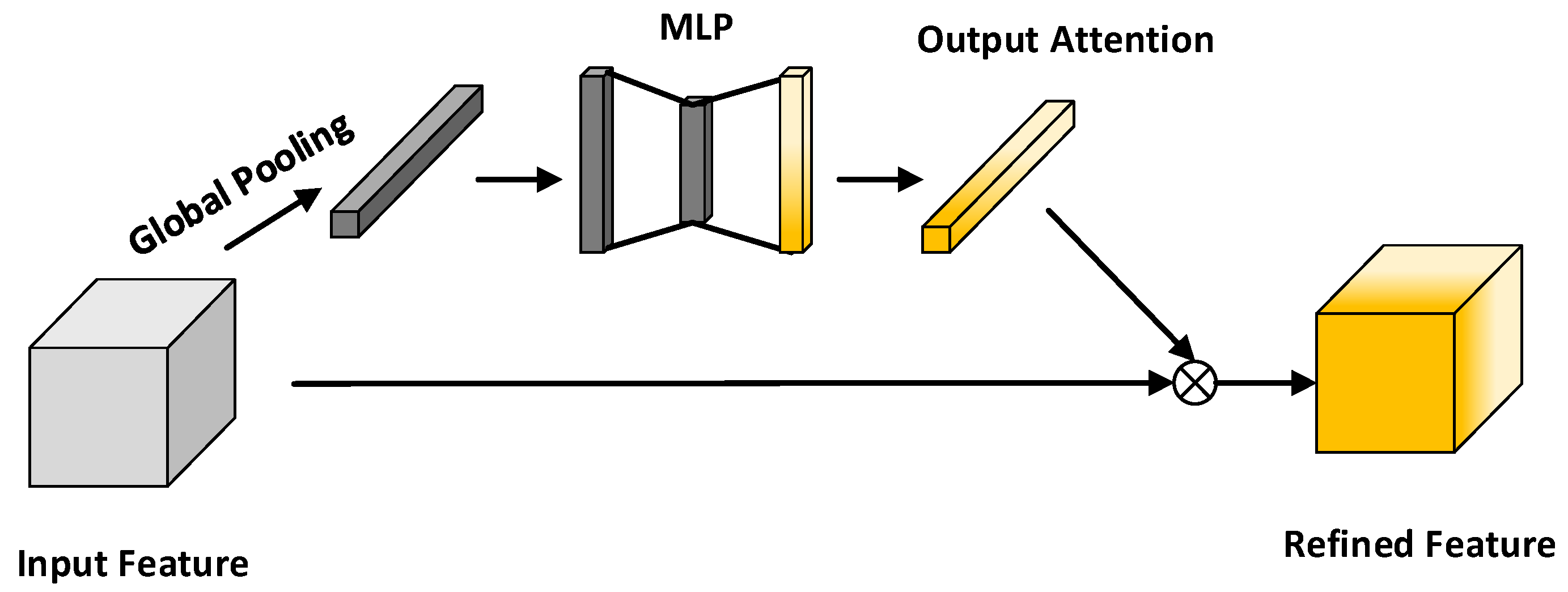
Figure 2 shows the structure of the channel attention module [39]. It exploits the channel interdependencies of the feature mapping, and this module determines which channel is important by calculating the weights. As shown in Figure 3, the channels that have a large impact on the noise reconstruction are given a greater weight. Since the convolutional layer only makes use of local information and not global contextual information, we first use the global average pool to represent the global information that represents the whole image. First, input the feature to obtain the context information in the spatial dimension through global pooling, thereby obtaining a one-dimensional vector .
where is the value at the position of the feature map.
Then, use the vector as the input of a fully connected layer to obtain the description vector , and multiply the input feature and the description vector to obtain the refine feature .
where represents the sigmoid nonlinear activation function, and represent the fully connected layer, the second parameter represents the number of neurons, and represents the element multiplication. The multiplied feature has the same dimension as the input feature.
2.4. Residual Structure
The residual network structure was first proposed by He Kaiming’s team [35]. The residual network was proposed to solve the network degradation problem of deep neural networks (DNN) when there are too many layers. As the number of network layers increases, the accuracy of the network reaches saturation and then rapidly degrades, and this degradation is not caused by overfitting. The skip connection in ResNet solves the problem of gradient disappearance in deep neural networks, allowing gradients to flow through this alternative shortcut. Another way to help with these connections is to allow the model to learn its functions, thus ensuring that the performance of the higher layer is at least the same as the lower layer, not worse. The formula can be expressed as follows:
where is the residual mapping to be learned, is the parameter to be learned, and x is the feature map input by the upper layer.
The network composed of multiple residual learning modules is the residual network. The residual network has been widely used in image classification, target detection, and image super-resolution, and has achieved satisfactory results. In the DnCNN denoising network proposed by Zhang [34], this residual learning idea is also used to improve the performance of the denoising model. For image denoising, the noise image y and the clear image x are usually similar, so the network learning the identity mapping F(y) = x and the residual network directly learning R(y) = y − x will make training easier.
3. Proposed Method
3.1. Network Architecture
Figure 4 shows the overall structure of our proposed RSIDNet. The input is our noisy image, which can be a single-channel panchromatic remote sensing image or a color format remote sensing image . First, through multi-scale feature extraction, in the model, the first layer extracts as many features as possible from the input, expressed as:
where represents an ordinary convolutional layer, the convolution kernel size of this convolutional layer is , the number of output channels is c, represents the non-linear layer ReLU, and BN represents the batch normalization layer.
The main feature mapping part of the model is composed of the same residual attention block, and each block contains two convolutional layers and a channel attention module. The output of each block is connected to the next block and the global fusion module, which helps to deepen the depth of the model to prevent the gradient from disappearing, and through the jump connection, the shallow information extracted by the model is also fused in the subsequent modules.
where represents the output after passing the GFF module, GFF represents the global feature fusion module, F represents the enhanced attention block (ECA), represents the output result of the i-th enhanced attention block (ECA), and n is a hyperparameter representing the number of enhanced attention modules. and represent the convolutional layer and channel attention layer, respectively, in the residual attention module.
3.2. Role of Multi-Scale Feature Extraction Module
Inspired by the inception network structure [20,40], as shown in Figure 5, multi-scale feature extraction is used in the location of feature extraction [41]. Compared with ordinary convolution, the multi-scale network extracts different context information. Specifically, the input goes through four paths, which are convolutional layers with different kernel sizes , and the number of output channels in each output layer is .
After obtaining the output results of the four channels, we aggregate the four output results to obtain a matrix with the number of channels c.
3.3. Loss Function
There are many choices of loss functions for optimization in the field of deep learning image denoising, such as loss function, loss function, perceptual loss function, and total variation loss function [9]. Some networks use multiple loss functions to optimize the model. In this paper, the mean square error (MSE) is selected as the loss function to calculate the difference between the predicted residual image and the corresponding . and represent the noise image and the real image, respectively. It can be expressed as:
represents the parameters of the RSIDNet after training, N represents the number of noisy and clear image pairs, and the Adam optimizer optimizes the parameters to continuously minimize the value of the loss function.
4. Experiments
4.1. Datasets
Our training data use the public dataset NWPU-RESISC45 [42] from Northwestern Polytechnical University. A partial picture of the dataset is shown in Figure 6. The size of each remote sensing image in the dataset is 256 × 256. The dataset contains a total of 45 types of color remote sensing images; for each type of remote sensing, there are 700 images, for a total of 31,500 images. The grayscale image used in the experiment was generated by converting the color image into YCbCr space and then taking the Y component as the gray image. In the experiment, 70% of the dataset was used for training and 30% was used for denoising performance tests. The process of generating a synthetic noise image entails taking out a remote sensing image x in the above training set and adding Gaussian white noise n with standard deviation , thus obtaining a synthetic noise image y, which can be described by the formula:
where the probability density function of the noise n is:
Different noise levels (i.e., = 15, 25, 35, and 50) were used in the experiments for training and testing, and the training results of the training set with noise levels in the interval [0, 55] were used as the results of blind denoising.
To verify the denoising effect of the trained model on other datasets, we randomly selected 50 images in the UCMerceed_LandUse dataset [43] as the test set. For the noisy images used for training, we used the bicubic interpolation method with down factors of 0.7, 0.8, 0.9, and 1 to increase the diversity of the training samples. Because different areas of the image contain different detailed features, we need to divide the training set into small patches of 60 × 60. This can effectively improve the robustness of feature extraction and the efficiency of training models in the denoising process.
4.2. Implementation Details and Hyperparameter Settings
4.2.1. Implementation Settings
Inspired by [44], to speed up the training speed and the limitation of video memory, the training data were divided into a block size of 60 and a step length of 20. In the training process, the initial learning rate was set to , , and the total number of training units was 70. After 20 epochs, the learning rate decayed to one-tenth of the original, and the batch size was set to 32. The parameters of the network were initialized using the method proposed by He et al. [45]; the optimizer uses Adam [46] algorithm and the parameters are .
We used PyTorch version 1.10.1 [47] and Python version 3.7 to train and test the model. The whole experiment has an Intel Core i7-10700K CPU, 32G memory, and NVIDIA GeForce RTX 3070 GPU. The CUDA and CuDNN versions are 11.3 and 8.2.1, respectively.
4.2.2. Network Hyperparameters
In our proposed neural network, two parameters must be manually set. One is the number of enhanced channel attention blocks B and the number of feature channels c. These two parameters also determine the depth of the network. As shown in Figure 7, we compared the effects of different numbers of enhanced attention blocks B and different feature channels c on the denoising performance. The dataset in the experiment is the NWPU-RESISC45 test set with a noise signal of . It can be seen from the figure that as the number of enhanced attention increases, the performance of the model gradually improves. In theory, this is because of the increase in the depth of the model. The nonlinear expression ability of the model is increased, so that complex noise signals can be fitted, but when L > 8, the performance of the model no longer increases significantly, but the amount of calculation is constantly increasing. This is because as the depth of the model increases, the difficulty of training gradually increases, and the model approaches saturation, which may lead to a decline in the learning ability of some shallow information, so the performance of the model no longer improves. In addition, when the number c of feature maps becomes larger and larger, the performance of the model gradually grows slowly, but the amount of parameters is greatly improved. To achieve a balance between computational burden and model performance, we chose c = 64.
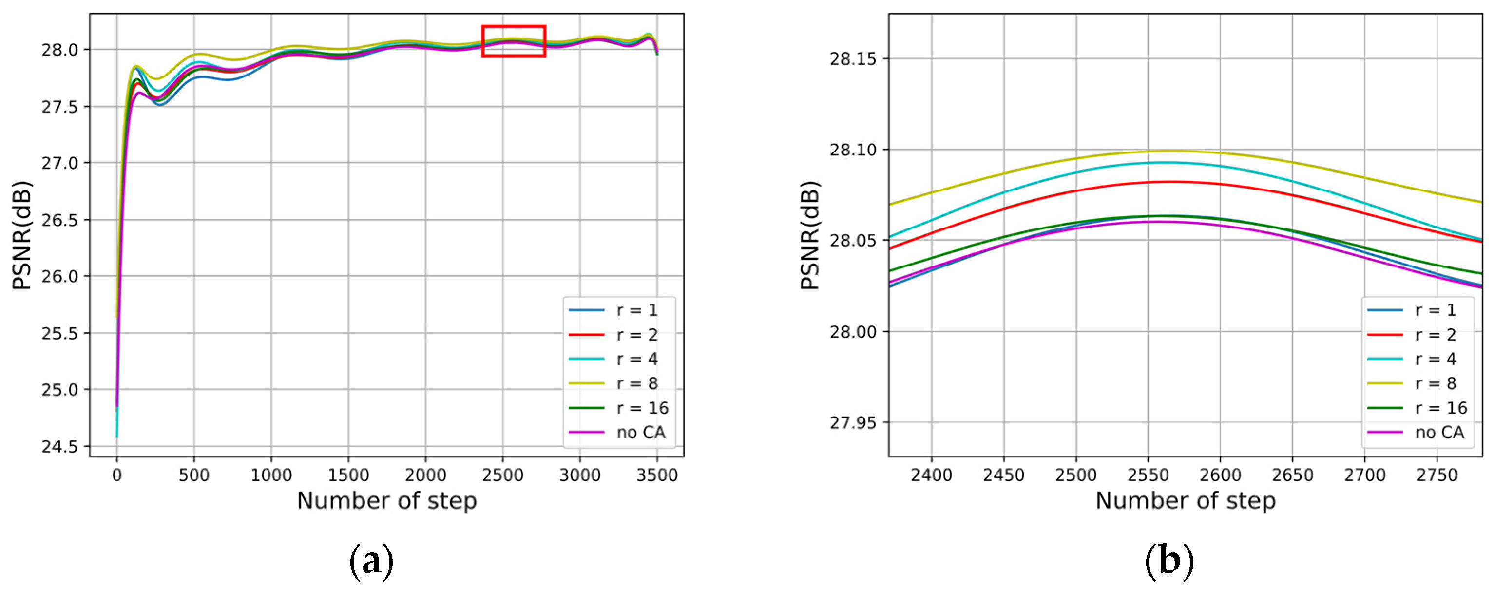
Figure 8 shows the influence of different attenuation coefficients r in channel attention on model denoising performance. When there is no channel attention module, the value of the denoising evaluation index PSNR is the smallest, which shows the effectiveness of adding channel attention. When r = 1, it means that there is no reduction in the dimensionality of the feature vector, but there may be over-fitting problems resulting in poor results on the test set. Later, as the attenuation coefficient r increases, information is lost due to many compressions, so we chose r = 8. In this setting, the model has a better balance between performance and parameters.
4.2.3. Implementation Process
The algorithm implementation process mentioned in this paper is similar to other deep learning-based methods and consists of four main steps: (1) neural network model building, (2) dataset pre-processing, (3) training the model, and (4) prediction of denoised images by the training model.
The detailed design of each process is described in detail below.
(1) Neural network model building: The powerful expressiveness of neural networks and deep learning models is determined by the structure of neural networks and the number of parameters, and the construction of neural network models is an important step in deep learning methods. In Section 3.1 of this paper, we introduce the detailed structure of our proposed RSIDNet, and in Section 4.2, we introduce the hyperparameter settings in the model, and based on these, we can quickly implement the RSIDNet network model and subsequently input the dataset into the model to realize the training of the model, and the neural network framework can automatically select the CPU or GPU according to the configuration of the personal computer. The initial value of the weight matrix of the neural network has a significant impact on the training process and the final results. Therefore, to ensure a suitable performance of the network, we also perform the He initialization operation for the parameters in the RSIDNet model.
(2) Dataset pre-processing: The images in the dataset cannot be directly input to the neural network. There are three steps for pre-processing the training set of remote sensing images, which are image chunking, image pixel value normalization, and data enhancement. The normalization is realized by scaling the pixel values of the images so that the pixel values are between [0, 1], which can be described by the formula:
where represents the value of the i-th pixel in an image; represent the minimum and maximum values of the pixel values in an image, respectively; and represents the value after normalization.
To speed up the training speed and the limitation of video memory, the training data are divided into a block size of 60 and a step length of 20. The bicubic interpolation method with down factors of 0.7, 0.8, 0.9, and 1 is used to achieve data augmentation.
(3) Training model: The detailed settings of the optimizer, loss function, batch size, epoch, learning rate, and other parameters in the model training process are described in Section 4.2 of this paper. The trained model file is then brought to the next step.
(4) Prediction of denoised images by the trained model: This step normalizes the noisy remote sensing image and feeds it into the trained model to obtain a clean remote sensing image.
4.3. Compare with Advanced Algorithms
In this work, we conducted contrast experiments on grayscale and color-synthesized Gaussian noise images. Comparative experiments were carried out on different test datasets. In these experiments, we selected the current state-of-the-art algorithms in the field of traditional remote sensing image denoising and deep learning. These methods include BM3D [27], K-SVD [29], WNNM [24], DnCNN [34], ADNet [48], and ECNDNet [49]. We use two commonly used image restoration indicators, PSNR and SSIM [9], to quantitatively compare the performance of the denoising methods. The following is a detailed description of the performance metrics.
For a given size m × n, clean image I, and denoised image K, the mean square error is defined as follows:
Then, there is PSNR as:
MAX and MSE represent the maximum value of the pixel and the root mean square error between the noisy image and the denoised image, respectively. Generally, for uint8 data, the maximum pixel value is 255; for floating-point data, the maximum pixel value is 1.
The SSIM formula is measured based on the three indicators brightness, contrast, and structure between the denoised image x and the real image y. This evaluation method can be more in line with the perception of the human eye.
where and are the mean values of x and y, respectively; and are the variances of x and y, respectively; is the covariance of x and y; and and are two constants to avoid division by zero.
4.3.1. Gray and Color Synthetic Noisy Remote Sensing Image
In this section, we use qualitative and quantitative methods to illustrate the effectiveness of our proposed method from two aspects: visual perspective and objective evaluation indicators. The quantitative results (PSNR/SSIM) of color and grayscale remote sensing images are shown in Table 1 and Table 2 respectively. All experiments are on the test datasets NWPU-RESISC45 and UCMerced_LandUse under different noise levels (i.e., 15, 25, 35, 50). RSIDNet is very competitive with other popular methods for color and gray noisy images from test datasets. Traditional algorithms such as K-SVD and BM3D reveal the worst results, since traditional methods are not like deep learning methods that can learn prior knowledge from external data for image reconstruction. After denoising, KSVD still has a small part of the noise. Although BM3D effectively removes the noise, it has the problems of excessive smoothness and loss of detail. Other deep learning-based denoising algorithms can retain more detail than BM3D, but the effect is still not ideal. Compared with the above-mentioned methods, our proposed method can not only remove the noise but also retain the detailed texture information in the image, while also achieving better denoising performance.
Figure 9, Figure 10, Figure 11, and Figure 12 illustrate the visual images from K-SVD, BM3D, DnCNN, ECNDNet, and ADNet. It can be seen that our method is significantly ahead of other methods in maintaining image detail and image sharpness. In addition, as shown in Table 3, we experimented with remote sensing images of different scenes. Although these same images have different texture characteristics, contrast, and brightness, increasing the difficulty of denoising, our proposed method achieved competitive results compared to other methods. The advantage of this algorithm is not obvious in images with simple textures or images with less information in them, such as beach and deep forest.
4.3.2. Real Noisy Remote Sensing Images
To further illustrate the effectiveness of our proposed algorithm, we used two real remote sensing images with noise for our experiments. Since these remote sensing images do not have corresponding clean images, the full-reference image quality evaluation is not applicable to our experiments, and therefore, the no-reference image quality assessment [50,51,52] proposed by previous authors was adopted as our evaluation metric.
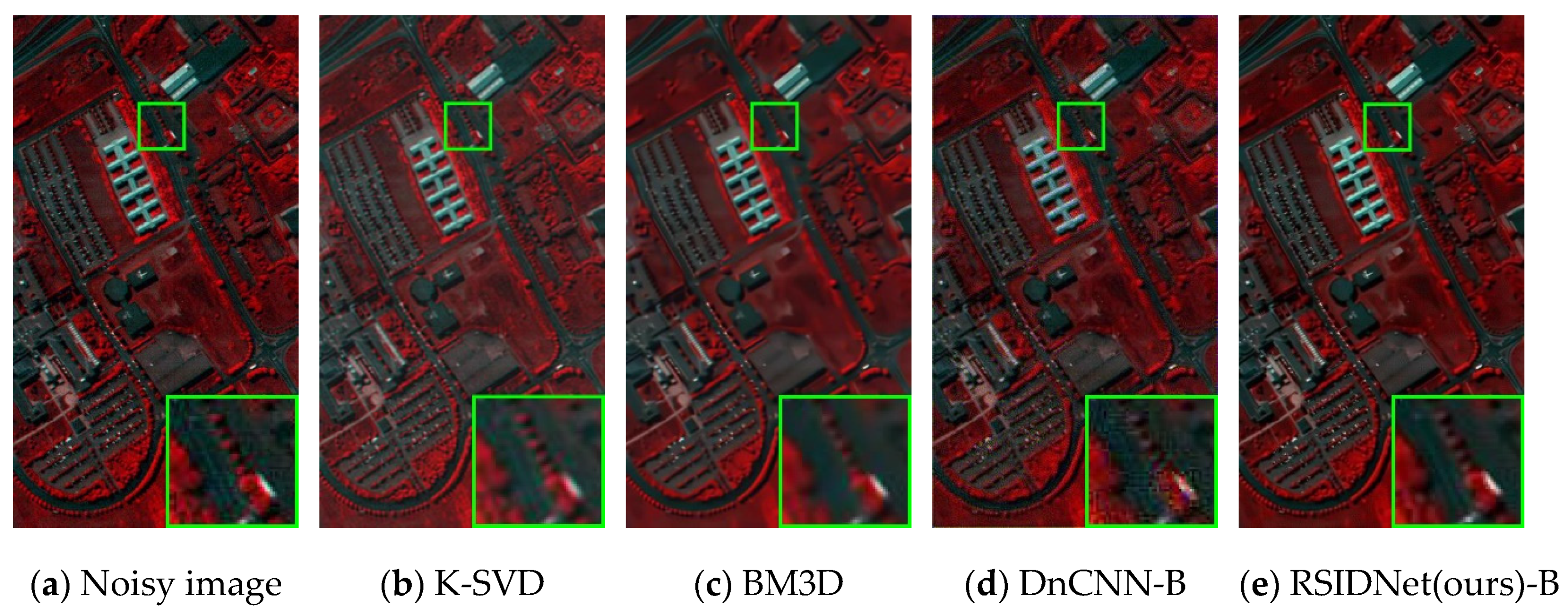
From [53], it can be seen that the first few bands and several other bands of the AVIRIS Indian Pines Dataset are severely affected by Gaussian noise and impulse noise, so the third band of the dataset was extracted as a grayscale image for denoising in our experiments, and for color remote sensing image denoising, we used the ROSIS University of Pavia Dataset’s [54] bands 2, 3, and 97 to synthesize the color images. Figure 13 and Figure 14 compare the denoising results of our proposed algorithm with the visual comparison of the results of other algorithms. Because it is not known exactly what the noise level in the image is, a blind denoising method is used. It can be seen that K-SVD and DnCNN do not remove noise very well and may introduce other artifacts. BM3D efficiently suppresses noise but leads to excessive smoothing. Our proposed method effectively removes noise while retaining some useful detailed textures without over-smoothing the image, and removes noise while preserving the detailed parts.
The results of no-reference image quality evaluation algorithms on denoised images are shown in Table 4, where the Spatial–Spectral Entropy-based Quality (SSEQ) algorithm, which is particularly sensitive to noise, has a higher metric when the noise intensity in the image is high and can be used as an indicator of the content of high-frequency components in the image, and the Blind/Referenceless Image Spatial Quality Evaluator (BRISQUE) is a reference-free algorithm for evaluating image quality in the spatial domain. The overall principle of the algorithm is to extract mean subtracted contrast normalized (MSCN) coefficients from the image, fit the MSCN coefficients to an asymmetric generalized Gaussian distribution (AGGD), and extract the fitted asymmetric generalized image. The blind image integrity notator using DCT Statistics (BLIINDS-II) algorithm first establishes a statistical probability model of the relationship between image features and image quality. The probability distribution is mostly described by a multivariate Gaussian distribution. For the image to be evaluated, the features are extracted and the image quality is calculated with maximum a posteriori probability based on the probability model, or the image quality is estimated based on the match to the probability model (e.g., the distance between features). Although the unreferenced image quality evaluation is not as accurate as the referenced image quality evaluation, it gives a general indication of the quality of the image, and it can be seen that our proposed algorithm has some advantages in these methods.
4.4. Ablation Experiment
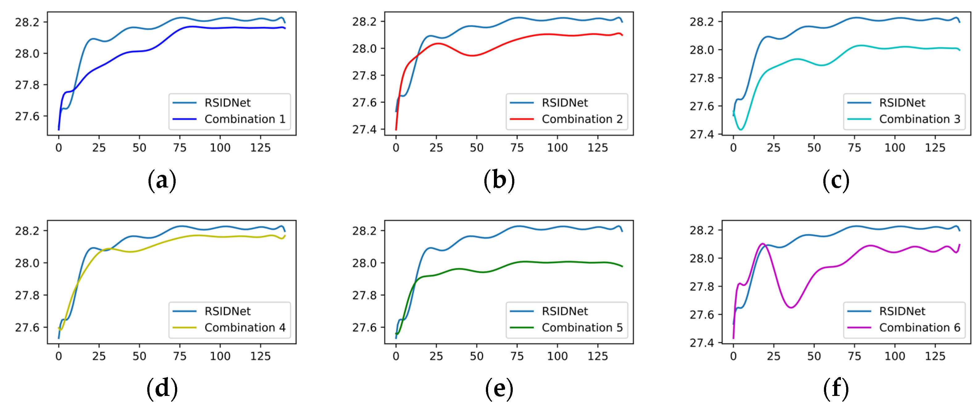
We conducted six ablation experiments to illustrate the importance of the three components in our RSIDNet. All experiments are evaluated on the validation dataset of NWPU-RESISC45. Table 5 shows the average PSNR and SSIM, and the best performance can be achieved when all three components are available. We can see from Table 5 that the lack of any of the following three components in our RSIDNet will have a negative impact on the objective performance metrics of the generated image. Figure 15 uses training curves to compare the performance of RSIDNet with the other six combinations of network architecture. Among them, the attention mechanism shows an important role. In the absence of the attention mechanism, even if the other two components are included, it is still 0.22 dB less than the best PSNR result.
5. Summary and Conclusions
Remote sensing image denoising has been an important research area in the field of remote sensing image processing and computer vision. The process of remote sensing image denoising entails estimating a pure image from the original noisy image so that it can be more in line with the human eye’s perception and facilitate the subsequent remote sensing image processing.
In this paper, we propose a novel denoising network, RSIDNet, based on deep learning methods and taking into account the characteristics of remote sensing images, mainly consisting of a multi-scale feature extraction module (MFE), multiple locally skipped connected enhanced attention blocks (ECA), a global feature fusion block (GFF), and a noisy image reconstruction block (NR). The combination of these blocks greatly improves the model’s use of extracted features and increases the model’s denoising capability. We use a multi-scale feature extraction block in the first layer of the model to extract as many features and detailed textures as possible from the original noisy image, effectively improving the model’s ability to retain detail and the model’s ability to generalize. We fused the deep and shallow information of the model in the main feature mapping section through jump connections in the later network structure, facilitating a staged reconstruction process. The shallow information focuses on local information in the image, such as edges, while the deep information focuses on global information in the image, such as texture and higher-level semantic information, thus improving the expressiveness of the denoising model to obtain a satisfactory noise feature map. The attention enhancement module is specifically designed for processing remote sensing images with complex information. The module is capable of mining noise information hidden in complex backgrounds from a given noisy image and is significantly useful for processing complex noisy images.
In this work, a series of experiments were conducted to analyze and validate the performance of the proposed algorithm. Firstly, the effectiveness of the proposed method was verified on different datasets, including traditional image denoising algorithms and the latest deep learning-based algorithms. The experimental results show that the algorithms in this paper achieve a leading position in terms of denoising capability on both gray and color images, both in terms of objective evaluation metrics and visual effect comparison. The generated images can retain a large amount of texture details compared to other methods, and stable results were achieved when the trained models were tested on different datasets. Moreover, as the noise intensity increases, the algorithm in this paper has a more obvious improvement compared to other algorithms. To further illustrate the effectiveness of the proposed algorithm, two real remote sensing images with noise were used for testing. Excellent results were also achieved in the quality evaluation of the unreferenced images compared to other methods. Finally, the effectiveness of several modules mentioned in this paper is demonstrated by ablation experiments. Through extensive experiments, we demonstrate that our proposed RSIDNet achieves satisfactory results in terms of objective metrics and high-quality denoising of remotely sensed images.
Convolutional neural network-based image denoising has made unprecedented breakthroughs in recent years, but most of the current methods are based on simple image degradation models for remote sensing images, where real remote sensing images with noise may be affected by multiple external signals. In our future planning, we will study how to generate noise maps from noisy images and then build datasets by simulating noise. Additionally, we will use our strengths to produce a standard real remote sensing image denoising dataset in collaboration with relevant units. Although our model has achieved excellent results in recovering image quality, there are limitations in its current application. First, our model is more complex than other deep learning-based methods. Model inference on a graphics processing unit (GPU) can be very fast but is not very effective when using only a central processing unit (CPU). In the future, we will investigate our model to compress and simplify the processing without losing denoising performance. The training and testing of the remote sensing image denoising algorithms mentioned in this paper are based on computer platforms. Porting and integrating algorithms based on some new deep learning hardware devices, such as Nvidia’s Jetson TX2 development board and the Movidius Neural Compute Stick, are important next steps for practical applications.
Author Contributions
All authors were involved in the formulation of the problem and the design of the methodology; L.H. designed the experiment and wrote the manuscript; H.L. (Hailong Liu) and G.B. analyzed the accuracy of the experimental data; Y.Z. (Yuchen Zhao) and H.L. (Hengyi Lv) reviewed and guided the paper. Y.Z. (Yisa Zhang) made the data curation. All authors have read and agreed to the published version of the manuscript.
Funding
This research was funded by the National Natural Science Foundation of China (62005269).
Acknowledgments
The authors thank the editors and reviewers for their hard work and valuable advice.
Conflicts of Interest
The authors declare no conflict of interest.
References
- Feng, X.B.; Zhang, W.X.; Su, X.Q.; Xu, Z.P. Optical Remote Sensing Image Denoising and Super-Resolution Reconstructing Using Optimized Generative Network in Wavelet Transform Domain. Remote Sens. 2021, 13, 1858. [Google Scholar] [CrossRef]
- Zhu, Y.H.; Yang, G.J.; Yang, H.; Zhao, F.; Han, S.Y.; Chen, R.Q.; Zhang, C.J.; Yang, X.D.; Liu, M.; Cheng, J.P.; et al. Estimation of Apple Flowering Frost Loss for Fruit Yield Based on Gridded Meteorological and Remote Sensing Data in Luochuan, Shaanxi Province, China. Remote Sens. 2021, 13, 1630. [Google Scholar] [CrossRef]
- Qi, J.H.; Wan, P.C.; Gong, Z.Q.; Xue, W.; Yao, A.H.; Liu, X.Y.; Zhong, P. A Self-Improving Framework for Joint Depth Estimation and Underwater Target Detection from Hyperspectral Imagery. Remote Sens. 2021, 13, 1721. [Google Scholar] [CrossRef]
- Zhang, J.Y.; Zhang, X.R.; Tang, X.; Huang, Z.J.; Jiao, L.C. Vehicle Detection and Tracking in Remote Sensing Satellite Vidio Based on Dynamic Association. In Proceedings of the 10th International Workshop on the Analysis of Multitemporal Remote Sensing Images (MultiTemp), Shanghai, China, 5–7 August 2019. [Google Scholar]
- Xia, J.Q.; Wang, Y.Z.; Zhou, M.R.; Deng, S.S.; Li, Z.W.; Wang, Z.H. Variations in Channel Centerline Migration Rate and Intensity of a Braided Reach in the Lower Yellow River. Remote Sens. 2021, 13, 1680. [Google Scholar] [CrossRef]
- Yuan, Q.Q.; Zhang, Q.; Li, J.; Shen, H.F.; Zhang, L.P. Hyperspectral Image Denoising Employing a Spatial-Spectral Deep Residual Convolutional Neural Network. IEEE Trans. Geosci. Remote Sens. 2019, 57, 1205–1218. [Google Scholar] [CrossRef] [Green Version]
- Gao, F.; Huang, T.; Sun, J.P.; Wang, J.; Hussain, A.; Yang, E.F. A New Algorithm for SAR Image Target Recognition Based on an Improved Deep Convolutional Neural Network. Cogn. Comput. 2019, 11, 809–824. [Google Scholar] [CrossRef] [Green Version]
- Landgrebe, D.A.; Malaret, E. Noise in Remote-Sensing Systems—The Effect on Classification Error. IEEE Trans. Geosci. Remote Sens. 1986, 24, 294–300. [Google Scholar] [CrossRef]
- Tian, C.W.; Fei, L.K.; Zheng, W.X.; Xu, Y.; Zuo, W.M.; Lin, C.W. Deep learning on image denoising: An overview. Neural Netw. 2020, 131, 251–275. [Google Scholar] [CrossRef]
- Anwar, S.; Barnes, N. Real Image Denoising with Feature Attention. In Proceedings of the IEEE/CVF International Conference on Computer Vision (ICCV), Seoul, Korea, 27 October–2 November 2019; pp. 3155–3164. [Google Scholar]
- Xue, S.K.; Qiu, W.Y.; Liu, F.; Jin, X.Y. Wavelet-based residual attention network for image super-resolution. Neurocomputing 2020, 382, 116–126. [Google Scholar] [CrossRef]
- Goyal, B.; Dogra, A.; Agrawal, S.; Sohi, B.S.; Sharma, A. Image denoising review: From classical to state-of-the-art approaches. Inf. Fusion 2020, 55, 220–244. [Google Scholar] [CrossRef]
- Singh, L.; Janghel, R. Image Denoising Techniques: A Brief Survey. In Proceedings of the 4th International Conference on Harmony Search, Soft Computing and Applications (ICHSA), BML Munjal Univ, Sidhrawali, India, 7–9 February 2018; pp. 731–740. [Google Scholar]
- Foi, A.; Trimeche, M.; Katkovnik, V.; Egiazarian, K. Practical Poissonian-Gaussian noise modeling and fitting for single-image raw-data. IEEE Trans. Image Process. 2008, 17, 1737–1754. [Google Scholar] [CrossRef] [PubMed] [Green Version]
- Zhang, M.H.; Zhang, F.Q.; Liu, Q.G.; Wang, S.S. VST-Net: Variance-stabilizing transformation inspired network for Poisson denoising. J. Vis. Commun. Image Represent. 2019, 62, 12–22. [Google Scholar] [CrossRef]
- Chen, J.W.; Chen, J.W.; Chao, H.Y.; Yang, M. Image Blind Denoising with Generative Adversarial Network Based Noise Modeling. In Proceedings of the 31st IEEE/CVF Conference on Computer Vision and Pattern Recognition (CVPR), Salt Lake City, UT, USA, 18–23 June 2018; pp. 3155–3164. [Google Scholar]
- Cha, S.; Park, T.; Kim, B.; Baek, J.; Moon, T.J. GAN2GAN: Generative Noise Learning for Blind Denoising with Single Noisy Images. arXiv 2019, arXiv:1905.10488. [Google Scholar]
- Huang, T.; Li, S.; Jia, X.; Lu, H.; Liu, J.J. Neighbor2Neighbor: Self-Supervised Denoising from Single Noisy Images. arXiv 2021, arXiv:2101.02824. [Google Scholar]
- Pang, T.; Zheng, H.; Quan, Y.; Ji, H. Recorrupted-to-Recorrupted: Unsupervised Deep Learning for Image Denoising. In Proceedings of the IEEE/CVF Conference on Computer Vision and Pattern Recognition(CVPR), Nashville, TN, USA, 20–25 June 2021; pp. 2043–2052. [Google Scholar]
- Szegedy, C.; Liu, W.; Jia, Y.Q.; Sermanet, P.; Reed, S.; Anguelov, D.; Erhan, D.; Vanhoucke, V.; Rabinovich, A. Going Deeper with Convolutions. In Proceedings of the IEEE Conference on Computer Vision and Pattern Recognition (CVPR), Boston, MA, USA, 7–12 June 2015; pp. 1–9. [Google Scholar]
- Rudin, L.I.; Osher, S.; Fatemi, E. Nonlinear Total Variation Based Noise Removal Algorithms. Physica D 1992, 60, 259–268. [Google Scholar] [CrossRef]
- Yihu, C.; Zhenglin, Y.E. Improved anisotropic diffusion image denoising method. Comput. Eng. Appl. 2008, 44, 170–172. [Google Scholar]
- Buades, A.; Coll, B.; Morel, J.M. Nonlocal image and movie denoising. Int. J. Comput. Vis. 2008, 76, 123–139. [Google Scholar] [CrossRef]
- Gu, S.H.; Zhang, L.; Zuo, W.M.; Feng, X.C. Weighted Nuclear Norm Minimization with Application to Image Denoising. In Proceedings of the 27th IEEE Conference on Computer Vision and Pattern Recognition (CVPR), Columbus, OH, USA, 23–28 June 2014; pp. 2862–2869. [Google Scholar]
- Donoho, D.L.; Johnstone, I.M. Ideal Spatial Adaptation by Wavelet Shrinkage. Biometrika 1994, 81, 425–455. [Google Scholar] [CrossRef]
- Gai, S.; Bao, Z.Y.; Zhang, K.G. Vector extension of quaternion wavelet transform and its application to colour image denoising. IET Signal Process. 2019, 13, 133–140. [Google Scholar] [CrossRef]
- Dabov, K.; Foi, A.; Katkovnik, V.; Egiazarian, K. Image denoising by sparse 3-D transform-domain collaborative filtering. IEEE Trans. Image Process. 2007, 16, 2080–2095. [Google Scholar] [CrossRef]
- Lewicki, G.; Marino, G. Approximation by superpositions of a sigmoidal function. Z. Anal. Ihre. Anwend. 2003, 22, 463–470. [Google Scholar] [CrossRef] [Green Version]
- Aharon, M.; Elad, M.; Bruckstein, A. K-SVD: An algorithm for designing overcomplete dictionaries for sparse representation. IEEE Trans. Signal Process. 2006, 54, 4311–4322. [Google Scholar] [CrossRef]
- Zhao, H.H.; Luo, J.; Huang, Z.H.; Nagumo, T.; Murayama, J.; Zhang, L.Q. Statistically Adaptive Image Denoising Based on Overcomplete Topographic Sparse Coding. Neural Process. Lett. 2015, 41, 357–369. [Google Scholar] [CrossRef]
- Burger, H.C.; Schuler, C.J.; Harmeling, S. Image denoising: Can plain neural networks compete with BM3D? In Proceedings of the 2012 IEEE conference on computer vision and pattern recognition(CVPR), Providence, RI, USA, 16-21 June 2012; pp. 2392–2399. [Google Scholar]
- Chen, Y.J.; Yu, W.; Pock, T. On learning optimized reaction diffusion processes for effective image restoration. In Proceedings of the IEEE Conference on Computer Vision and Pattern Recognition (CVPR), Boston, MA, USA, 7–12 June 2015; pp. 5261–5269. [Google Scholar]
- Jain, V.; Seung, S.J.A. Natural image denoising with convolutional networks. In Proceedings of the 21st International Conference on Neural Information Processing Systems (NIPS), Vancouver, Canada, 8–10 December 2008; pp. 769–776. [Google Scholar]
- Zhang, K.; Zuo, W.M.; Chen, Y.J.; Meng, D.Y.; Zhang, L. Beyond a Gaussian Denoiser: Residual Learning of Deep CNN for Image Denoising. IEEE Trans. Image Process. 2017, 26, 3142–3155. [Google Scholar] [CrossRef] [Green Version]
- He, K.M.; Zhang, X.Y.; Ren, S.Q.; Sun, J. Deep Residual Learning for Image Recognition. In Proceedings of the 2016 IEEE Conference on Computer Vision and Pattern Recognition (CVPR), Seattle, WA, USA, 27–30 June 2016; pp. 770–778. [Google Scholar]
- Ioffe, S.; Szegedy, C. Batch Normalization: Accelerating Deep Network Training by Reducing Internal Covariate Shift. In Proceedings of the 32nd International Conference on Machine Learning, Lille, France, 7–9 July 2015; pp. 448–456. [Google Scholar]
- Zhang, K.; Zuo, W.M.; Zhang, L. FFDNet: Toward a Fast and Flexible Solution for CNN-Based Image Denoising. IEEE Trans. Image Process. 2018, 27, 4608–4622. [Google Scholar] [CrossRef] [Green Version]
- Divakar, N.; Babu, R.V. Image Denoising via CNNs: An Adversarial Approach. In Proceedings of the 30th IEEE/CVF Conference on Computer Vision and Pattern Recognition Workshops (CVPRW), Honolulu, HI, USA, 21–26 July 2017; pp. 1076–1083. [Google Scholar]
- Hu, J.; Shen, L.; Sun, G. Squeeze-and-Excitation Networks. In Proceedings of the 31st IEEE/CVF Conference on Computer Vision and Pattern Recognition (CVPR), Salt Lake City, UT, USA, 18–23 June 2018; pp. 7132–7141. [Google Scholar]
- Varga, D. Multi-pooled Inception Features for No-reference Video Quality Assessment. In Proceedings of the 15th International Joint Conference on Computer Vision, Imaging and Computer Graphics Theory and Applications (VISIGRAPP)/15th International Conference on Computer Vision Theory and Applications (VISAPP), Valletta, Malta, 27–29 February 2020; pp. 338–347. [Google Scholar]
- Yuan, B.H.; Li, S.J.; Li, N. Multiscale deep features learning for land-use scene recognition. J. Appl. Remote Sens. 2018, 12, 12. [Google Scholar] [CrossRef]
- Cheng, G.; Han, J.W.; Lu, X.Q. Remote Sensing Image Scene Classification: Benchmark and State of the Art. Proc. IEEE 2017, 105, 1865–1883. [Google Scholar] [CrossRef] [Green Version]
- Yang, Y.; Newsam, S. Bag-of-visual-words and spatial extensions for land-use classification. In Proceedings of the 18th SIGSPATIAL International Conference on Advances in Geographic Information Systems, San Jose, CA, USA, 2–5 November 2010; pp. 270–279. [Google Scholar]
- Zoran, D.; Weiss, Y. From Learning Models of Natural Image Patches to Whole Image Restoration. In Proceedings of the IEEE International Conference on Computer Vision (ICCV), Barcelona, Spain, 6–13 November 2011; pp. 479–486. [Google Scholar]
- He, K.M.; Zhang, X.Y.; Ren, S.Q.; Sun, J. Delving Deep into Rectifiers: Surpassing Human-Level Performance on ImageNet Classification. In Proceedings of the IEEE International Conference on Computer Vision, Santiago, Chile, 11–18 December 2015; pp. 1026–1034. [Google Scholar]
- Kingma, D.P.; Ba, J.J. Adam: A method for stochastic optimization. arXiv 2014, arXiv:1412.6980. [Google Scholar]
- Paszke, A.; Gross, S.; Massa, F.; Lerer, A.; Bradbury, J.; Chanan, G.; Killeen, T.; Lin, Z.M.; Gimelshein, N.; Antiga, L.; et al. PyTorch: An Imperative Style, High-Performance Deep Learning Library. In Proceedings of the 33rd Conference on Neural Information Processing Systems (NeurIPS), Vancouver, BC, Canada, 8–14 December 2019. [Google Scholar]
- Tian, C.W.; Xu, Y.; Li, Z.Y.; Zuo, W.M.; Fei, L.K.; Liu, H. Attention-guided CNN for image denoising. Neural Netw. 2020, 124, 117–129. [Google Scholar] [CrossRef]
- Tian, C.W.; Xu, Y.; Fei, L.K.; Wang, J.Q.; Wen, J.; Luo, N. Enhanced CNN for image denoising. CAAI T. Intell. Technol. 2019, 4, 17–23. [Google Scholar] [CrossRef]
- Liu, L.X.; Liu, B.; Huang, H.; Bovik, A.C. No-reference image quality assessment based on spatial and spectral entropies. Signal Process. Image Commun. 2014, 29, 856–863. [Google Scholar] [CrossRef]
- Saad, M.A.; Bovik, A.C.; Charrier, C. Blind Image Quality Assessment: A Natural Scene Statistics Approach in the DCT Domain. IEEE Trans. Image Process. 2012, 21, 3339–3352. [Google Scholar] [CrossRef] [PubMed]
- Mittal, A.; Moorthy, A.K.; Bovik, A.C. No-Reference Image Quality Assessment in the Spatial Domain. IEEE Trans. Image Process. 2012, 21, 4695–4708. [Google Scholar] [CrossRef] [PubMed]
- Chen, Y.Y.; Guo, Y.W.; Wang, Y.L.; Wang, D.; Peng, C.; He, G.P. Denoising of Hyperspectral Images Using Nonconvex Low Rank Matrix Approximation. IEEE Trans. Geosci. Remote Sens. 2017, 55, 5366–5380. [Google Scholar] [CrossRef]
- Bigdeli, B.; Samadzadegan, F.; Reinartz, P. A Multiple SVM System for Classification of Hyperspectral Remote Sensing Data. J. Indian Soc. Remote Sens. 2013, 41, 763–776. [Google Scholar] [CrossRef] [Green Version]
Figure 1.
The general flow of the deep learning denoising method.

Figure 2.
Schematic diagram of attention mechanism.

Figure 3.
We input the picture into the trained model and extracted the different attention values corresponding to the 64 channels in the 7th enhanced attention block, and the heat maps of the corresponding partial feature maps were output after the attention mechanism.
Figure 3.
We input the picture into the trained model and extracted the different attention values corresponding to the 64 channels in the 7th enhanced attention block, and the heat maps of the corresponding partial feature maps were output after the attention mechanism.

Figure 4.
The proposed remote sensing image denoising network consists of four parts, which are a multi-feature extraction module (MFE), an enhance channel attention block (ECA) group, a global feature fusion block (GFF), and a noise feature map reconstruction block (NR).
Figure 4.
The proposed remote sensing image denoising network consists of four parts, which are a multi-feature extraction module (MFE), an enhance channel attention block (ECA) group, a global feature fusion block (GFF), and a noise feature map reconstruction block (NR).

Figure 5.
Schematic diagram of the multi-scale feature extraction used in this paper. The input has four branches, and convolutions with different convolution kernel sizes are performed. The four images on the right are the heat maps of the features extracted in the output of each branch.
Figure 5.
Schematic diagram of the multi-scale feature extraction used in this paper. The input has four branches, and convolutions with different convolution kernel sizes are performed. The four images on the right are the heat maps of the features extracted in the output of each branch.

Figure 6.
Some category images of the NWPU-RESISC45 dataset.

Figure 7.
The influence of the number of different feature maps c and the number of enhanced channel attention blocks (ECA) B on the PSNR results. This experiment is on the NWPU-RESISC45 test set with a noise intensity of .
Figure 7.
The influence of the number of different feature maps c and the number of enhanced channel attention blocks (ECA) B on the PSNR results. This experiment is on the NWPU-RESISC45 test set with a noise intensity of .

Figure 8.
(a) The PSNR result of the channel attention mechanism corresponding to different attenuation coefficients as the number of steps increases. This experiment is on the NWPU-RESISC45 test set with a noise intensity of 35. (b) Enlarged view of the partial area in (a).
Figure 8.
(a) The PSNR result of the channel attention mechanism corresponding to different attenuation coefficients as the number of steps increases. This experiment is on the NWPU-RESISC45 test set with a noise intensity of 35. (b) Enlarged view of the partial area in (a).

Figure 9.
The denoising effects of various methods when the noise intensity is . The PSNR values are: (b) noisy image, 17.87 dB; (c) K-SVD, 23.31 dB; (d) BM3D, 24.39 dB; (e) DnCNN, 25.28 dB; (f) ADNet, 25.34 dB; (g) ECNDNet, 25.30 dB; (h) RSIDNet(ours), 25.38 dB.
Figure 9.
The denoising effects of various methods when the noise intensity is . The PSNR values are: (b) noisy image, 17.87 dB; (c) K-SVD, 23.31 dB; (d) BM3D, 24.39 dB; (e) DnCNN, 25.28 dB; (f) ADNet, 25.34 dB; (g) ECNDNet, 25.30 dB; (h) RSIDNet(ours), 25.38 dB.

Figure 10.
The denoising effects of various methods when the noise intensity is . The PSNR values are: (b) noisy image, 14.72 dB; (c) K-SVD, 21.31 dB; (d) BM3D, 22.94 dB; (e) DnCNN, 23.74 dB; (f) ADNet, 23.79 dB; (g) ECNDNet, 23.81 dB; (h) RSIDNet(ours), 23.88 dB.
Figure 10.
The denoising effects of various methods when the noise intensity is . The PSNR values are: (b) noisy image, 14.72 dB; (c) K-SVD, 21.31 dB; (d) BM3D, 22.94 dB; (e) DnCNN, 23.74 dB; (f) ADNet, 23.79 dB; (g) ECNDNet, 23.81 dB; (h) RSIDNet(ours), 23.88 dB.

Figure 11.
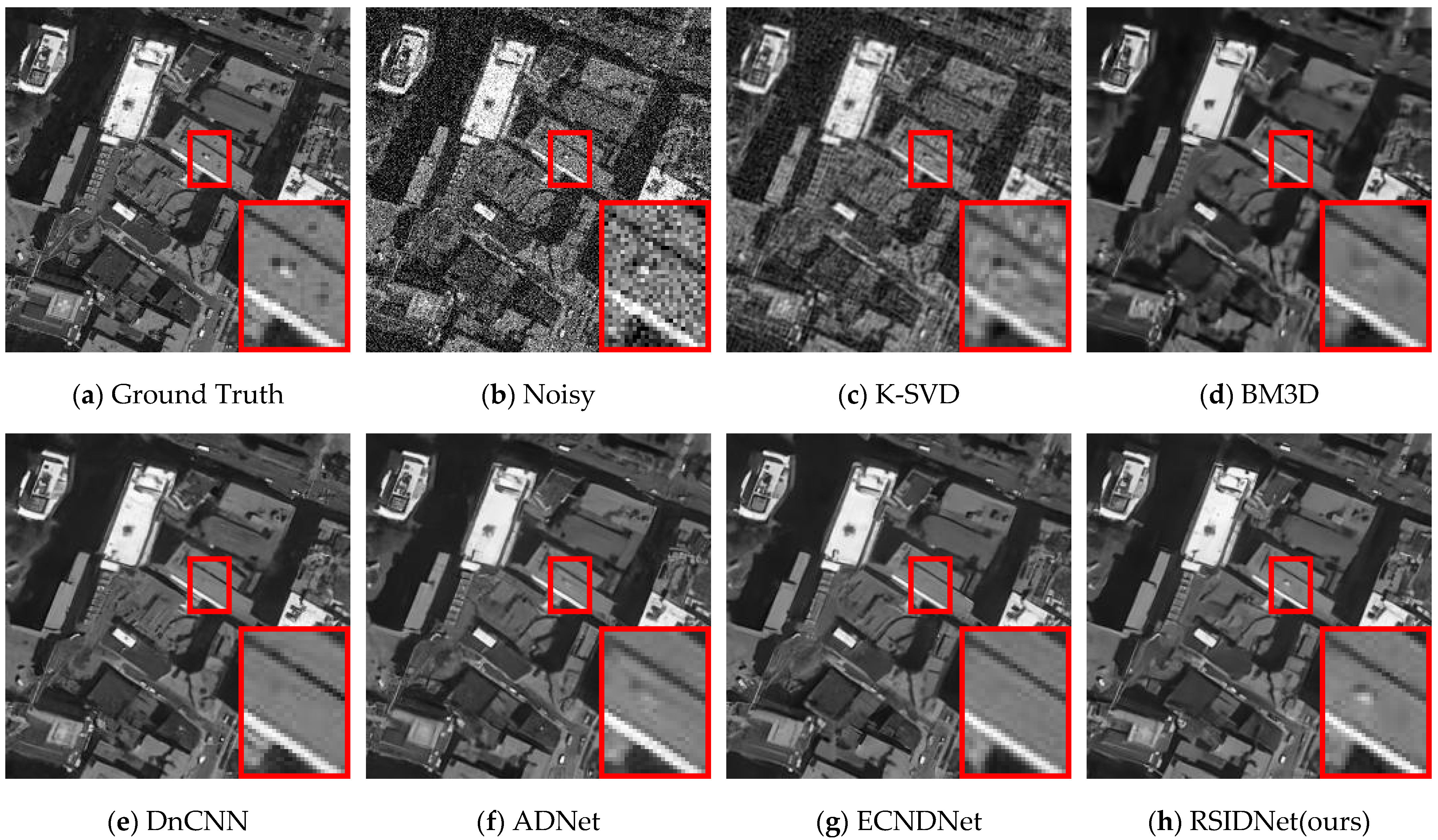
The denoising effects of various methods when the noise intensity is . The PSNR values are: (b) noisy image, 14.81 dB; (c) K-SVD, 24.76 dB; (d) BM3D, 27.03 dB; (e) DnCNN, 27.97 dB; (f) ADNet, 27.95 dB; (g) ECNDNet, 27.96 dB; (h) RSIDNet(ours), 28.11 dB.
Figure 11.
The denoising effects of various methods when the noise intensity is . The PSNR values are: (b) noisy image, 14.81 dB; (c) K-SVD, 24.76 dB; (d) BM3D, 27.03 dB; (e) DnCNN, 27.97 dB; (f) ADNet, 27.95 dB; (g) ECNDNet, 27.96 dB; (h) RSIDNet(ours), 28.11 dB.

Figure 12.
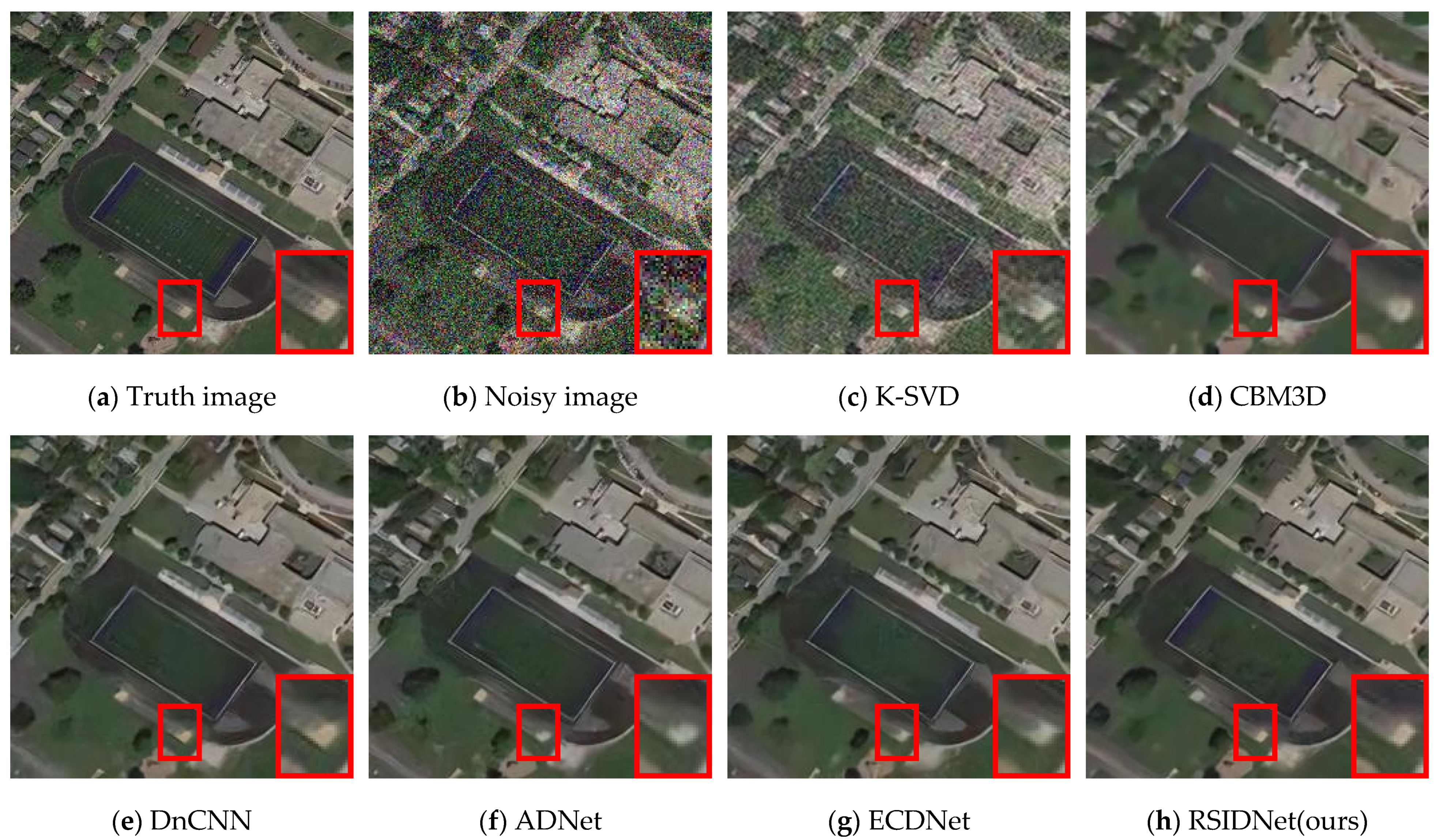
The denoising effect of various methods when the noise intensity is . The PSNR values are: (b) noisy image, 14.55 dB; (c) K-SVD, 24.35 dB; (d) BM3D, 27.04 dB; (e) DnCNN, 28.04 dB; (f) ADNet, 28.06 dB; (g) ECNDNet, 28.01 dB; (h) RSIDNet(ours), 28.13 dB.
Figure 12.
The denoising effect of various methods when the noise intensity is . The PSNR values are: (b) noisy image, 14.55 dB; (c) K-SVD, 24.35 dB; (d) BM3D, 27.04 dB; (e) DnCNN, 28.04 dB; (f) ADNet, 28.06 dB; (g) ECNDNet, 28.01 dB; (h) RSIDNet(ours), 28.13 dB.

Figure 13.
Visual comparison of different methods of denoising on band 3 of the AVIRIS Indian Pines dataset.
Figure 13.
Visual comparison of different methods of denoising on band 3 of the AVIRIS Indian Pines dataset.

Figure 14.
Results for the Pavia University image. (a) Pseudo-color image with bands (2, 3, 97). (b) K-SVD. (c) CBM3D. (d) DnCNN-B. (e) proposed RSIDNet-B.
Figure 14.
Results for the Pavia University image. (a) Pseudo-color image with bands (2, 3, 97). (b) K-SVD. (c) CBM3D. (d) DnCNN-B. (e) proposed RSIDNet-B.

Figure 15.
Comparison of the training curves of six different combinations of network architecture with the RSIDNet, where the horizontal coordinate represents the number of steps and the vertical coordinate represents the PSNR. (a–f) represent the respective training curves of the network structure combinations 1–6 compared to the training curves of RSIDNet.


Table 1.
Different noise levels and blind denoising performance metrics in the NWPU-RESISC45 and UCMerced_LandUse datasets.
Table 1.
Different noise levels and blind denoising performance metrics in the NWPU-RESISC45 and UCMerced_LandUse datasets.
| Dataset | Methods | σ = 15 PSNR/SSIM | σ = 25 PSNR/SSIM | σ = 35 PSNR/SSIM | σ = 50 PSNR/SSIM |
|---|---|---|---|---|---|
| NWPU-RESISC45 | BM3D | 31.52/0.9316 | 29.05/0.8862 | 27.49/0.8470 | 25.82/0.7977 |
| K-SVD | 29.42/0.8950 | 26.89/0.8146 | 24.56/0.7295 | 22.59/0.6171 | |
| WNNM | 31.44/0.8509 | 29.38/0.8030 | 27.97/0.7515 | 26.54/0.6972 | |
| DnCNN-S | 31.90/0.9345 | 29.51/0.8934 | 28.13/0.8596 | 26.71/0.8158 | |
| DnCNN-B | 31.80/0.9332 | 29.49/0.8924 | 28.07/0.8575 | 26.65/0.8154 | |
| ADNet | 31.83/0.9367 | 29.53/0.8990 | 28.11/0.8655 | 26.71/0.8260 | |
| ECNDNet | 31.72/0.9363 | 29.36/0.8936 | 28.10/0.8660 | 26.74/0.8273 | |
| RSIDNet(ours)-S | 31.94/0.9385 | 29.64/0.9007 | 28.22/0.8692 | 26.82/0.8295 | |
| RSIDNet(ours)-B | 31.81/0.9357 | 29.50/0.8964 | 28.03/0.8628 | 26.60/0.8187 | |
| UCMerced_LandUse | BM3D | 31.31/0.9361 | 28.779/0.8935 | 27.18/0.8564 | 25.43/0.8081 |
| K-SVD | 29.31/0.9007 | 26.50/0.8193 | 24.38/0.7357 | 22.06/0.6257 | |
| WNNM | 31.55/0.8822 | 28.99/0.8174 | 27.42/0.7627 | 25.88/0.7047 | |
| DnCNN-S | 31.79/0.9422 | 29.28/0.9046 | 27.72/0.8717 | 26.13/0.8289 | |
| DnCNN-B | 31.52/0.9380 | 29.05/0.8990 | 27.57/0.8661 | 25.85/0.8204 | |
| ADNet | 31.64/0.9402 | 29.19/0.9041 | 27.66/0.8710 | 26.19/0.8298 | |
| ECNDNet | 31.60/0.9394 | 29.08/0.8990 | 27.60/0.8704 | 26.22/0.8314 | |
| RSIDNet(ours)-S | 31.84/0.9429 | 29.38/0.9065 | 27.88/0.8757 | 26.34/0.8353 | |
| RSIDNet(ours)-B | 31.57/0.9384 | 29.10/0.8998 | 27.56/0.8661 | 25.92/0.8212 |
Table 2.
Different noise levels in the RGB color space and blind denoising performance metrics in the NWPU-RESISC45 and UCMeced_LandUse datasets.
Table 2.
Different noise levels in the RGB color space and blind denoising performance metrics in the NWPU-RESISC45 and UCMeced_LandUse datasets.
| Dataset | Methods | σ = 15 PSNR/SSIM | σ = 25 PSNR/SSIM | σ = 35 PSNR/SSIM | σ = 50 PSNR/SSIM |
|---|---|---|---|---|---|
| NWPU-RESISC45 | CBM3D | 33.95/0.9602 | 31.16/0.9277 | 29.32/0.8953 | 27.23/0.8499 |
| K-SVD | 31.05/0.9186 | 28.34/0.8776 | 26.96/0.8205 | 24.68/0.7363 | |
| WNNM | 31.45/0.8508 | 29.35/0.8035 | 27.99/0.7512 | 26.56/0.6974 | |
| DnCNN-S | 34.25/0.9631 | 31.59/0.9356 | 30.00/0.9107 | 28.41/0.8777 | |
| DnCNN-B | 33.98/0.9610 | 31.40/0.9347 | 29.81/0.9090 | 28.30/0.8742 | |
| ADNet | 34.14/0.9621 | 31.54/0.9347 | 29.95/0.9097 | 28.40/0.8774 | |
| ECNDNet | 34.01/0.9602 | 31.36/0.9330 | 29.83/0.9076 | 28.34/0.8755 | |
| RSIDNet(ours)-S | 34.28/0.9635 | 31.61/0.9360 | 30.08/0.9137 | 28.49/0.8791 | |
| RSIDNet(ours)-B | 33.76/0.9602 | 31.44/0.9331 | 29.74/0.9050 | 28.33/0.8741 | |
| UCMerced_LandUse | CBM3D | 33.22/0.9585 | 30.67/0.9299 | 28.97/0.9015 | 27.05/0.8609 |
| K-SVD | 30.85/0.9319 | 28.58/0.8867 | 26.68/0.8333 | 24.46/0.7534 | |
| WNNM | 31.54/0.8820 | 29.95/0.8175 | 27.45/0.7620 | 25.87/0.7052 | |
| DnCNN-S | 33.18/0.9602 | 30.79/0.9347 | 29.29/0.9105 | 27.70/0.8774 | |
| DnCNN-B | 32.94/0.9589 | 30.65/0.9330 | 29.17/0.9086 | 27.62/0.8751 | |
| ADNet | 32.99/0.9588 | 30.71/0.9338 | 29.16/0.9086 | 27.70/0.8774 | |
| ECNDNet | 32.75/0.9572 | 30.42/0.9315 | 28.98/0.9073 | 27.61/0.8762 | |
| RSIDNet(ours)-S | 33.26/0.9609 | 30.82/0.9358 | 29.35/0.9125 | 27.83/0.8809 | |
| RSIDNet(ours)-B | 32.91/0.9570 | 30.67/0.9334 | 29.18/0.9088 | 27.68/0.8755 |
Table 3.
Comparison of denoising effects in different types of remote sensing images in the NWPU-RESISC45 test set.
Table 3.
Comparison of denoising effects in different types of remote sensing images in the NWPU-RESISC45 test set.
| Image | Airplane | Beach | Forest | Freeway | Island | Ship | Stadium | River |
|---|---|---|---|---|---|---|---|---|
| Noise level | σ = 15 | |||||||
| BM3D | 33.01 | 30.52 | 40.23 | 31.64 | 36.35 | 34.95 | 40.46 | 42.52 |
| K-SVD | 30.32 | 28.55 | 38.94 | 30.39 | 31.99 | 30.41 | 37.71 | 40.62 |
| WNNM | 33.12 | 30.60 | 29.35 | 31.71 | 36.25 | 35.05 | 30.90 | 32.50 |
| DnCNN | 33.40 | 30.95 | 40.74 | 32.04 | 36.51 | 35.29 | 41.20 | 42.96 |
| ADNet | 33.19 | 30.77 | 40.67 | 31.90 | 36.49 | 35.15 | 40.99 | 42.87 |
| ECNDNet | 32.80 | 30.72 | 40.53 | 31.80 | 36.35 | 35.04 | 40.87 | 42.70 |
| RSIDNet(ours) | 33.47 | 30.92 | 40.72 | 32.05 | 36.54 | 35.34 | 41.21 | 43.01 |
| Noise level | σ = 25 | |||||||
| BM3D | 30.42 | 27.89 | 37.01 | 29.68 | 34.04 | 32.47 | 36.98 | 39.35 |
| K-SVD | 27.15 | 25.97 | 35.59 | 27.22 | 28.16 | 27.42 | 34.66 | 36.33 |
| WNNM | 30.62 | 28.07 | 26.78 | 29.94 | 34.07 | 32.91 | 28.43 | 30.15 |
| DnCNN | 30.92 | 28.34 | 37.67 | 30.12 | 34.43 | 33.03 | 37.96 | 36.32 |
| ADNet | 30.84 | 28.34 | 37.67 | 30.04 | 34.35 | 33.07 | 37.95 | 36.31 |
| ECNDNet | 30.67 | 28.31 | 37.55 | 30.08 | 34.29 | 33.06 | 37.87 | 36.23 |
| RSIDNet(ours) | 30.99 | 28.41 | 37.72 | 30.17 | 31.41 | 33.08 | 37.98 | 36.47 |
| Noise level | σ = 35 | |||||||
| BM3D | 28.75 | 26.44 | 35.14 | 28.45 | 32.65 | 30.77 | 34.85 | 37.54 |
| K-SVD | 24.78 | 24.02 | 32.94 | 25.03 | 25.76 | 25.26 | 31.95 | 33.07 |
| WNNM | 29.12 | 26.56 | 25.25 | 28.79 | 32.88 | 31.37 | 26.96 | 28.82 |
| DnCNN | 29.44 | 26.94 | 36.09 | 28.95 | 33.02 | 31.48 | 36.03 | 38.07 |
| ADNet | 29.30 | 26.88 | 35.91 | 28.94 | 32.96 | 31.54 | 36.02 | 38.03 |
| ECNDNet | 29.12 | 26.87 | 35.98 | 28.95 | 33.05 | 31.54 | 35.89 | 37.95 |
| RSIDNet(ours) | 29.47 | 26.96 | 36.07 | 29.11 | 33.12 | 31.65 | 36.04 | 38.14 |
| Noise level | σ = 50 | |||||||
| BM3D | 26.86 | 25.01 | 33.19 | 27.17 | 31.02 | 28.51 | 32.65 | 35.86 |
| K-SVD | 22.30 | 21.97 | 29.98 | 22.57 | 23.27 | 23.05 | 28.90 | 29.71 |
| WNNM | 27.49 | 25.26 | 23.81 | 27.66 | 30.72 | 28.78 | 25.64 | 27.33 |
| DnCNN | 27.85 | 25.55 | 34.35 | 27.89 | 31.70 | 29.91 | 34.20 | 36.32 |
| ADNet | 27.82 | 25.57 | 34.38 | 27.94 | 31.62 | 29.87 | 34.18 | 36.31 |
| ECNDNet | 27.70 | 25.53 | 34.35 | 27.94 | 31.65 | 29.83 | 34.02 | 36.27 |
| RSIDNet(ours) | 27.92 | 25.65 | 34.40 | 28.15 | 31.74 | 30.14 | 34.20 | 36.47 |
Table 4.
Comparison of the results of different remote sensing image denoising methods with SSEQ, BLIINDS-II, and BRISQUE no-reference image quality evaluation methods.
Table 4.
Comparison of the results of different remote sensing image denoising methods with SSEQ, BLIINDS-II, and BRISQUE no-reference image quality evaluation methods.
| Dataset | Evaluation Methods | Noisy Image | BM3D | K-SVD | DnCNN-B | RSIDNet-B(ours) |
|---|---|---|---|---|---|---|
| AVIRIS Indian Pines dataset | SSEQ↑ | 86.46 | 53.35 | 69.26 | 80.24 | 66.59 |
| BLIINDS-II↑ | 88.50 | 74 | 82.50 | 95 | 98.5 | |
| BRISQUE↓ | 57.35 | 33.53 | 65.77 | 34.98 | 32.43 | |
| ROSIS University of Pavia dataset | SSEQ↑ | 74.57 | 61.74 | 59.85 | 65.5 | 63.82 |
| BLIINDS-II↑ | 63.5 | 49 | 36 | 78 | 81.32 | |
| BRISQUE↓ | 20.17 | 47.62 | 47.02 | 36.47 | 27.14 |
Table 5.
The influence of the combination of different modules in the neural network model we proposed on the denoising effect. The values of PSNR and SSIM are obtained in the NWPU-RESISC45 dataset with a noise intensity of 35.
Table 5.
The influence of the combination of different modules in the neural network model we proposed on the denoising effect. The values of PSNR and SSIM are obtained in the NWPU-RESISC45 dataset with a noise intensity of 35.
| Description | Different Types of Combinations | ||||||
|---|---|---|---|---|---|---|---|
| Module | 1 | 2 | 3 | 4 | 5 | 6 | 7 |
| Multi-Kernel Convolution | 🗸 | 🗴 | 🗴 | 🗴 | 🗸 | 🗸 | 🗸 |
| Feature Fusion Structure | 🗴 | 🗸 | 🗴 | 🗸 | 🗴 | 🗸 | 🗸 |
| Channel Attention | 🗴 | 🗴 | 🗸 | 🗸 | 🗸 | 🗴 | 🗸 |
| PSNR/dB | 28.16 | 28.10 | 28.01 | 28.15 | 28.01 | 27.99 | 28.21 |
| SSIM | 0.7684 | 0.7666 | 0.7498 | 0.7685 | 0.7469 | 0.7610 | 0.7721 |
Publisher’s Note: MDPI stays neutral with regard to jurisdictional claims in published maps and institutional affiliations. |
© 2022 by the authors. Licensee MDPI, Basel, Switzerland. This article is an open access article distributed under the terms and conditions of the Creative Commons Attribution (CC BY) license (https://creativecommons.org/licenses/by/4.0/).
Share and Cite
MDPI and ACS Style
Han, L.; Zhao, Y.; Lv, H.; Zhang, Y.; Liu, H.; Bi, G. Remote Sensing Image Denoising Based on Deep and Shallow Feature Fusion and Attention Mechanism. Remote Sens. 2022, 14, 1243. https://0-doi-org.brum.beds.ac.uk/10.3390/rs14051243
AMA Style
Han L, Zhao Y, Lv H, Zhang Y, Liu H, Bi G. Remote Sensing Image Denoising Based on Deep and Shallow Feature Fusion and Attention Mechanism. Remote Sensing. 2022; 14(5):1243. https://0-doi-org.brum.beds.ac.uk/10.3390/rs14051243
Chicago/Turabian StyleHan, Lintao, Yuchen Zhao, Hengyi Lv, Yisa Zhang, Hailong Liu, and Guoling Bi. 2022. "Remote Sensing Image Denoising Based on Deep and Shallow Feature Fusion and Attention Mechanism" Remote Sensing 14, no. 5: 1243. https://0-doi-org.brum.beds.ac.uk/10.3390/rs14051243
Note that from the first issue of 2016, this journal uses article numbers instead of page numbers. See further details here.