
Automated Delineation of Supraglacial Debris Cover Using Deep Learning and Multisource Remote Sensing Data

 ,
,  , and
, and
Abstract
:1. Introduction
1.1. Brief Background—Deep Learning in Glaciology
1.2. Objectives
2. Materials and Methods
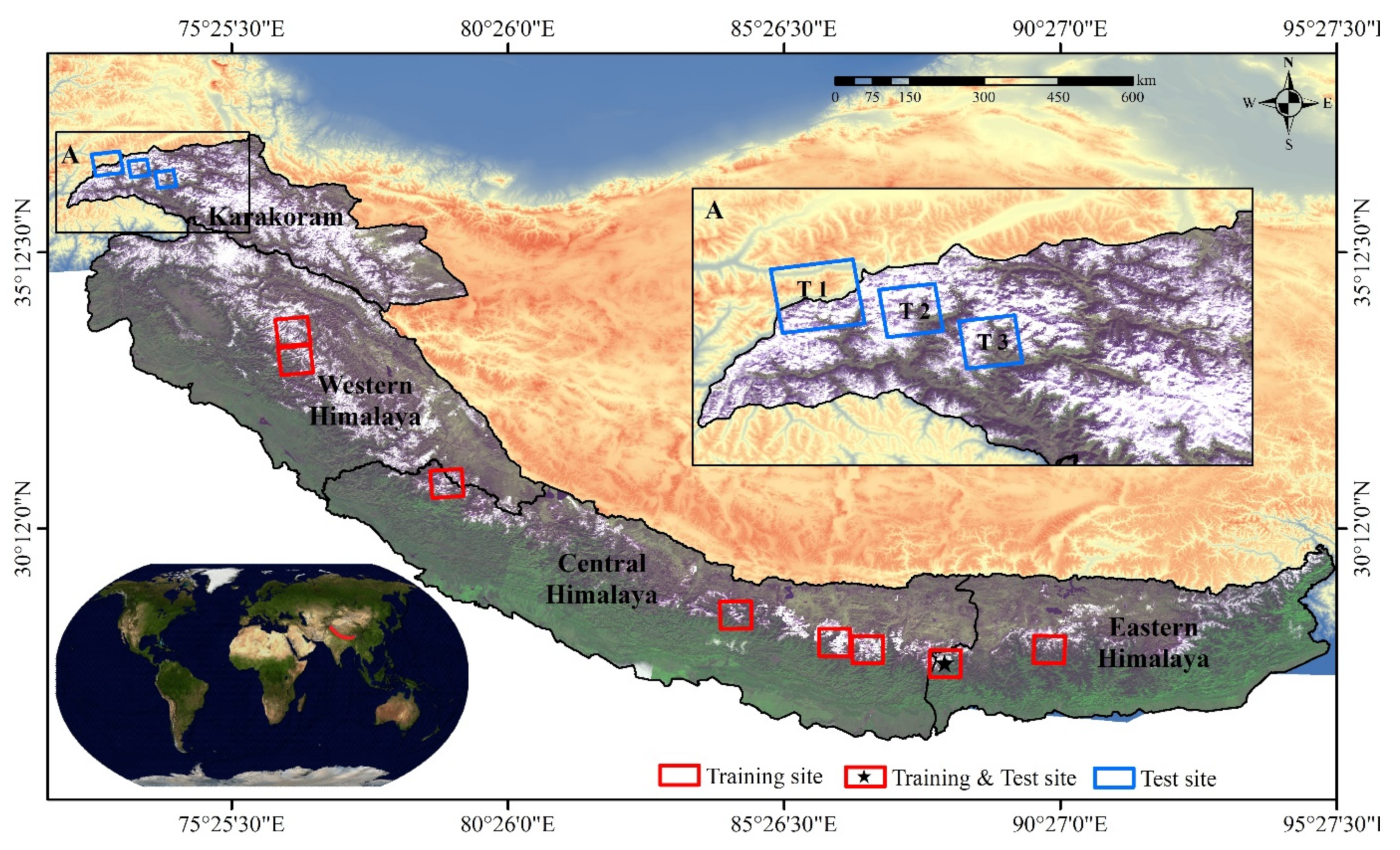
2.1. Study Site
2.2. Data Used
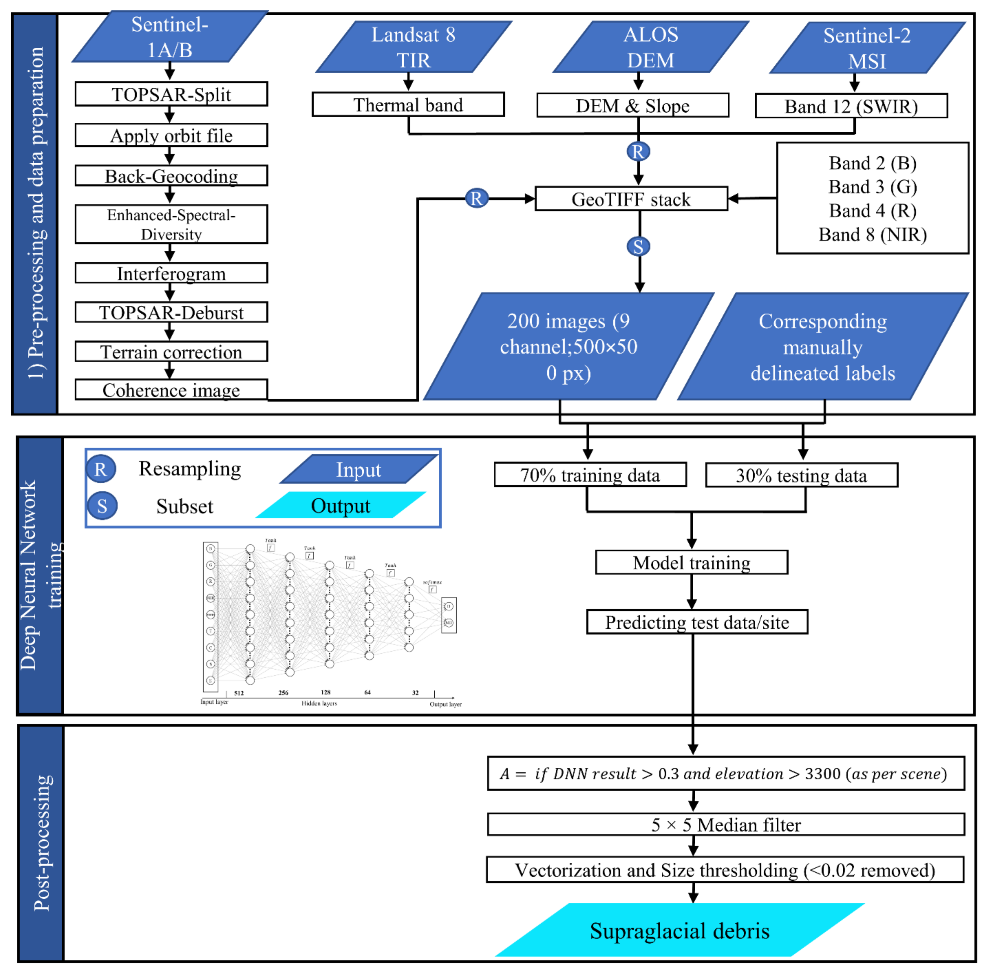
2.3. Pre-Processing and Data Preparation
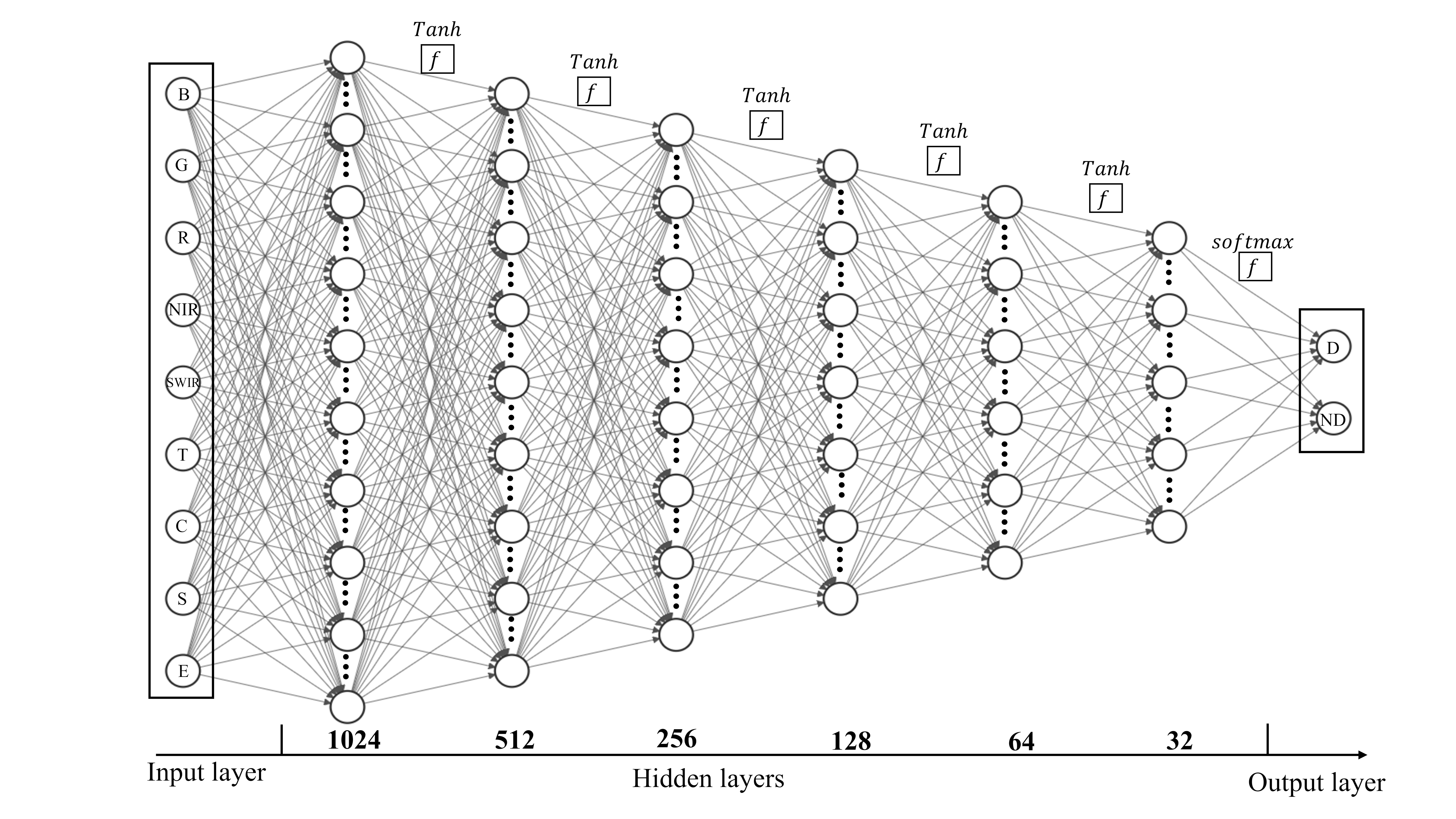
2.4. Deep Neural Network Architecture (SGDNet)
2.5. Post Processing
2.6. Accuracy Assessment
3. Results
3.1. Proposed Deep Artificial Neural Network (SGDNet)
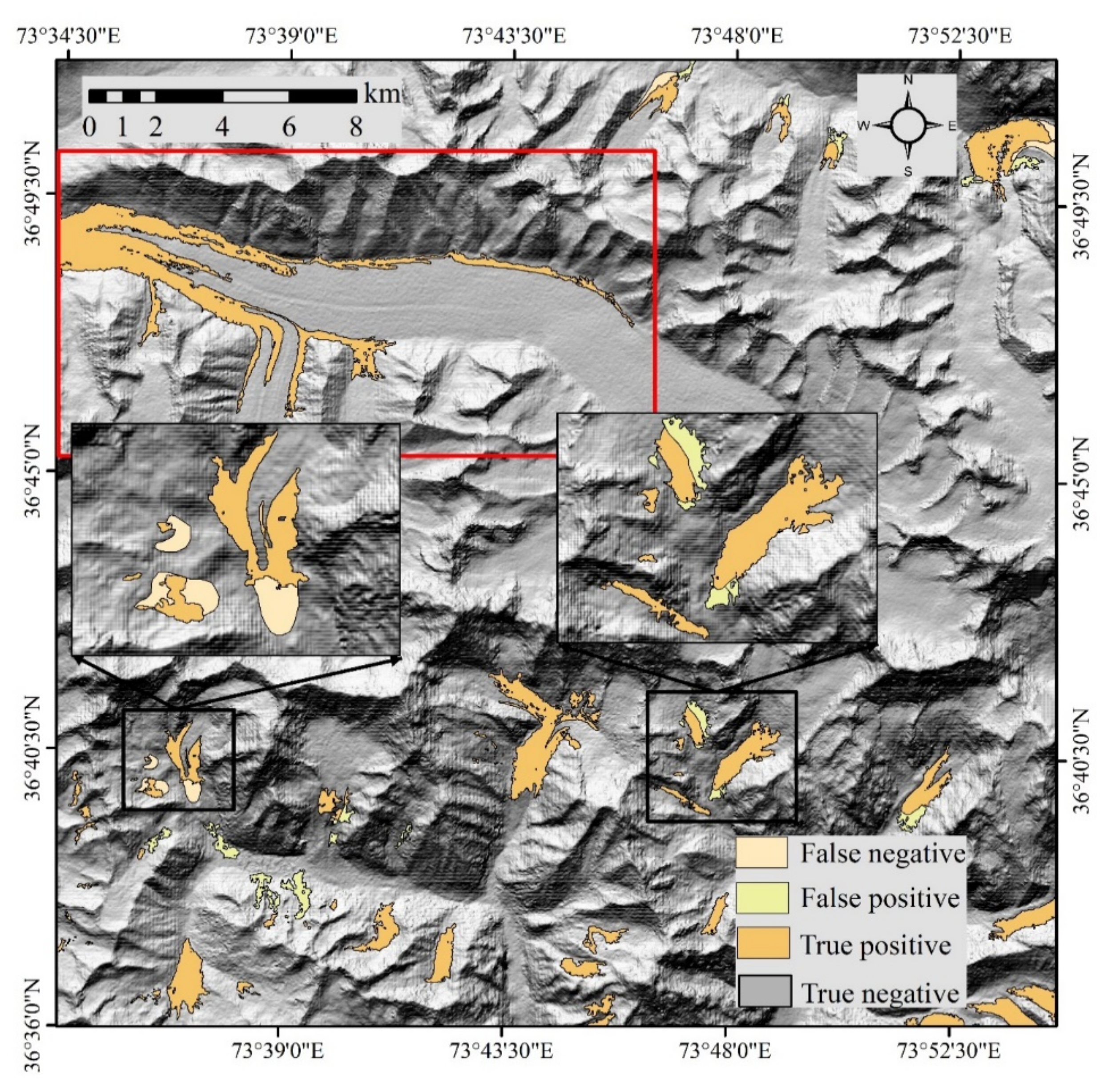
3.2. Test Site 1, 2, and 3
4. Discussion
4.1. Proposed DNN (SGDNet) for SGD Mapping
4.2. Classification Results and Comparison with Existing Methods
4.3. Limitations and Future Work
5. Conclusions
Supplementary Materials
Author Contributions
Funding
Data Availability Statement
Acknowledgments
Conflicts of Interest
References
- Maurer, J.M.; Schaefer, J.; Rupper, S.; Corley, A.J.S.A. Acceleration of ice loss across the Himalayas over the past 40 years. Sci. Adv. 2019, 5, eaav7266. [Google Scholar] [CrossRef] [PubMed] [Green Version]
- Immerzeel, W.W.; Lutz, A.; Andrade, M.; Bahl, A.; Biemans, H.; Bolch, T.; Hyde, S.; Brumby, S.; Davies, B.; Elmore, A. Importance and vulnerability of the world’s water towers. Nature 2020, 577, 364–369. [Google Scholar] [CrossRef] [PubMed]
- Radić, V.; Bliss, A.; Beedlow, A.C.; Hock, R.; Miles, E.; Cogley, J.G. Regional and global projections of twenty-first century glacier mass changes in response to climate scenarios from global climate models. Clim. Dyn. 2014, 42, 37–58. [Google Scholar] [CrossRef]
- Hock, R.; Bliss, A.; Marzeion, B.; Giesen, R.H.; Hirabayashi, Y.; Huss, M.; Radić, V.; Slangen, A.B. GlacierMIP–A model intercomparison of global-scale glacier mass-balance models and projections. J. Glaciol. 2019, 65, 453–467. [Google Scholar] [CrossRef] [Green Version]
- Zemp, M.; Huss, M.; Thibert, E.; Eckert, N.; McNabb, R.; Huber, J.; Barandun, M.; Machguth, H.; Nussbaumer, S.U.; Gärtner-Roer, I. Global glacier mass changes and their contributions to sea-level rise from 1961 to 2016. Nature 2019, 568, 382–386. [Google Scholar] [CrossRef]
- Huss, M.; Jouvet, G.; Farinotti, D.; Bauder, A. Future high-mountain hydrology: A new parameterization of glacier retreat. Hydrol. Earth Syst. Sci. 2010, 14, 815–829. [Google Scholar] [CrossRef] [Green Version]
- Cauvy-Fraunié, S.; Andino, P.; Espinosa, R.; Calvez, R.; Jacobsen, D.; Dangles, O. Ecological responses to experimental glacier-runoff reduction in alpine rivers. Nat. Commun. 2016, 7, 12025. [Google Scholar] [CrossRef] [Green Version]
- Cannone, N.; Diolaiuti, G.; Guglielmin, M.; Smiraglia, C. Accelerating climate change impacts on alpine glacier forefield ecosystems in the European Alps. Ecol. Appl. 2008, 18, 637–648. [Google Scholar] [CrossRef] [Green Version]
- Kumar, R.; Kumar, R.; Singh, A.; Singh, S.; Bhardwaj, A.; Kumari, A.; Sinha, R.K.; Gupta, A. Hydro-geochemical analysis of meltwater draining from Bilare Banga glacier, Western Himalaya. Acta Geophys. 2019, 67, 651–660. [Google Scholar] [CrossRef]
- Kumar, R.; Kumar, R.; Singh, S.; Singh, A.; Bhardwaj, A.; Chaudhary, H. Hydro-geochemical characteristics of glacial meltwater from Naradu Glacier catchment, Western Himalaya. Environ. Earth Sci. 2019, 78, 683. [Google Scholar] [CrossRef]
- Dyurgerov, M.B.; Meier, M.F. Twentieth century climate change: Evidence from small glaciers. Proc. Natl. Acad. Sci. USA 2000, 97, 1406–1411. [Google Scholar] [CrossRef] [Green Version]
- Marzeion, B.; Kaser, G.; Maussion, F.; Champollion, N. Limited influence of climate change mitigation on short-term glacier mass loss. Nat. Clim. Change 2018, 8, 305–308. [Google Scholar] [CrossRef]
- Patel, A.; Goswami, A.; Dharpure, J.K.; Thamban, M.; Kulkarni, A.V.; Sharma, P. Regional mass variations and its sensitivity to climate drivers over glaciers of Karakoram and Himalayas. GISci. Remote Sens. 2021, 58, 670–692. [Google Scholar] [CrossRef]
- Miles, E.; McCarthy, M.; Dehecq, A.; Kneib, M.; Fugger, S.; Pellicciotti, F. Health and sustainability of glaciers in High Mountain Asia. Nat. Commun. 2021, 12, 683. [Google Scholar] [CrossRef]
- Treichler, D.; Kääb, A.; Salzmann, N.; Xu, C.-Y. Recent glacier and lake changes in High Mountain Asia and their relation to precipitation changes. Cryosphere 2019, 13, 2977–3005. [Google Scholar] [CrossRef] [Green Version]
- Maurer, J.; Schaefer, J.; Russell, J.; Rupper, S.; Wangdi, N.; Putnam, A.; Young, N. Seismic observations, numerical modeling, and geomorphic analysis of a glacier lake outburst flood in the Himalayas. Sci. Adv. 2020, 6, eaba3645. [Google Scholar] [CrossRef]
- Kaushik, S.; Rafiq, M.; Joshi, P.; Singh, T. Examining the glacial lake dynamics in a warming climate and GLOF modelling in parts of Chandra basin, Himachal Pradesh, India. Sci. Total Environ. 2020, 714, 136455. [Google Scholar] [CrossRef] [PubMed]
- Brun, F.; Berthier, E.; Wagnon, P.; Kääb, A.; Treichler, D. A spatially resolved estimate of High Mountain Asia glacier mass balances from 2000 to 2016. Nat. Geosci. 2017, 10, 668–673. [Google Scholar] [CrossRef]
- Parkinson, C.L. Earth’s cryosphere: Current state and recent changes. Annu. Rev. Environ. Resour. 2006, 31, 33–60. [Google Scholar] [CrossRef] [Green Version]
- Williams, R.S., Jr.; Ferrigno, J.G. State of the Earth’s cryosphere at the beginning of the 21st century: Glaciers, global snow cover, floating ice, and permafrost and periglacial environments. Director 2012, 508, 344–6840. [Google Scholar]
- Khanal, S.; Lutz, A.F.; Kraaijenbrink, P.D.; van den Hurk, B.; Yao, T.; Immerzeel, W.W. Variable 21st century climate change response for rivers in High Mountain Asia at seasonal to decadal time scales. Water Resour. Res. 2021, 57, e2020WR029266. [Google Scholar] [CrossRef]
- Gardelle, J.; Berthier, E.; Arnaud, Y.; Kääb, A. Region-wide glacier mass balances over the Pamir-Karakoram-Himalaya during 1999–2011. Cryosphere 2013, 7, 1263–1286. [Google Scholar] [CrossRef] [Green Version]
- Huss, M.; Farinotti, D. Distributed ice thickness and volume of all glaciers around the globe. J. Geophys. Res. Earth Surf. 2012, 117, F04010. [Google Scholar] [CrossRef]
- Bhardwaj, A.; Joshi, P.K.; Singh, M.K.; Sam, L.; Gupta, R. Mapping debris-covered glaciers and identifying factors affecting the accuracy. Cold Reg. Sci. Technol. 2014, 106, 161–174. [Google Scholar] [CrossRef]
- Kaushik, S.; Joshi, P.; Singh, T. Development of glacier mapping in Indian Himalaya: A review of approaches. Int. J. Remote Sens. 2019, 40, 6607–6634. [Google Scholar] [CrossRef]
- Rounce, D.R.; Hock, R.; McNabb, R.; Millan, R.; Sommer, C.; Braun, M.; Malz, P.; Maussion, F.; Mouginot, J.; Seehaus, T. Distributed global debris thickness estimates reveal debris significantly impacts glacier mass balance. Geophys. Res. Lett. 2021, 48, e2020GL091311. [Google Scholar] [CrossRef]
- Scherler, D.; Bookhagen, B.; Strecker, M.R. Spatially variable response of Himalayan glaciers to climate change affected by debris cover. Nat. Geosci. 2011, 4, 156–159. [Google Scholar] [CrossRef]
- Sam, L.; Bhardwaj, A.; Kumar, R.; Buchroithner, M.F.; Martín-Torres, F.J. Heterogeneity in topographic control on velocities of Western Himalayan glaciers. Sci. Rep. 2018, 8, 12843. [Google Scholar] [CrossRef] [Green Version]
- Sam, L.; Bhardwaj, A.; Singh, S.; Kumar, R. Remote sensing flow velocity of debris-covered glaciers using Landsat 8 data. Prog. Phys. Geogr. 2016, 40, 305–321. [Google Scholar] [CrossRef]
- Kaushik, S.; Singh, T.; Bhardwaj, A.; Joshi, P. Long-term spatiotemporal variability in the glacier surface velocity of Eastern Himalayan glaciers, India. Earth Surf. Processes Landf. 2022. [Google Scholar] [CrossRef]
- King, O.; Dehecq, A.; Quincey, D.; Carrivick, J. Contrasting geometric and dynamic evolution of lake and land-terminating glaciers in the central Himalaya. Glob. Planet. Change 2018, 167, 46–60. [Google Scholar] [CrossRef]
- Shukla, A.; Arora, M.; Gupta, R. Synergistic approach for mapping debris-covered glaciers using optical–thermal remote sensing data with inputs from geomorphometric parameters. Remote Sens. Environ. 2010, 114, 1378–1387. [Google Scholar] [CrossRef]
- Hall, D.K.; Williams, R.S.J.; Bayr, K.J.J.E. Transactions American Geophysical Union. Glacier recession in Iceland and Austria. EoS Trans. Am. Geophys. Union 1992, 73, 129–141. [Google Scholar] [CrossRef]
- Kulkarni, A.V.; Karyakarte, Y. Observed changes in Himalayan glaciers. Curr. Sci. 2014, 106, 237–244. [Google Scholar]
- Paul, F.; Huggel, C.; Kääb, A. Combining satellite multispectral image data and a digital elevation model for mapping debris-covered glaciers. Remote Sens. Environ. 2004, 89, 510–518. [Google Scholar] [CrossRef]
- Robson, B.A.; Nuth, C.; Dahl, S.O.; Hölbling, D.; Strozzi, T.; Nielsen, P.R. Automated classification of debris-covered glaciers combining optical, SAR and topographic data in an object-based environment. Remote Sens. Environ. 2015, 170, 372–387. [Google Scholar] [CrossRef] [Green Version]
- Racoviteanu, A.E.; Williams, M.W.; Barry, R.G. Optical remote sensing of glacier characteristics: A review with focus on the Himalaya. Sensors 2008, 8, 3355–3383. [Google Scholar] [CrossRef] [Green Version]
- Alifu, H.; Vuillaume, J.-F.; Johnson, B.A.; Hirabayashi, Y. Machine-learning classification of debris-covered glaciers using a combination of Sentinel-1/-2 (SAR/optical), Landsat 8 (thermal) and digital elevation data. Geomorphology 2020, 369, 107365. [Google Scholar] [CrossRef]
- Holobâcă, I.-H.; Tielidze, L.G.; Ivan, K.; Elizbarashvili, M.; Alexe, M.; Germain, D.; Petrescu, S.H.; Pop, O.T.; Gaprindashvili, G. Multi-sensor remote sensing to map glacier debris cover in the Greater Caucasus, Georgia. J. Glaciol. 2021, 67, 685–696. [Google Scholar] [CrossRef]
- Kaushik, S.; Dharpure, J.K.; Joshi, P.; Ramanathan, A.; Singh, T. Climate change drives glacier retreat in Bhaga basin located in Himachal Pradesh, India. Geocarto Int. 2020, 35, 1179–1198. [Google Scholar] [CrossRef]
- Bhambri, R.; Bolch, T.; Chaujar, R. Mapping of debris-covered glaciers in the Garhwal Himalayas using ASTER DEMs and thermal data. Int. J. Remote Sens. 2011, 32, 8095–8119. [Google Scholar] [CrossRef] [Green Version]
- Xie, Z.; Haritashya, U.K.; Asari, V.K.; Young, B.W.; Bishop, M.P.; Kargel, J.S. GlacierNet: A deep-learning approach for debris-covered glacier mapping. IEEE Access 2020, 8, 83495–83510. [Google Scholar] [CrossRef]
- Lu, Y.; Zhang, Z.; Shangguan, D.; Yang, J. Novel Machine Learning Method Integrating Ensemble Learning and Deep Learning for Mapping Debris-Covered Glaciers. Remote Sens. 2021, 13, 2595. [Google Scholar] [CrossRef]
- Li, W.; Fu, H.; Yu, L.; Cracknell, A. Deep learning based oil palm tree detection and counting for high-resolution remote sensing images. Remote Sens. 2017, 9, 22. [Google Scholar] [CrossRef] [Green Version]
- Bishop, M.P.; Shroder, J.F.J.; Hickman, B.L. SPOT panchromatic imagery and neural networks for information extraction in a complex mountain environment. Geocarto Int. 1999, 14, 19–28. [Google Scholar] [CrossRef]
- Steiner, D.; Pauling, A.; Nussbaumer, S.U.; Nesje, A.; Luterbacher, J.; Wanner, H.; Zumbühl, H.J. Sensitivity of European glaciers to precipitation and temperature—Two case studies. Clim. Change 2008, 90, 413–441. [Google Scholar] [CrossRef] [Green Version]
- Robson, B.A.; Bolch, T.; MacDonell, S.; Hölbling, D.; Rastner, P.; Schaffer, N. Automated detection of rock glaciers using deep learning and object-based image analysis. Remote Sens. Environ. 2020, 250, 112033. [Google Scholar] [CrossRef]
- Dirscherl, M.; Dietz, A.J.; Kneisel, C.; Kuenzer, C. A Novel Method for Automated Supraglacial Lake Mapping in Antarctica Using Sentinel-1 SAR Imagery and Deep Learning. Remote Sens. 2021, 13, 197. [Google Scholar] [CrossRef]
- Nijhawan, R.; Das, J.; Balasubramanian, R. A hybrid CNN+ random forest approach to delineate debris covered glaciers using deep features. J. Indian Soc. Remote Sens. 2018, 46, 981–989. [Google Scholar] [CrossRef]
- Baumhoer, C.A.; Dietz, A.J.; Kneisel, C.; Kuenzer, C. Automated extraction of antarctic glacier and ice shelf fronts from sentinel-1 imagery using deep learning. Remote Sens. 2019, 11, 2529. [Google Scholar] [CrossRef] [Green Version]
- Marochov, M.; Stokes, C.R.; Carbonneau, P.E. Image Classification of Marine-Terminating Outlet Glaciers using Deep Learning Methods. Cryosphere 2020, 15, 5041–5059. [Google Scholar] [CrossRef]
- Bolibar, J.; Rabatel, A.; Gouttevin, I.; Galiez, C. A deep learning reconstruction of mass balance series for all glaciers in the French Alps: 1967–2015. Earth Syst. Sci. Data 2020, 12, 1973–1983. [Google Scholar] [CrossRef]
- Veh, G.; Korup, O.; Walz, A. Hazard from Himalayan glacier lake outburst floods. Proc. Natl. Acad. Sci. USA 2020, 117, 907–912. [Google Scholar] [CrossRef]
- Garg, P.K.; Shukla, A.; Jasrotia, A.S. On the strongly imbalanced state of glaciers in the Sikkim, eastern Himalaya, India. Sci. Total Environ. 2019, 691, 16–35. [Google Scholar] [CrossRef] [PubMed]
- Zheng, G.; Allen, S.K.; Bao, A.; Ballesteros-Cánovas, J.A.; Huss, M.; Zhang, G.; Li, J.; Yuan, Y.; Jiang, L.; Yu, T. Increasing risk of glacial lake outburst floods from future Third Pole deglaciation. Nat. Clim. Change 2021, 11, 411–417. [Google Scholar] [CrossRef]
- Farinotti, D.; Immerzeel, W.W.; de Kok, R.J.; Quincey, D.J.; Dehecq, A. Manifestations and mechanisms of the Karakoram glacier Anomaly. Nat. Geosci. 2020, 13, 8–16. [Google Scholar] [CrossRef] [PubMed]
- Quincey, D.; Braun, M.; Glasser, N.F.; Bishop, M.; Hewitt, K.; Luckman, A. Karakoram glacier surge dynamics. Geophys. Res. Lett. 2011, 28, 38. [Google Scholar] [CrossRef] [Green Version]
- Dehecq, A.; Gourmelen, N.; Gardner, A.S.; Brun, F.; Goldberg, D.; Nienow, P.W.; Berthier, E.; Vincent, C.; Wagnon, P.; Trouvé, E. Twenty-first century glacier slowdown driven by mass loss in High Mountain Asia. Nat. Geosci. 2019, 12, 22–27. [Google Scholar] [CrossRef]
- Nie, Y.; Sheng, Y.; Liu, Q.; Liu, L.; Liu, S.; Zhang, Y.; Song, C. A regional-scale assessment of Himalayan glacial lake changes using satellite observations from 1990 to 2015. Remote Sens. Environ. 2017, 189, 1–13. [Google Scholar] [CrossRef] [Green Version]
- Sharma, A.; Liu, X.; Yang, X.; Shi, D. A patch-based convolutional neural network for remote sensing image classification. Neural Netw. 2017, 95, 19–28. [Google Scholar] [CrossRef]
- Racoviteanu, A.; Williams, M.W. Decision tree and texture analysis for mapping debris-covered glaciers in the Kangchenjunga area, Eastern Himalaya. Remote Sens. 2012, 4, 3078–3109. [Google Scholar] [CrossRef] [Green Version]
- Lippl, S.; Vijay, S.; Braun, M. Automatic delineation of debris-covered glaciers using InSAR coherence derived from X-, C-and L-band radar data: A case study of Yazgyl Glacier. J. Glaciol. 2018, 64, 811–821. [Google Scholar] [CrossRef] [Green Version]
- Atwood, D.; Meyer, F.; Arendt, A. Using L-band SAR coherence to delineate glacier extent. Can. J. Remote Sens. 2010, 36, S186–S195. [Google Scholar] [CrossRef]
- Chowdhury, A.; Sharma, M.C.; De, S.K.; Debnath, M. Glacier Changes in the Chhombo Chhu Watershed of Tista basin between 1975 and 2018, Sikkim Himalaya, India. Earth Syst. Sci. Data 2021, 13, 2923–2944. [Google Scholar] [CrossRef]
- Basnett, S.; Kulkarni, A.V.; Bolch, T.J. The influence of debris cover and glacial lakes on the recession of glaciers in Sikkim Himalaya, India. J. Glaciol. 2013, 59, 1035–1046. [Google Scholar] [CrossRef] [Green Version]
- Bookhagen, B.; Burbank, D.W. Toward a complete Himalayan hydrological budget: Spatiotemporal distribution of snowmelt and rainfall and their impact on river discharge. J. Geophys. Res. Earth Surf. 2010, 115, 3546062. [Google Scholar] [CrossRef] [Green Version]
- Frey, H.; Paul, F.; Strozzi, T. Compilation of a glacier inventory for the western Himalayas from satellite data: Methods, challenges, and results. Remote Sens. Environ. 2012, 124, 832–843. [Google Scholar] [CrossRef] [Green Version]
- Pfeffer, W.T.; Arendt, A.A.; Bliss, A.; Bolch, T.; Cogley, J.G.; Gardner, A.S.; Hagen, J.-O.; Hock, R.; Kaser, G.; Kienholz, C. The Randolph Glacier Inventory: A globally complete inventory of glaciers. J. Glaciol. 2014, 60, 537–552. [Google Scholar] [CrossRef] [Green Version]
- Zlateski, A.; Jaroensri, R.; Sharma, P.; Durand, F. On the importance of label quality for semantic segmentation. In Proceedings the IEEE Conference on Computer Vision and Pattern Recognition, Salt Lake City, UT, USA, 18–22 June 2018; pp. 1479–1487. [Google Scholar]
- Kingma, D.P.; Ba, J. Adam: A method for stochastic optimization. arXiv 2014, arXiv:1412.6980. [Google Scholar]
- Chen, Y.; Lin, Z.; Zhao, X.; Wang, G.; Gu, Y. Deep learning-based classification of hyperspectral data. IEEE J. Sel. Top. Appl. Earth Obs. Remote Sens. 2014, 7, 2094–2107. [Google Scholar] [CrossRef]
- Herreid, S.; Pellicciotti, F. The state of rock debris covering Earth’s glaciers. Nat. Geosci. 2020, 13, 621–627. [Google Scholar] [CrossRef]
- Wang, Y.; Lv, H.; Deng, R.; Zhuang, S. A Comprehensive Survey of Optical Remote Sensing Image Segmentation Methods. Can. J. Remote Sens. 2020, 46, 501–531. [Google Scholar] [CrossRef]
- Yanlei, G.; Chao, T.; Jing, S.; Zhengrong, Z. High-resolution remote sensing image semantic segmentation based on semi-supervised full convolution network method. Acta Geod. Cartogr. Sin. 2020, 49, 499. [Google Scholar]


| Statistical Metric | Sikkim * | T1 | T2 | T3 |
|---|---|---|---|---|
| Accuracy | 0.99 | 0.99 | 0.98 | 0.99 |
| Recall | 0.81 | 0.88 | 0.82 | 0.96 |
| Precision | 0.99 | 0.88 | 0.86 | 0.91 |
| F-Score | 0.89 | 0.88 | 0.84 | 0.94 |
| False positive area (km2) | 0.2 | 3.16 | 8.22 | 3.56 |
| False negative area (km2) | 11.23 | 3.29 | 11.08 | 1.35 |
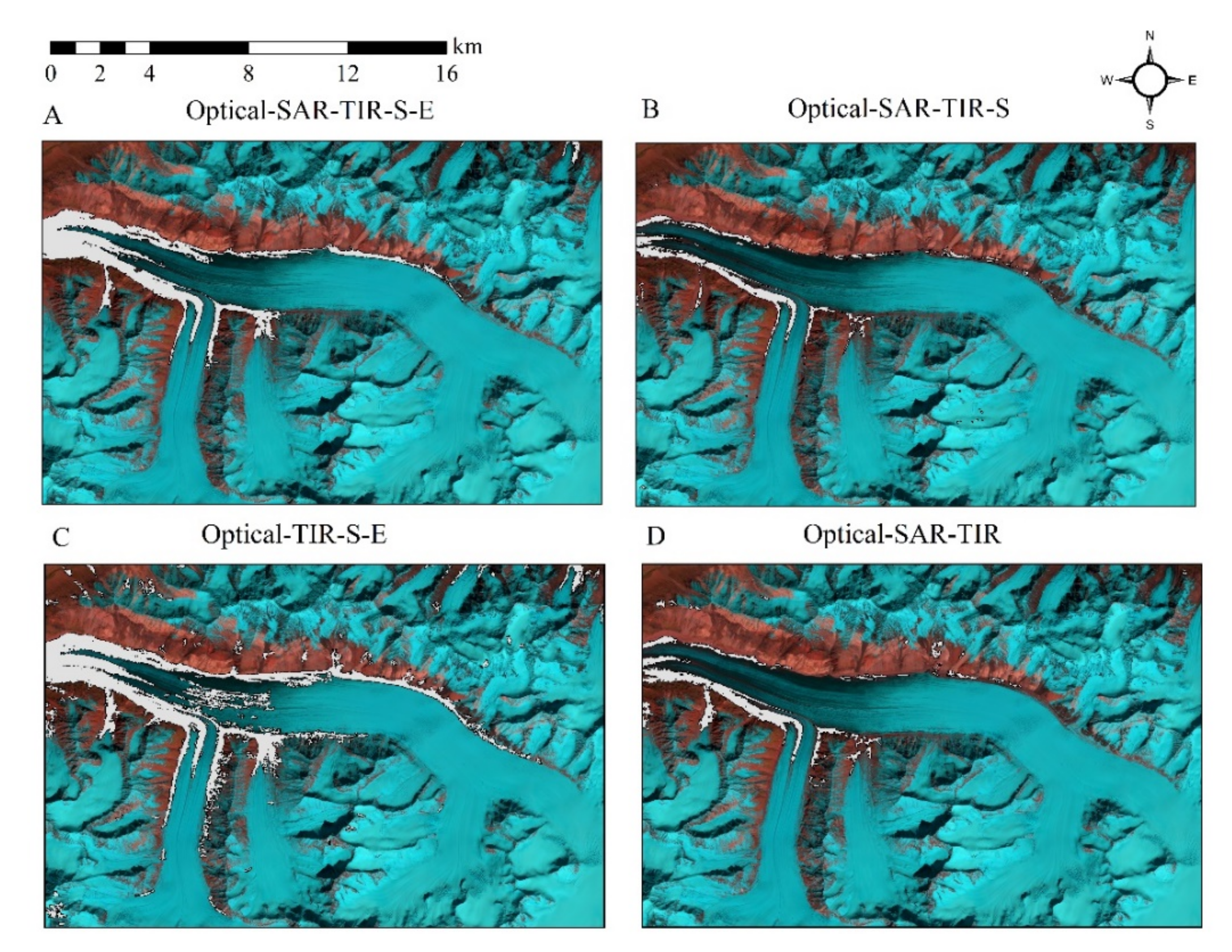
| Accuracy | Recall | Precision | F-Score | Dataset Used |
|---|---|---|---|---|
| 0.93 | 0.59 | 0.71 | 0.64 | Optical-SAR-TIR-S |
| 0.96 | 0.78 | 0.81 | 0.79 | Optical-TIR-S-E |
| 0.91 | 0.37 | 0.65 | 0.47 | Optical-SAR-TIR |
Publisher’s Note: MDPI stays neutral with regard to jurisdictional claims in published maps and institutional affiliations. |
© 2022 by the authors. Licensee MDPI, Basel, Switzerland. This article is an open access article distributed under the terms and conditions of the Creative Commons Attribution (CC BY) license (https://creativecommons.org/licenses/by/4.0/).
Share and Cite
Kaushik, S.; Singh, T.; Bhardwaj, A.; Joshi, P.K.; Dietz, A.J. Automated Delineation of Supraglacial Debris Cover Using Deep Learning and Multisource Remote Sensing Data. Remote Sens. 2022, 14, 1352. https://0-doi-org.brum.beds.ac.uk/10.3390/rs14061352
Kaushik S, Singh T, Bhardwaj A, Joshi PK, Dietz AJ. Automated Delineation of Supraglacial Debris Cover Using Deep Learning and Multisource Remote Sensing Data. Remote Sensing. 2022; 14(6):1352. https://0-doi-org.brum.beds.ac.uk/10.3390/rs14061352
Chicago/Turabian StyleKaushik, Saurabh, Tejpal Singh, Anshuman Bhardwaj, Pawan K. Joshi, and Andreas J. Dietz. 2022. "Automated Delineation of Supraglacial Debris Cover Using Deep Learning and Multisource Remote Sensing Data" Remote Sensing 14, no. 6: 1352. https://0-doi-org.brum.beds.ac.uk/10.3390/rs14061352