
Improved-UWB/LiDAR-SLAM Tightly Coupled Positioning System with NLOS Identification Using a LiDAR Point Cloud in GNSS-Denied Environments


Abstract
:1. Introduction
- In complex environments, such as large buildings or time-varying environments, where UWB signals are heavily affected by NLOS errors, the rich geometric features enable LiDAR-SLAM to provide accurate and robust pose estimation and mapping results. With the advanced LiDAR-SLAM algorithm LeGO-LOAM, we propose and implement UWB NLOS identification using the LiDAR point cloud algorithm. This method combines the position information of the UWB anchor with the environment map generated by LeGO-LOAM and distinguishes between LOS and NLOS measurements in real time by efficiently and accurately performing obstacle detection and NLOS identification toward the line-of-sight direction of the anchor to improve the UWB data quality. It has good universality as it does not need the tedious data collection work and training phase in the early stage, and it can cope with the interference of dynamic obstacles in the environment well. Experimental results show that this NLOS identification algorithm is reasonably effective without adding a large amount of computation.
- To suppress the error accumulation of LiDAR-SLAM while simultaneously obtaining the positioning results in the world coordinate system, we propose a novel improved-UWB/LiDAR-SLAM tightly coupled positioning system by using UWB LOS measurements identified by the LiDAR point cloud and the positioning results of LeGO-LOAM as the input to the integrated system. Considering that in addition to NLOS propagation, UWB measurements are affected by signal multipath effects, intensity attenuation and other factors, which are likely to cause large gross errors, we use a robust extended Kalman filter (REKF) for parameter solutions and effectively suppress the influence of abnormal measurements on the filtering results by reducing the weights of outliers. A dynamic positioning experiment demonstrates the accuracy and robustness of the proposed tightly coupled integrated method combining NLOS identification and REKF.
2. Methodology
2.1. System Overview
2.2. Spatiotemporal Synchronization of Sensors
- Considering that the indoor ground is mostly horizontal, the transformation relationship between the w-frame and b-frame is obtained by observing the front and rear points on the side of the mobile platform with a high-precision total station.
- Because the LiDAR sensor remains fixed after installation, the transformation relationship between the b-frame and l-frame needs to be calibrated only once. A feature-rich static scenario is selected, and the mobile platform is kept stationary. Multiple pairs of corresponding feature points are obtained by observing the sharp-shaped corner feature points in the scenario from two different positions using LiDAR and a high-precision total station. The point observed by the total station is transformed into in accordance with , and the corresponding feature point pairs in the b-frame and l-frame are obtained. Thus, the transformation relationship between the b-frame and l-frame is obtained by solving for the four parameters.
- The transformation relationship between the w-frame and l-frame is . Since the g-frame and are coincident at the initial time, . Accordingly, the UWB anchor coordinates in the g-frame and the lever-arm vector with the LiDAR center pointing to the UWB mobile tag in the l-frame can be obtained. In this paper, because the LiDAR center and the UWB mobile tag are on the same plumb line, therefore , where d is the distance between the LiDAR center and the UWB mobile tag.
2.3. Generation of LiDAR Point Cloud Map
- Segmentation: The point cloud obtained at time t is set to , where is a point in the point cloud . The point cloud is projected into a range image with a resolution of 1800 × 16. The ground point cloud () and nonground point cloud () are extracted from the LiDAR raw data by judging the vertical dimensional characteristic.
- Feature extraction: To extract features uniformly from all directions from ground points and segmentation points, the range image is equally divided into several subimages in the horizonal direction. The smoothness of each point is calculated and compared with the smoothness threshold to extract the edge features and planar features for registration.
- Odometry: The scan-to-scan constraint based on extracted features is built next. Since the ground remains essentially constant between consecutive frames, the variations in the vertical dimension can be estimated based on the planar features. The estimate of the vertical dimension is input as the initial value into the second optimization step to reduce the number of iterations, and the variations in the horizontal dimension are calculated to improve the computational efficiency.
- Mapping: The scan-to-map constraint is constructed by the Levenberg–Marquardt (L-M) method, and the final global map is obtained using a loop detection approach. More details of the LeGO-LOAM algorithm can be found in [32].
2.4. UWB NLOS Identification Using a LiDAR Point Cloud Map
- At the initial time, the g-frame coincides with the . In accordance with the transformation relationship between the w-frame and g-frame calculated in Section 2.2, the UWB mobile tag coordinate and anchor coordinates in the w-frame are transformed into the g-frame (i.e., ). The lever-arm vector between the UWB mobile tag and the LiDAR sensor in the l-frame and the UWB anchor coordinates in the g-frame are obtained.
- At time t, the LiDAR coordinate is used to deduce the UWB mobile tag coordinate in the g-frame in accordance with the lever-arm vector .
- K-dimensional trees (KD-trees) and voxel grids are commonly used for map representation and corresponding searches in SLAM systems [36,39]. Considering that KD-tree representation can find the association points through a nearest neighbor search or radius search, we convert the point cloud map generated in Section 2.3 into a KD-tree structure for subsequent obstacle detection.
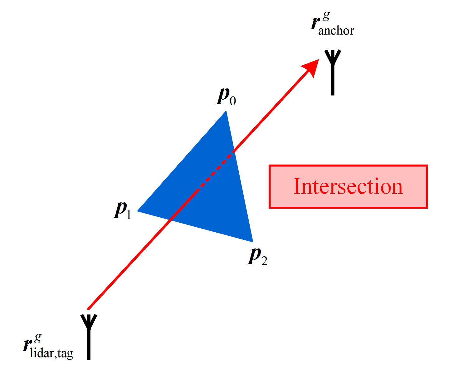
- Based on the UWB mobile tag coordinate and anchor j coordinate , the line-of-sight direction, i.e., the search direction for NLOS identification (e.g., the direction of the red dashed line in Figure 4), is determined. At the same time, the distance , vertical azimuth , and horizontal azimuth between the mobile tag and anchor j are calculated.Figure 4. NLOS identification using a LiDAR point cloud.
![Remotesensing 14 01380 g004]()
- The first NLOS identification is performed along the line of sight, centered on the UWB mobile tag position.
- Considering the general size of indoor objects and the LiDAR vertical angular resolution, the constructed KD-tree is used to search the point cloud in the neighborhood with a radius of 1 m. If the number of points in the neighborhood exceeds the given threshold (in this paper, ), it is considered that the line-of-sight direction may be blocked by obstacles.
- To prevent misjudgment (orange dashed block in Figure 4) and improve the accuracy of NLOS identification, based on the principle of collision detection, we traverse all points of the LiDAR point cloud in the neighborhood, take any three points to construct a triangle, and use Plücker coordinates to determine whether the line of sight intersects with the triangle in 3-D space. The Plücker coordinates represent a method of specifying directed lines in 3-D space using six-dimensional vectors. Taking any different points and to construct the Plücker coordinates l of line ab, we obtain:

- 8.
- If a triangle intersects with the line of sight, it is considered that the line-of-sight direction is blocked by obstacles, i.e., the status between the UWB mobile tag and anchor j is NLOS. This stops the detection and marks anchor j as an NLOS anchor. Otherwise, we consider that there is no obstacle occlusion at the current position and continue with the detection.
- 9.
- The search center point is moved to the next point in accordance with Equation (7), taking 2 m as the step size along the line of sight. Steps 6–8 are repeated to continue searching the point cloud for NLOS identification for anchor j.
- 10.
- When , the NLOS identification process for anchor j ends, and anchor j is marked as an LOS anchor.
- 11.
- Steps 4–10 are repeated to complete NLOS identification for all UWB anchors and distinguish between the LOS anchor set and the NLOS anchor set . The LOS anchor measurements will be used as input to the UWB module in the integrated positioning system.
2.5. Improved-UWB/LiDAR-SLAM Tightly Coupled Integrated Model
2.6. Innovation-Based Outlier-Resistant Robust EKF Algorithm
3. Experiments and Discussions
3.1. System Hardware
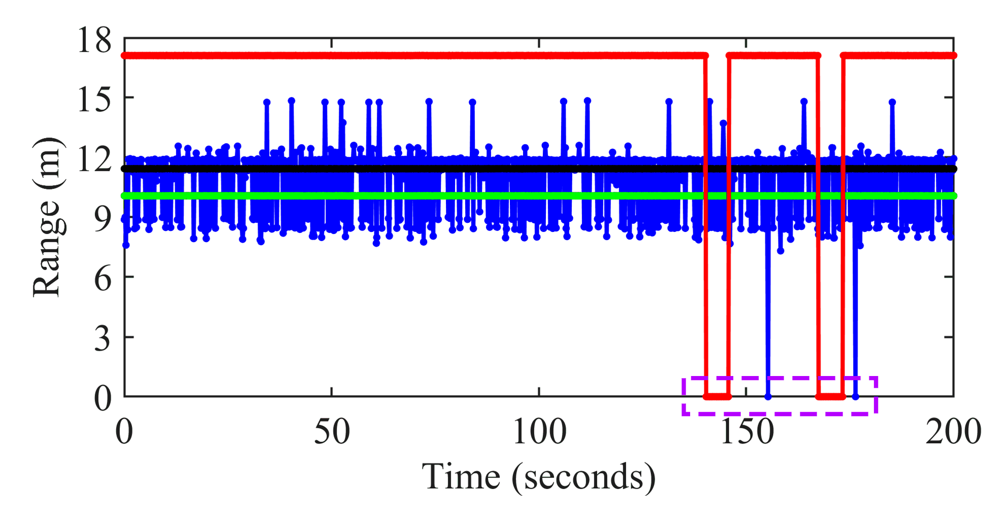
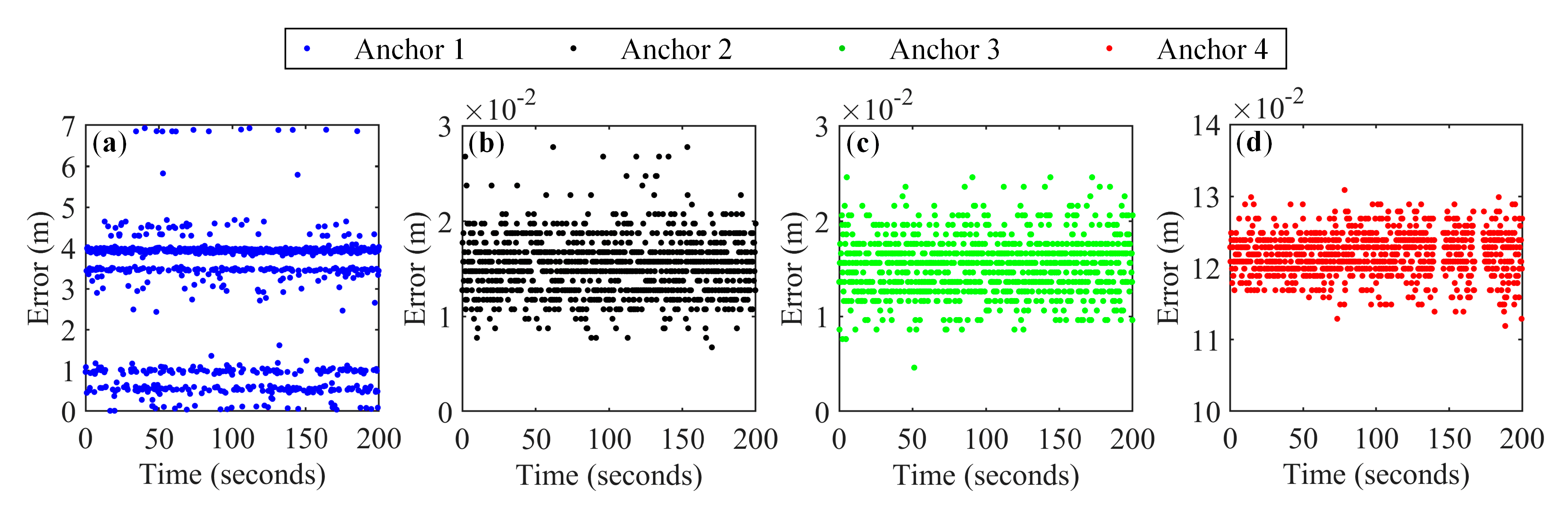
3.2. Evaluation of the UWB NLOS Identification Algorithm Using Static Data
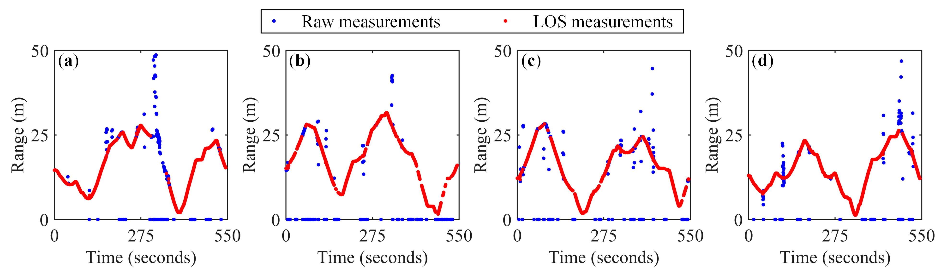
3.3. Evaluation of the UWB NLOS Identification Algorithm Using Dynamic Data
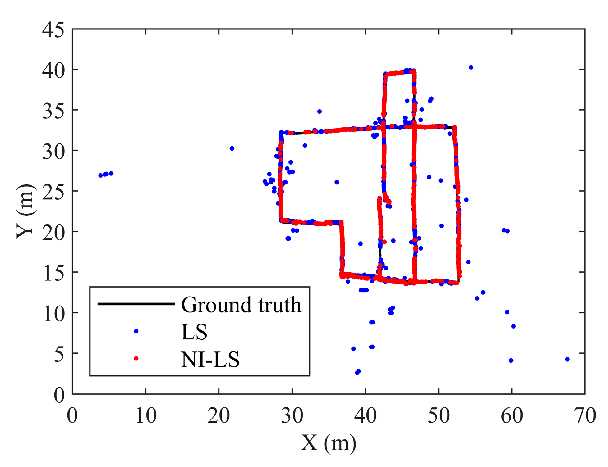
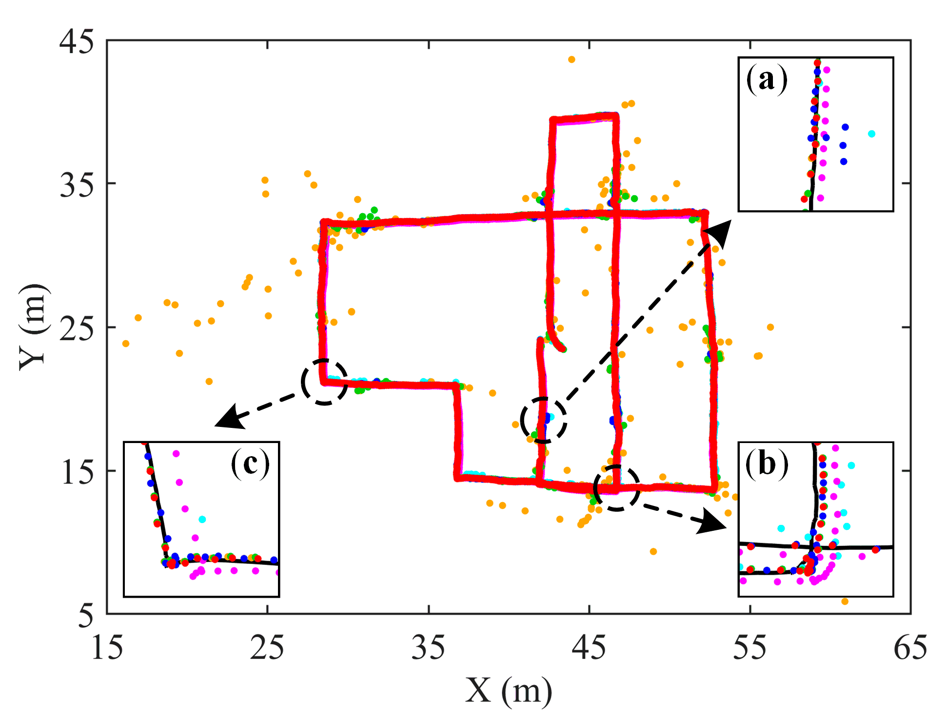
3.4. Evaluation of the Improved-UWB/LiDAR-SLAM Tightly Coupled Positioning Algorithm
- NI-LS;
- LeGO-LOAM without loop closure;
- UWB/LiDAR-SLAM tightly coupled algorithm with the EKF (UWB/LiDAR-SLAM tightly coupled + EKF, TC-EKF);
- UWB/LiDAR-SLAM tightly coupled algorithm with the REKF (UWB/LiDAR-SLAM tightly coupled + REKF, TC-REKF);
- Improved-UWB/LiDAR-SLAM tightly coupled algorithm with the EKF (NLOS identification + UWB/LiDAR-SLAM tightly coupled + EKF, NI-TC-EKF).
4. Conclusions
Author Contributions
Funding
Institutional Review Board Statement
Informed Consent Statement
Data Availability Statement
Conflicts of Interest
References
- Liu, T.; Yuan, Y.; Zhang, B.; Wang, N.; Tan, B.; Chen, Y. Multi-GNSS precise point positioning (MGPPP) using raw observations. J. Geod. 2017, 91, 253–268. [Google Scholar] [CrossRef]
- Zhou, F.; Dong, D.; Li, P.; Li, X.; Schuh, H. Influence of stochastic modeling for inter-system biases on multi-GNSS undifferenced and uncombined precise point positioning. GPS Solut. 2019, 23, 59. [Google Scholar] [CrossRef]
- Li, Z.; Chen, W.; Ruan, R.; Liu, X. Evaluation of PPP-RTK based on BDS-3/BDS-2/GPS observations: A case study in Europe. GPS Solut. 2020, 24, 38. [Google Scholar] [CrossRef]
- Yang, X. NLOS mitigation for UWB localization based on sparse pseudo-input Gaussian process. IEEE Sens. J. 2018, 18, 4311–4316. [Google Scholar] [CrossRef]
- Khodjaev, J.; Park, Y.; Saeed, M.A. Survey of NLOS identification and error mitigation problems in UWB-based positioning algorithms for dense environments. Ann. Telecommun. 2010, 65, 301–311. [Google Scholar] [CrossRef]
- Borras, J.; Hatrack, P.; Mandayam, N.B. Decision Theoretic Framework for NLOS Identification. In Proceedings of the 48th IEEE Vehicular Technology Conference, Ottawa, ON, Canada, 21 May 1998. [Google Scholar]
- Schroeder, J.; Galler, S.; Kyamakya, K.; Jobmann, K. NLOS detection algorithms for ultra-wideband localization. In Proceedings of the 2007 4th Workshop on Positioning, Navigation and Communication, Hannover, Germany, 22 March 2007. [Google Scholar]
- Maranò, S.; Gifford, W.M.; Wymeersch, H.; Win, M.Z. NLOS identification and mitigation for localization based on UWB experimental data. IEEE J. Sel. Area. Comm. 2010, 28, 1026–1035. [Google Scholar] [CrossRef] [Green Version]
- Wymeersch, H.; Maranò, S.; Gifford, W.M.; Win, M.Z. A machine learning approach to ranging error mitigation for UWB localization. IEEE Trans. Commun. 2012, 60, 1719–1728. [Google Scholar] [CrossRef] [Green Version]
- Savic, V.; Ferrer-Coll, J.; Ängskog, P.; Chilo, J.; Stenumgaard, P.; Larsson, E.G. Measurement analysis and channel modeling for TOA-based ranging in tunnels. IEEE Trans. Wirel. Commun. 2014, 14, 456–467. [Google Scholar] [CrossRef] [Green Version]
- Savic, V.; Larsson, E.G.; Ferrer-Coll, J.; Stenumgaard, P. Kernel methods for accurate UWB-based ranging with reduced complexity. IEEE Trans. Wirel. Commun. 2015, 15, 1783–1793. [Google Scholar] [CrossRef] [Green Version]
- Silva, B.; Hancke, G.P. IR-UWB-based non-line-of-sight identification in harsh environments: Principles and challenges. IEEE Trans. Ind. Inform. 2016, 12, 1188–1195. [Google Scholar] [CrossRef]
- Yu, K.; Wen, K.; Li, Y.; Zhang, S.; Zhang, K. A novel NLOS mitigation algorithm for UWB localization in harsh indoor environments. IEEE Trans. Veh. Technol. 2018, 68, 686–699. [Google Scholar] [CrossRef]
- Jiang, C.; Shen, J.; Chen, S.; Chen, Y.; Liu, D.; Bo, Y. UWB NLOS/LOS classification using deep learning method. IEEE Commun. Lett. 2020, 24, 2226–2230. [Google Scholar] [CrossRef]
- Jo, Y.H.; Lee, J.Y.; Ha, D.H.; Kang, S.H. Accuracy enhancement for UWB indoor positioning using ray tracing. In Proceedings of the IEEE/ION PLANS 2006, San Diego, CA, USA, 25–27 April 2006. [Google Scholar]
- Suski, W.; Banerjee, S.; Hoover, A. Using a map of measurement noise to improve UWB indoor position tracking. IEEE Trans. Instrum. Meas. 2013, 62, 2228–2236. [Google Scholar] [CrossRef]
- Zhu, X.; Yi, J.; Cheng, J.; He, L. Adapted error map based mobile robot UWB indoor positioning. IEEE Trans. Instrum. Meas. 2020, 69, 6336–6350. [Google Scholar] [CrossRef]
- Wang, C.; Xu, A.; Kuang, J.; Sui, X.; Hao, Y.; Niu, X. A High-Accuracy Indoor Localization System and Applications Based on Tightly Coupled UWB/INS/Floor Map Integration. IEEE Sens. J. 2021, 21, 18166–18177. [Google Scholar] [CrossRef]
- Wang, C.; Xu, A.; Sui, X.; Hao, Y.; Shi, Z.; Chen, Z. A Seamless Navigation System and Applications for Autonomous Vehicles Using a Tightly Coupled GNSS/UWB/INS/Map Integration Scheme. Remote Sens. 2022, 14, 27. [Google Scholar] [CrossRef]
- Ferreira, A.G.; Fernandes, D.; Branco, S.; Catarino, A.P.; Monteiro, J.L. Feature Selection for Real-Time NLOS Identification and Mitigation for Body-Mounted UWB Transceivers. IEEE Trans. Instrum. Meas. 2021, 70, 1–10. [Google Scholar] [CrossRef]
- Wen, K.; Yu, K.; Li, Y. NLOS identification and compensation for UWB ranging based on obstruction classification. In Proceedings of the 2017 25th European Signal Processing Conference (EUSIPCO), Kos, Greece, 28 August–2 September 2017. [Google Scholar]
- Wen, C.; Tan, J.; Li, F.; Wu, C.; Lin, Y.; Wang, Z.; Wang, C. Cooperative indoor 3D mapping and modeling using LiDAR data. Inf. Sci. 2021, 574, 192–209. [Google Scholar] [CrossRef]
- Wang, Q.; Tan, Y.; Mei, Z. Computational methods of acquisition and processing of 3D point cloud data for construction applications. Arch. Comput. Methods Eng. 2020, 27, 479–499. [Google Scholar] [CrossRef]
- Li, K.; Li, M.; Hanebeck, U.D. Towards high-performance solid-state-lidar-inertial odometry and mapping. IEEE Robot. Autom. Lett. 2021, 6, 5167–5174. [Google Scholar] [CrossRef]
- Magnusson, M.; Lilienthal, A.; Duckett, T. Scan registration for autonomous mining vehicles using 3D-NDT. J. Field Robot. 2007, 24, 803–827. [Google Scholar] [CrossRef] [Green Version]
- Biber, P.; Strasser, W. The normal distributions transform: A new approach to laser scan matching. In Proceedings of the 2003 IEEE/RSJ International Conference on Intelligent Robots and Systems (IROS 2003), Las Vegas, NV, USA, 27–31 October 2003. [Google Scholar]
- Landry, D.; Pomerleau, F.; Giguere, P. CELLO-3D: Estimating the Covariance of ICP in the Real World. In Proceedings of the 2019 International Conference on Robotics and Automation (ICRA), Montreal, QC, Canada, 20–24 May 2019. [Google Scholar]
- Brossard, M.; Bonnabel, S.; Barrau, A. A new approach to 3D ICP covariance estimation. IEEE Robot. Autom. Lett. 2020, 5, 744–751. [Google Scholar] [CrossRef] [Green Version]
- Zhang, J.; Singh, S. Low-drift and real-time lidar odometry and mapping. Auton. Robot. 2017, 41, 401–416. [Google Scholar] [CrossRef]
- Geiger, A.; Lenz, P.; Urtasun, R. Are we ready for autonomous driving? The kitti vision benchmark suite. In Proceedings of the 2012 IEEE conference on computer vision and pattern recognition, Providence, RI, USA, 16–21 June 2012. [Google Scholar]
- Li, S.; Li, G.; Wang, L.; Qin, Y. SLAM integrated mobile mapping system in complex urban environments. ISPRS J. Photogramm. Remote Sens. 2020, 166, 316–332. [Google Scholar] [CrossRef]
- Shan, T.; Englot, B. Lego-loam: Lightweight and ground-optimized lidar odometry and mapping on variable terrain. In Proceedings of the 2018 IEEE/RSJ International Conference on Intelligent Robots and Systems (IROS), Madrid, Spain, 1–5 October 2018. [Google Scholar]
- Kaess, M.; Johannsson, H.; Roberts, R.; Ila, V.; Leonard, J.J.; Dellaert, F. iSAM2: Incremental smoothing and mapping using the Bayes tree. Int. J. Robot. Res. 2012, 31, 216–235. [Google Scholar] [CrossRef]
- He, G.; Yuan, X.; Zhuang, Y.; Hu, H. An integrated GNSS/LiDAR-SLAM pose estimation framework for large-scale map building in partially GNSS-denied environments. IEEE Trans. Instrum. Meas. 2020, 70, 1–9. [Google Scholar] [CrossRef]
- Wen, W.; Zhang, G.; Hsu, L.T. GNSS NLOS exclusion based on dynamic object detection using LiDAR point cloud. IEEE Trans. Intell. Transp. 2019, 22, 853–862. [Google Scholar] [CrossRef]
- Wen, W. 3D LiDAR Aided GNSS Positioning and Its Application in Sensor Fusion for Autonomous Vehicles in Urban Canyons. Ph.D. Thesis, Hong Kong Polytechnic University, Hong Kong, China, July 2020. [Google Scholar]
- Li, T.; Pei, L.; Xiang, Y.; Wu, Q.; Xia, S.; Tao, L.; Guan, X.; Yu, W. P3-LOAM: PPP/LiDAR Loosely Coupled SLAM with Accurate Covariance Estimation and Robust RAIM in Urban Canyon Environment. IEEE Sens. J. 2020, 21, 6660–6671. [Google Scholar] [CrossRef]
- Chang, L.; Niu, X.; Liu, T. GNSS/IMU/ODO/LiDAR-SLAM Integrated Navigation System Using IMU/ODO Pre-Integration. Sensors 2020, 20, 4702. [Google Scholar] [CrossRef]
- Yokozuka, M.; Koide, K.; Oishi, S.; Banno, A. LiTAMIN: LiDAR-based Tracking and Mapping by Stabilized ICP for Geometry Approximation with Normal Distributions. In Proceedings of the 2020 IEEE/RSJ International Conference on Intelligent Robots and Systems (IROS), Las Vegas, CA, USA, 24 October–24 January 2021. [Google Scholar]
- Wen, W.; Kan, Y.C.; Hsu, L.T. Performance comparison of GNSS/INS integrations based on EKF and factor graph optimization. In Proceedings of the 32nd International Technical Meeting of the Satellite Division of The Institute of Navigation (ION GNSS+ 2019), Miami, FL, USA, 16–20 September 2019. [Google Scholar]
- Li, T.; Zhang, H.; Gao, Z.; Chen, Q.; Niu, X. High-accuracy positioning in urban environments using single-frequency multi-GNSS RTK/MEMS-IMU integration. Remote Sens. 2018, 10, 205. [Google Scholar] [CrossRef] [Green Version]
- Chiang, K.W.; Tsai, G.J.; Chang, H.W.; Joly, C.; El-Sheimy, N. Seamless navigation and mapping using an INS/GNSS/grid-based SLAM semi-tightly coupled integration scheme. Inform. Fusion 2019, 50, 181–196. [Google Scholar] [CrossRef]
- Liu, T.; Niu, X.; Kuang, J.; Cao, S.; Zhang, L.; Chen, X. Doppler shift mitigation in acoustic positioning based on pedestrian dead reckoning for smartphone. IEEE Trans. Instrum. Meas. 2020, 70, 1–11. [Google Scholar] [CrossRef]
- Chiang, K.W.; Tsai, G.J.; Li, Y.H.; Li, Y.; El-Sheimy, N. Navigation engine design for automated driving using INS/GNSS/3D LiDAR-SLAM and integrity assessment. Remote Sens. 2020, 12, 1564. [Google Scholar] [CrossRef]
- Yang, Y.; Song, L.; Xu, T. Robust estimator for correlated observations based on bifactor equivalent weights. J. Geod. 2002, 76, 353–358. [Google Scholar] [CrossRef]


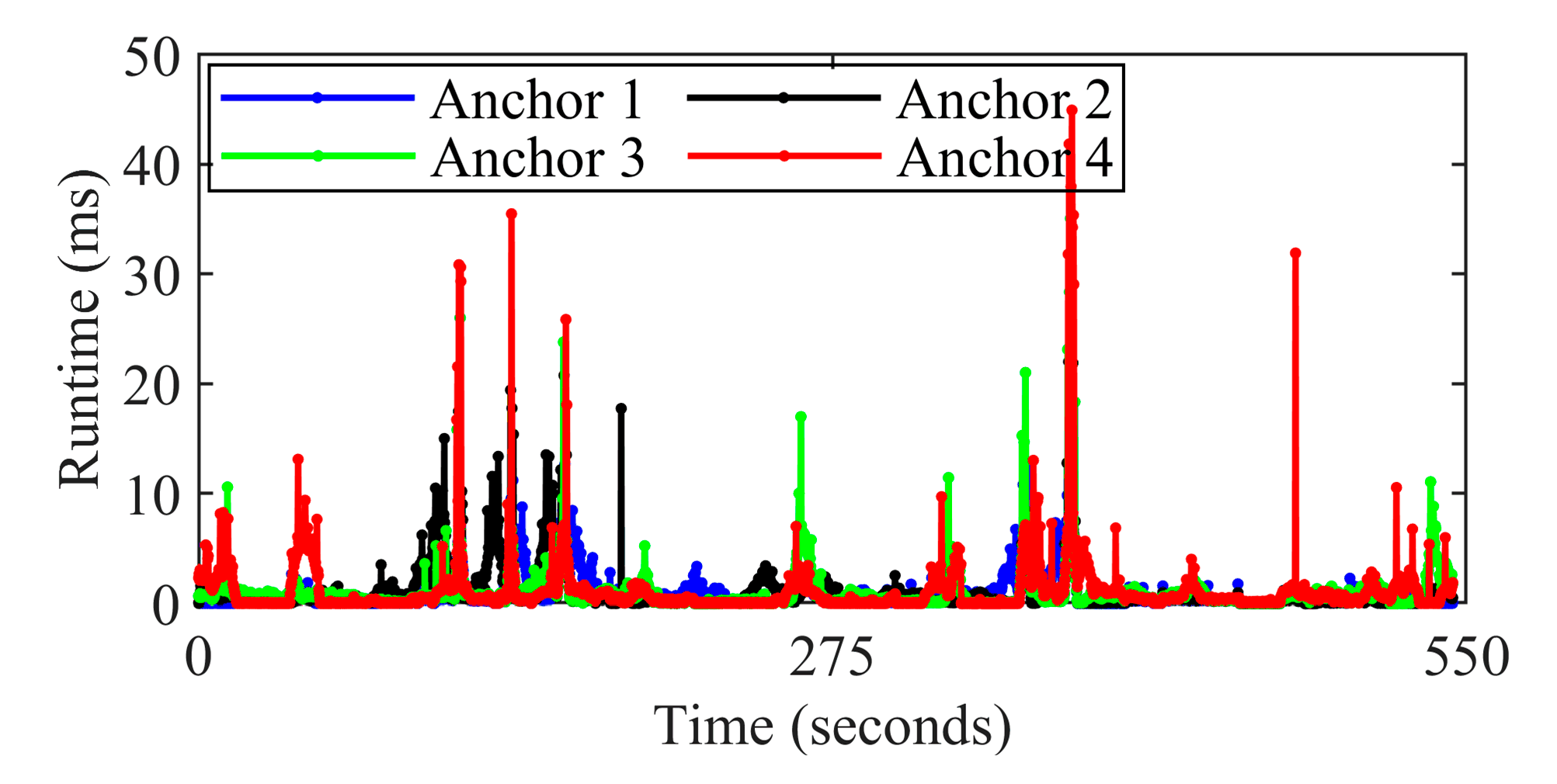
| Parameter | Anchor 1 | Anchor 2 | Anchor 3 | Anchor 4 |
|---|---|---|---|---|
| Distance (m) | 7.908 | 11.438 | 10.079 | 17.011 |
| Theoretical search times | 5 | 7 | 6 | 10 |
| Actual search times | 4 | 7 | 6 | 8 |
| Search time (ms) | 0.634 | 0.404 | 0.034 | 0.506 |
| Anchor 1 | Anchor 2 | Anchor 3 | Anchor 4 | ||
|---|---|---|---|---|---|
| Raw Measurements | RMSE (m) | 2.210 | 1.831 | 1.612 | 1.075 |
| MAX (m) | 37.105 | 30.562 | 51.658 | 28.330 | |
| LOS Measurements | RMSE (m) | 0.050 | 0.098 | 0.100 | 0.097 |
| MAX (m) | 0.902 | 0.629 | 0.879 | 0.704 | |
| LS | NI-LS | ||
|---|---|---|---|
| MAE (m) | X | 0.676 | 0.253 |
| Y | 0.691 | 0.307 | |
| Plane | 0.851 | 0.351 | |
| RMSE (m) | X | 2.226 | 0.079 |
| Y | 1.617 | 0.120 | |
| Plane | 2.752 | 0.144 | |
| Std (m) | X | 2.190 | 0.195 |
| Y | 1.560 | 0.226 | |
| Plane | 2.658 | 0.240 | |
| Max (m) | X | 30.006 | 0.590 |
| Y | 20.685 | 0.787 | |
| Plane | 30.483 | 0.826 | |
| Availability | 100% | 54.34% | |
| NI-LS | LeGO-LOAM | TC-EKF | TC-REKF | NI-TC-EKF | NI-TC-REKF | ||
|---|---|---|---|---|---|---|---|
| MAE (m) | X | 0.253 | 0.290 | 0.572 | 0.253 | 0.234 | 0.228 |
| Y | 0.307 | 0.265 | 0.550 | 0.253 | 0.236 | 0.230 | |
| Plane | 0.351 | 0.335 | 0.692 | 0.318 | 0.293 | 0.286 | |
| RMSE (m) | X | 0.079 | 0.087 | 1.210 | 0.105 | 0.072 | 0.066 |
| Y | 0.120 | 0.076 | 1.178 | 0.100 | 0.073 | 0.067 | |
| Plane | 0.144 | 0.115 | 1.688 | 0.145 | 0.103 | 0.094 | |
| Std (m) | X | 0.195 | 0.207 | 1.190 | 0.206 | 0.185 | 0.181 |
| Y | 0.226 | 0.197 | 1.165 | 0.204 | 0.186 | 0.182 | |
| Plane | 0.240 | 0.224 | 1.633 | 0.240 | 0.215 | 0.210 | |
| Max (m) | X | 0.590 | 0.372 | 12.801 | 1.167 | 0.394 | 0.317 |
| Y | 0.787 | 0.462 | 19.765 | 0.968 | 0.613 | 0.557 | |
| Plane | 0.826 | 0.482 | 21.965 | 1.169 | 0.621 | 0.566 | |
| Scale | Global | Local | Global | Global | Global | Global | |
| LiDAR-SLAM | NI | Tightly Coupled | Total | |
|---|---|---|---|---|
| Average (ms) | 560.849 | 41.099 | 0.017 | 602.657 |
| Max (ms) | 1072.22 | 160.754 | 0.124 | 1106.812 |
Publisher’s Note: MDPI stays neutral with regard to jurisdictional claims in published maps and institutional affiliations. |
© 2022 by the authors. Licensee MDPI, Basel, Switzerland. This article is an open access article distributed under the terms and conditions of the Creative Commons Attribution (CC BY) license (https://creativecommons.org/licenses/by/4.0/).
Share and Cite
Chen, Z.; Xu, A.; Sui, X.; Wang, C.; Wang, S.; Gao, J.; Shi, Z. Improved-UWB/LiDAR-SLAM Tightly Coupled Positioning System with NLOS Identification Using a LiDAR Point Cloud in GNSS-Denied Environments. Remote Sens. 2022, 14, 1380. https://0-doi-org.brum.beds.ac.uk/10.3390/rs14061380
Chen Z, Xu A, Sui X, Wang C, Wang S, Gao J, Shi Z. Improved-UWB/LiDAR-SLAM Tightly Coupled Positioning System with NLOS Identification Using a LiDAR Point Cloud in GNSS-Denied Environments. Remote Sensing. 2022; 14(6):1380. https://0-doi-org.brum.beds.ac.uk/10.3390/rs14061380
Chicago/Turabian StyleChen, Zhijian, Aigong Xu, Xin Sui, Changqiang Wang, Siyu Wang, Jiaxin Gao, and Zhengxu Shi. 2022. "Improved-UWB/LiDAR-SLAM Tightly Coupled Positioning System with NLOS Identification Using a LiDAR Point Cloud in GNSS-Denied Environments" Remote Sensing 14, no. 6: 1380. https://0-doi-org.brum.beds.ac.uk/10.3390/rs14061380