High-Precision Registration of Lunar Global Mapping Products Based on Spherical Triangular Mesh

Abstract

Lunar global mapping products provide a solid data foundation for lunar scientific research and exploration. As the widespread geometric inconsistencies among multi-source mapping products seriously affect the synergistic use of the products, high-precision registration of multiple lunar global products is critical, and it is highly challenging due to large coverage and complex local geometric inconsistencies. In this research, we propose a spherical triangular-mesh-based method for high-precision registration of lunar global mapping products, which involves four steps: data preprocessing, feature point extraction and matching, spherical Delaunay triangulation, and geometric correction with spherical barycentric coordinates. This global registration method avoids map projection distortions by using spherical coordinates directly, and achieves high precision by confining the geometric models to spherical triangular facets. Experiments are conducted using two groups of different types of mapping products to verify the proposed method quantitatively and qualitatively. The results show that the geometric inconsistencies are reduced from hundreds of pixels to sub-pixel level globally after the registration, demonstrating the effectiveness of the proposed method.

1. Introduction

Since the late 1950s, over a hundred lunar exploration missions have been carried out, from which massive data have been acquired by multiple sensors, such as cameras, spectrometers, laser altimeters, etc. The multi-source data and derived mapping products have greatly contributed to studies of the topography, geomorphology, mineralogy, and geologic evolution of the Moon. Particularly, various types of lunar global mapping products, which are essential for lunar global analyses, have been produced based on orbital data and photogrammetry and remote sensing technologies. For example, the U.S. Clementine mission acquired topographic data and multispectral imagery covering almost the entire Moon for the first time, from which lunar basemaps were produced [1,2,3]. These maps were later spatially registered to the Unified Lunar Control Network 2005 (ULCN2005) [4,5]. Based on the images obtained by the Wide-Angle Camera onboard the Lunar Reconnaissance Orbiter, a digital elevation model (DEM) covering the region between 79°N and 79°S and a global digital orthophoto mosaic (100 m/pixel) were produced [6,7,8]. Haruyama et al. [9] used data acquired from the SELENE Terrain Camera (TC) and Multi-band Imager (MI) from the JAXA SELENE/Kaguya mission to produce five lunar mosaic mapping products, namely TCOrtho_MAP, DTM_MAP, TC_Morning_MAP, and SLDEM. In addition, 59 m/pixel of multispectral mosaic products covering the region between 50°N and 50°S were created from the topographically corrected MI reflectance data [10,11]. Li et al. used Chang’E-1 (CE-1) three line-array image data and laser altimeter data to produce a lunar global digital topographic product (CE1TMap2009), including the 120 m/pixel digital orthophoto map (DOM) CE1_TMap_GDOM_120m, 500 m/pixel DEM CE1_TMap_GDEM_500m [12], and 3000 m/pixel DEM CE1_TMap_GDEM_3000m [13]. A new global lunar topographic product CE2TMap2015 (including DOM and DEM) was produced with different resolutions of 7 m, 20 m, and 50 m based on Chang’E-2 (CE-2) stereo images [14].

Based on lunar global mapping products from multiple sources, the advantages of different mapping products can be combined and fully utilized to provide a solid data foundation for lunar scientific research and exploration. However, varying degrees of geometric inconsistencies among lunar global mapping products from multiple sources widely exist [13,15,16]. This is due to the uncertainties in positions and attitudes of the different sensors onboard different orbiters or the same sensor at different times, and the differences in data processing and map production methods [17]. Geometric inconsistency seriously restricts the comparative study and synergistic use of lunar global mapping products; therefore, it is a prerequisite to accurately register these mapping products to the same reference before further exploitation [18]. Unlike local products, global products cover a wide range, and the map projection of a global product can have different distortions in different regions, which brings difficulties for global registration. Moreover, transformation models of traditional registration methods usually fail because global mapping products typically exhibit varying degrees of geometric inconsistencies in different local regions. Hence, it is challenging to register lunar global mapping products with high precision.

Kirk et al. [18] elucidated the significance of unifying the current lunar data, and presented the processing principles of how to register datasets to a common reference frame or to each other. Many studies have been performed for lunar local data registration. For example, Wu et al. [19] proposed a multi-feature-based surface matching method for the co-registration of multi-source lunar DEMs to produce high-precision lunar topographic models; For the co-registration between lunar orbital imagery and reference DEM, a pixel-based matching method considering both geometric and photometric information was developed by Xin et al. [20]. However, no result about lunar global mapping product registration has been reported as far as we know.

In the field of remote sensing, image registration has been extensively studied over the past few decades. Registration methods can be broadly divided into area-based and feature-based methods [21]. Compared with area-based algorithms, feature-based methods have the advantage of reducing computational cost, especially in the case of complex deformation [22]. Therefore, in this paper, we adopt feature-based methods to solve the lunar global mapping product registration problem. Feature detection and matching, transformation model establishment, image resampling, and registration accuracy assessment are the basic steps of feature-based methods. The first two steps play the most important role in the accuracy of image registration. During the past decades, most of the research has focused on feature detection and matching. The traditional local invariant features, such as scale-invariant feature transform (SIFT) [23], affine-SIFT (ASIFT) [24], speeded-up robust feature (SURF) [25], and so on have been widely used for the matching of remote sensing images. For multimodal remote sensing image registration, the most direct strategy achieves feature detection and description by directly modifying off-the-shelf methods, such as uniform robust SIFT (UR-SIFT) [26], scale restrict (SR-SIFT) [27], uniform nonlinear diffusion-based Harris (UND-Harris) [28], and so on. A growing number of studies are focusing on designing valid descriptors to construct more reliable feature matches so that transformation parameters can be estimated correctly, such as multiscale self-similarities (MSS) [29], distinctive order-based self-similarity descriptor (DOBSS) [30], rank-based local self-similarity (RLSS) [31], histogram of orientated phase congruency (HOPC) [32], channel feature of oriented gradient (CFOG) [33], guided local outlier factor (GLOF) [34], and advanced neighborhood topology consensus (ANTC) [35]. Deep-learning-based feature extraction methods have been developed recently, e.g., Li et al. [36] introduced a multi-task feature extraction network and self-supervised feature points. With feature points obtained, a transformation model such as affine [37], polynomial [38,39], projective [40], and so on can be estimated. The transformation model used in image registration can either be a global transformation or a local transformation. Most of the existing image registration research adopts the global transformation model [41,42], which usually ignores the local geometric deformation between images. Especially for images with wide coverage, large terrain variation, or complicated geometrical inconsistency, local geometric deformation cannot be effectively corrected by a global transformation model. In this case, researchers have studied the problem of complex local deformation and proposed some local transformation models to improve the accuracy of registration, e.g., piecewise linear model (PWLM) [43,44,45,46], local weighted mean method [47], thin plate spline [48,49,50], multiquadric functions [51], and as-projective-as-possible algorithm [52]. A few works on complex local registration in the remote sensing field have been reported, among which a triangular irregular network (TIN)-based method is most commonly used [53,54,55,56,57,58,59]. It first triangulates the image into 2D triangular facets using the Delaunay triangulation method [60] based on a control point set (the control points and their correspondences are given), and then the local transformation model within every triangular facet is estimated and applied for precise registration. The local transformation model adopted in this method is usually a 2D affine transformation model.

In this work, we propose a spherical triangular-mesh-based registration method as a solution to high-precision registration of lunar global mapping products. By combining the dense spherical triangular mesh and the accurate local transformation model of spherical barycentric coordinates, the proposed method overcomes the difficulties of accurate registration for lunar global products caused by the complex projection transformation and local geometric inconsistency. The remainder of this paper is organized as follows. Section 2 introduces the spherical triangular-mesh-based method in detail. Experimental data and results are presented in Section 3. The conclusions and discussions are given in Section 4.

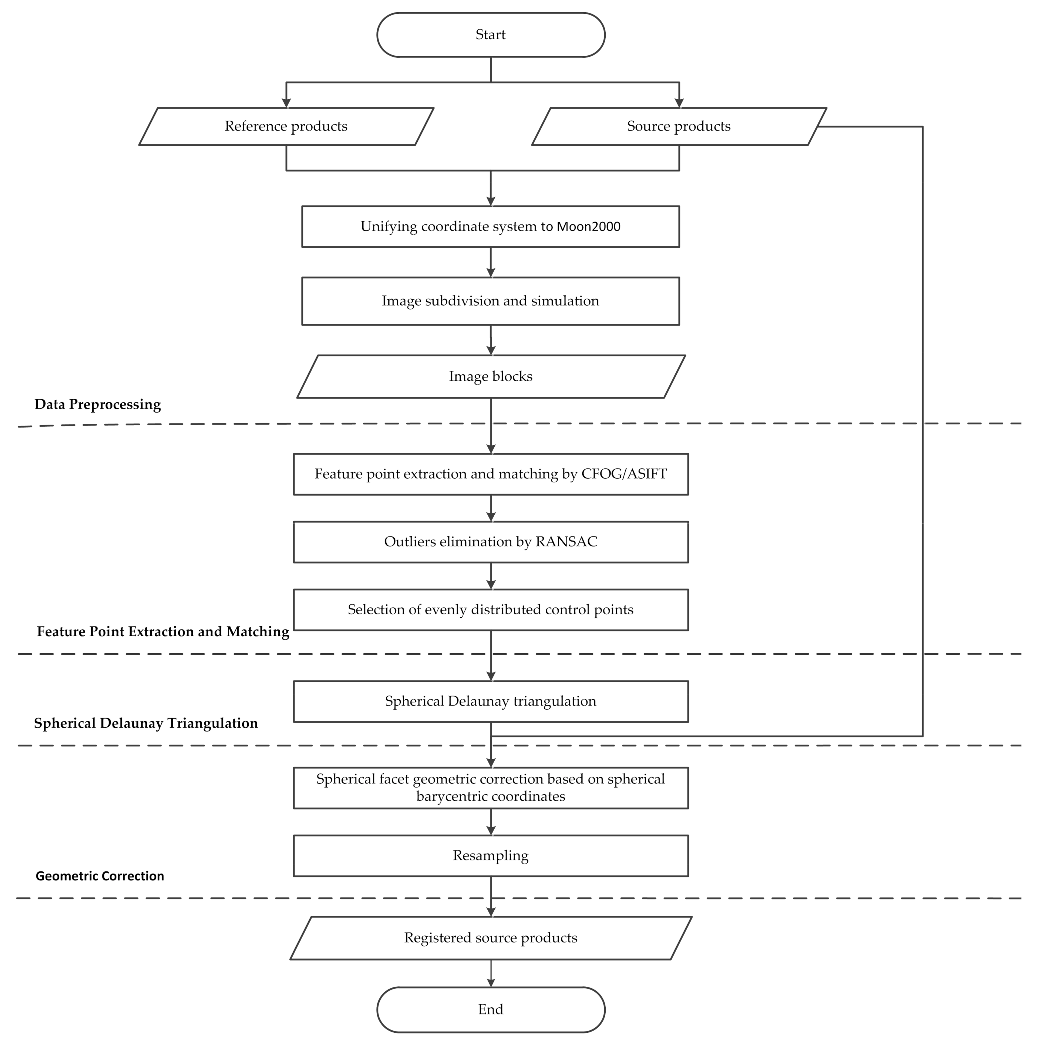
2. Methodology

Figure 1 shows the flowchart of the proposed spherical triangular-mesh-based method, which consists of four major steps; namely, data preprocessing, feature point extraction and matching, spherical Delaunay triangulation, and geometric correction with spherical barycentric coordinates. The technical details are elucidated in the following sub-sections.

2.1. Data Preprocessing

The Moon 2000 planetocentric coordinate system was selected as the spatial reference system in our research as it is most widely used and is convenient for lunar global analysis. If the lunar global mapping products to be processed are not in the Moon 2000 coordinate system, they should first be converted to the Moon 2000 system with longitude and latitude as the unit. After unifying the coordinate system, we subdivide each product into regular blocks in longitude and latitude for efficient handling of large data. In order to avoid resolution loss, there is usually a large amount of redundancy (repeated pixels) in high latitudes in the image files stored in the spherical coordinate system, which will cause difficulties in feature point extraction. Thus, blocks at high latitudes need to be converted to the projected coordinate system (i.e., polar stereographic projection). This map projection process is only used to facilitate feature point extraction and matching. The subsequent Delaunay triangulation and geometric correction are all realized in the spherical coordinate system.

Additionally, when registering two global DEMs or a DEM to lunar imagery, we use the hillshading technique to generate simulated imagery of DEM data [16,20]. The simulated image is a gray-scale representation of the terrain surface under a certain illumination condition (i.e., azimuth and elevation of the Sun), and is similar to a real lunar image. The 3D-3D or 3D-2D matching is then transferred into the 2D-2D matching based on the simulated imagery. We have developed a software tool to create simulated images of DEM data for batch processing based on the hillshading technique and GDAL (Geospatial Data Abstraction Library) open-source library. The solar azimuth angle and solar altitude angle of reference and source DEM data need to be set to be the same, and the default values are 315° and 45°, respectively.

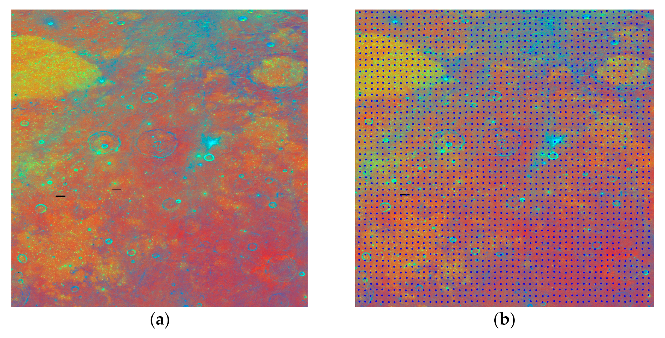
2.2. Feature Point Extraction and Matching

We chose the ASIFT algorithm [24] to extract and match the feature points of DEM simulated images under the same illumination condition. As a variant of SIFT, ASIFT is not only invariant to scale, rotation, and translation, but also invariant to affine transformation. A comparative study has shown that ASIFT outperforms SIFT and SURF in terms of more keypoints and fewer mismatches [61]. A two-resolution scheme further reduces the ASIFT complexity to about twice that of SIFT [24]. In this study, an open-source web code [62] developed by Yu and Morel [63] was used to extract and match the feature points on the simulated images in corresponding blocks.

A fast and robust matching for multimodal remote sensing images proposed by Ye et al. [33] was also adopted in this research, and the software package can be downloaded from the GitHub website [64]. This method first extracts the channel feature of orientated gradient (CFOG) of each pixel to generate the feature representation for each pixel. A similarity measure based on the feature representation is then established in the frequency domain to accelerate the image matching. Subsequently, corresponding feature points between images are detected in a template matching manner.

The random sample consensus (RANSAC) [65] algorithm is used to eliminate mismatches in both of the two methods. Moreover, for lunar global mapping product registration with complex geometric inconsistency, even distribution of control points covering every possible local deformation region is critical. In order to obtain evenly distributed tie points to ensure the uniformity of the spherical triangular mesh, the redundant points are removed from the set of tie points. For this purpose, each block is divided into dense grids, where the point closest to the center of the grid is retained as the control point to construct the spherical triangulation if multiple points exist in a grid.

The settings in the feature point extraction and matching step include search radius (e.g., 100 pixels), template radius (e.g., 100 pixels), grid number (e.g., 225), error elimination threshold (e.g., 2.5 pixels), and so on, which can be set and modified flexibly according to the reference and source data.

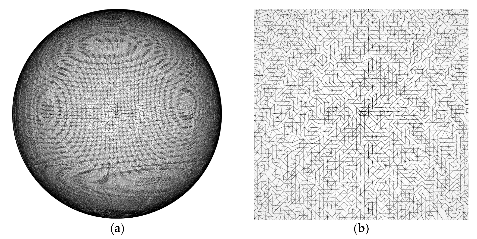
2.3. Spherical Delaunay Triangulation

The construction of a spherical Delaunay triangulation network is an extension of the traditional 2D Delaunay triangulation network. The rules for constructing the 2D Delaunay triangulation are (1) the 2D Delaunay triangulation is unique, and the circumcircle of any triangle does not contain any fourth point; (2) among all possible triangulations, the smallest angle of the Delaunay triangle is the largest.

Specifically, the rules mean that after the diagonals of the convex quadrilateral formed by two adjacent triangles are exchanged with each other, the minimum angle of the six new internal angles no longer increases. By extending the criteria of 2D Delaunay triangulation to the sphere, the following rules [66] can be obtained: (1) the inferior arc surface stretched by the circumscribed circle of any spherical triangle contains no other point; that is, the center of the sphere and all other points are located on the same side of the plane of the triangle; (2) the minimum of the six new interior angles of two adjacent spherical triangles does not increase after their diagonals are swapped.

In this paper, the incremental algorithm is used to generate the spherical Delaunay triangulation. The algorithm was first proposed by Lawson [67] and improved by Bowyer [68]. Renka [69] then proposed a spherical Delaunay triangulation algorithm based on the incremental algorithm. The open-source code for this incremental algorithm is available on the GitHub website [70]. The basic steps of the algorithm are as follows.

(1)

The convex hull H of the spherical scatter point set V is established to enclose all the data points. A convex hull is a minimum convex polyhedron containing a series of known vertices in spatial geometry. In this algorithm, the convex hull consists of eight triangular faces determined by six vertices.

(2)

Find the spherical triangle T that contains the insertion point P in the constructed convex hull H or triangulation network. T is then triangulated by connecting the insertion point P to the three vertices of T to form three new spherical triangles.

(3)

A local optimization process (LOP) is used to optimize the triangle triangulation; that is, by exchanging diagonals to ensure that the triangle formed is a Delaunay triangle.

(4)

Repeat (2) and (3) until the last point has been inserted.

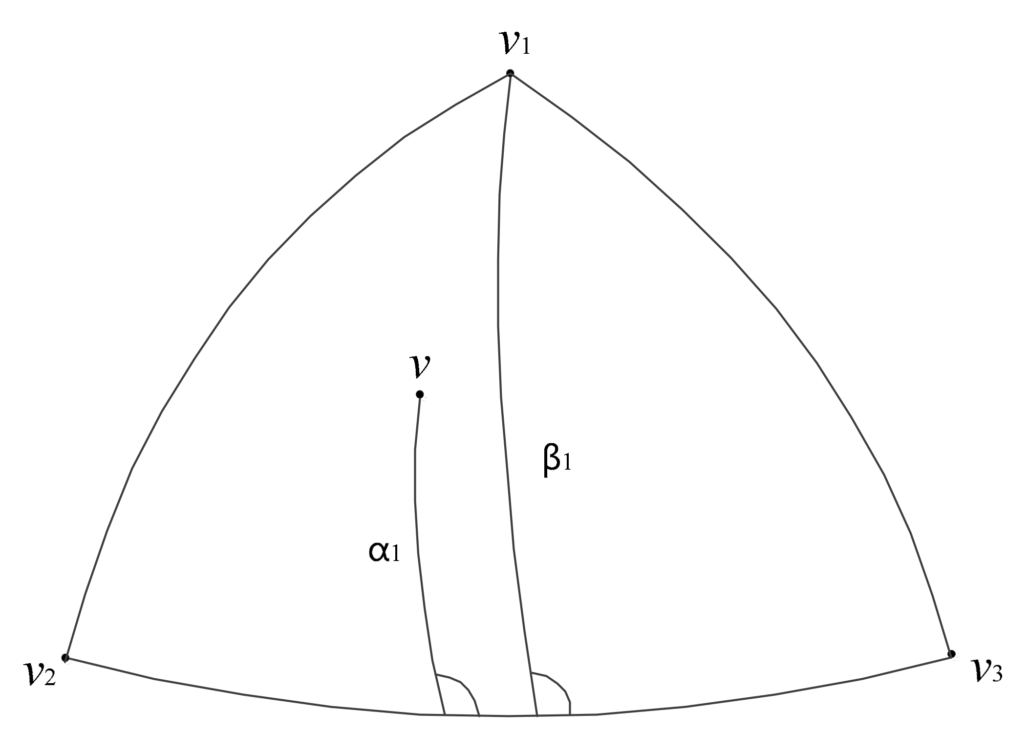
2.4. Spherical Geometric Correction Based on Spherical Barycentric Coordinates

A barycentric coordinate is a special local coordinate, which takes the vertices of a polygon as the reference points to locate an arbitrary point inside the polygon. Barycentric coordinates are widely used in computer graphics and other fields for their excellent characteristics such as normality, linear reconstruction, and affine invariance. In this research, we apply the barycentric coordinates to the deformation of spherical triangular facets.

Barycentric coordinates were first introduced by Möbius [71]. Let T be a triangle with vertices ${\left(v_i\right)}_{i=1,2,3}$. The position of any point $v$ inside the triangle T on the plane ${\mathbb{E}}^2$ can be obtained by taking an adequately weighted sum of the three vertices. These three weight coefficients ${\lambda }_i{\left(v,T\right)}_{i=1,2,3}$ are the barycentric coordinates of the point $v$ in the reference triangle, and the barycentric coordinates are continuous functions that satisfy the following properties.

$$\forall i {\lambda }_i\left(v,T\right) >0;$$

(1)

$${{\displaystyle \sum }}_i{\lambda }_i\left(v,T\right)=1;$$

(2)

$${{\displaystyle \sum }}_i{\lambda }_i\left(v,T\right)v_i=v.$$

(3)

Möbius [72] first extended the concept of barycentric coordinates from a plane to a sphere. Similar to the barycentric coordinates of a planar triangle, the spherical barycentric coordinates represent the position of arbitrary point $v$ on a sphere relative to the three vertices of a reference spherical triangle P. Previous studies [73,74] have shown that, unlike planar triangles, it is impossible for the barycentric coordinates of any point on a spherical triangle to satisfy properties (1), (2), and (3) at the same time. Specifically, properties (2) and (3) are contradictory to each other on spheres. Property (2) satisfies the request that any point $v$ represented by the barycentric coordinates be located in a plane, whereas the property (3) demands that the point $v$ be located on a spherical surface rather than a plane. Consequently, to use the barycentric approach as a solution to the spherical problem, it is essential to relax the above properties to obtain the spherical barycentric coordinates. Alfeld et al. [75] and Langer et al. [74] strictly retained property (3), but relaxed property (2) to

$${{\displaystyle \sum }}_i{\lambda }_i\left(v,P\right) \ge 1;$$

(4)

This is because their main goal was to define curves and surfaces over the sphere. Lei et al. [76] proposed an opposite strategy, which abandons the preservation of property (3) but strictly preserves property (2), dedicated to constructing spherical grid systems. For the problem to be solved in this paper, specifically referring to determining the new position of the sphere point on the transformed sphere surface by the unique spherical barycentric coordinates, it is essential to retain property (3). Hence, we follow the first strategy, retaining property (3) and replacing property (2) with (4).

This paper follows the formula of spherical barycentric coordinates given by Alfeld et al. [75]. Once more, it is assumed that the vertices of a spherical triangle P are the points in the set $V=\left\{v_1,v_2,v_3\right\}$; let $n_i$ denote the unit normal vectors to the planes $P_i=span\left(V\backslash \left\{v_i\right\}\right),i=1,2,3$. For a point $v\in$ sphere $S$, let the angles ${\alpha }_i, {\beta }_i$ be defined by the dot products

$$sin{\alpha }_i≔v·n_i, sin{\beta }_i≔v_i·n_i, i=1,2,3.$$

(5)

where ${\alpha }_i$ represent oriented angles between the vector v and the planes $P_i$, while ${\beta }_i$ are the analogues angles between $v_i$ and $P_i$ (see Figure 2). For nontrivial spherical triangles, $sin{\beta }_i\ne 0,i=1,2,3$. The spherical barycentric coordinates of the point $v\in S$ with respect to the triangle P are given by

$${\lambda }_i\left(v\right)=\frac{sin{\alpha }_i}{sin{\beta }_i}, i=1,2,3.$$

(6)

The main idea of geometric correction based on spherical barycentric coordinates is to establish the transformation relationship between the source spherical triangle and the reference spherical triangle. The vertex of a spherical triangle P is denoted as $V=\left\{v_1,v_2,v_3\right\}$, and the positions of each pixel $v$ inside the spherical triangle are the spherical barycentric coordinates ${\lambda }_i\left(v,P\right)$. P is deformed to form a reference triangle P’ by moving the position of the vertex, the source vertex $V$ corresponds to the new reference vertex $V^{\prime }=\left\{{v_1}^{\prime },{v_2}^{\prime },{v_3}^{\prime }\right\}$, and the internal pixels also change accordingly. The position of each point $v$’ inside the P’ can be calculated using the spherical barycentric coordinates as follows.

$$v^{\prime }={{\displaystyle \sum }}_i{\lambda }_i\left(v,P\right)·v_i^{\prime }, i=1,2,3.$$

(7)

The geometric correction is realized by calculating the transformed position of each pixel of the source data using the above equation for each facet. The final product is generated after resampling.

3. Experimental Results

We performed registration experiments to verify the performance of the proposed high-precision registration method using four different lunar global mapping products; namely, Moon Clementine UVVIS Warped Color Ratio Mosaic 200 m, CE1_TMap_GDOM_120m, SLDEM2015, and CE2TMap2015_DEM_20m. Two separate experiments were conducted to evaluate registration of imagery products and registration of DEMs. In the first experiment, Moon Clementine UVVIS Warped Color Ratio Mosaic 200 m was taken as the reference data and the CE1_TMap_GDOM_120m was taken as source data to be registered to the reference data. The data for the second experiment are both DEM products, with SLDEM2015 and CE2TMap2015_DEM_20m as reference and source data, respectively.

3.1. Experimental Data

The Clementine Ultraviolet-Visible (UVVIS) warped color-ratio mineral map is a false color band ratio image covering the global lunar surface and published by United States Geological Survey (USGS) Astrogeology Science Center. It was generated from the Clementine UVVIS mosaics using three spectral filters (central wavelengths of 415, 750, and 1000 nm) [77,78], and multispectral mosaics with highly accurate radiometric calibrations, photometric corrections, and geodetical controls have been registered to ULCN2005 [4]. The false color band ratio image is a composite image, including the ratio of the 750/415 nm bands used for the red-channel brightness, 750/1000 nm for the green channel, and the 415/750 nm ratio for the blue channel. For detailed information on what color ratios represent, please refer to Lucey et al. [79]. This global product with the spatial resolution of 200 m/pixel is available in GeoTIFF format at the USGS website [80]. Some small gaps in the image are due to lack of coverage in one or more of the bands used in the color ratio.

CE1_TMap_GDOM_120m is a lunar global DOM made of images obtained by a stereo camera with three-line CCDs onboard the CE-1. The intersection angles of the forward and backward relative to the nadir images of the stereo camera are ±16.7°. CE-1 has an orbital altitude of about 200 km and an orbital inclination of nearly 90°. During the flight around the Moon, the three-linear CCD stereo camera takes images in the linear array push-broom way, with a spatial resolution of about 120 m and an image width of about 60 km. The overlap rate of image data in adjacent orbits is more than 40%, and the planimetric positioning accuracy is about 100 m~1.5 km [81]. Li et al. [12] processed the image data according to the mapping specification, carried out photometric correction, improved the consistency of the images, and finally produced a lunar global orthophoto map with a simple cylindrical projection and a spatial resolution of 120 m. The data are provided by the Lunar and Planetary Data Release System [82].

SLDEM2015 is a near-global DEM product constructed by combining the altimeter data from the Lunar Reconnaissance Orbiter Laser Altimeter (LOLA) and the DEM generated by stereo images obtained by SELENE TC. Barker et al. [15] divided the SELENE DEM into 1° × 1° tiles, taking the LOLA point cloud data as reference. Each tile was then adjusted by the tile-averaged transformation parameters (three translation parameters and two tilt parameters) solved by a bounded downhill simplex minimization algorithm. The resultant SLDEM2015 combines the advantages of LOLA’s accurate reference geodetic framework with the high resolution of the SELENE DEM. The SLDEM2015 covers the region between 60°N and 60°S, with a grid spacing of 512 pixels/degree (60 m/pixel at the equator) and a typical vertical accuracy of 3 m–4 m. This DEM product is available for download in GeoTIFF format from the USGS website [83].

CE2TMap2015_DEM_20m is a lunar global DEM, which is a major part of CE2TMap2015 [14]. It was produced from stereo images obtained by the CE-2 stereo camera, using the lunar surface positions of five laser ranging retro reflectors (LRRRs) (Apollo 11, Apollo 14, Apollo 15, Lunokhod 1, and Lunokhod 2) as the absolute control points to realize a seamless mosaic and high-precision absolute positioning [14,84]. CE2TMap2015_DEM_20m has a resolution of 20 m/pixel and 100% coverage of the Moon. It is the highest-resolution lunar global DEM product ever published, and is available through the Lunar and Planetary Data Release System [85]. This DEM product is organized in 188 subdivisions; each subdivision includes a data file (GeoTIFF format), a coordinate information file (tfw), and a projection file (prj) of the same name.

3.2. Data Preprocessing, Matching, and Spherical Delaunay Triangulation Results

In the data preprocessing step, the reference and source products were first divided into regular blocks in longitude and latitude. Within the range of the latitude ±60°, Moon Clementine UVVIS Warped Color Ratio Mosaic 200 m and CE1_TMap_GDOM_120m were divided into 30° × 30° blocks, and SLDEM2015 and CE2TMap2015_DEM_20m were divided into 5° × 5° blocks. For high latitudes and polar regions beyond the ±60° area, the products of the first experiment were converted into Moon stereoscopic north/south pole projection and divided into 18 blocks with the same size.

In experiment 1, the multimodal remote sensing image matching method proposed by Ye et al. [33] was used to match the feature points between corresponding reference and source blocks. The ASIFT algorithm was used to extract and match the feature points of DEM simulated images under the same illumination in experiment 2. The RANSAC algorithm was used to eliminate mismatches in each block. Each block of experiment 1 and experiment 2 was then divided into 50 × 50 and 15 × 15 non-overlapping grids, respectively, and the point closest to the center of each grid was reserved as the control point of the subsequent construction of the triangulated network. Finally, 131,082 and 301,022 control points for experiment 1 and 2 were obtained, respectively. Figure 3 and Figure 4 show the matching results of one typical block in each experiment.

We used the points of the reference image obtained above to construct the spherical Delaunay triangulated network, and the results of experiment 1 are shown in Figure 5. The numbers of spherical triangular facets in experiments 1 and 2 were 262,160 and 602,022, respectively. The spherical Delaunay triangulated network constructed by the source image is the same as that constructed by the reference image, with vertices being replaced by the corresponding vertices in the source image. As a result, based on the corresponding spherical triangular facets, the global registration problem is converted into the local problem. Figure 5 takes experiment 1 as an example to show the results of spherical Delaunay triangulation.

3.3. Registration Results and Analysis

3.3.1. Quantitative Analysis

In this subsection, a quantitative analysis was first conducted to evaluate the registration accuracy. A certain number of randomly distributed points were automatically selected as the checkpoints to assess the geometric displacements before and after the registration, and these checkpoints were selected from the redundant points removed from the tie points set (after outlier elimination) in the matching step of the proposed method. The number of checkpoints was 16,377 and 17,280 for the experiments 1 and 2, respectively. The distribution of the checkpoints is shown in Figure 6.

The geometric displacement, i.e., the planar residual, was evaluated based on the difference in planetocentric coordinates of each checkpoint pair. The planar residual was computed by the following formula:

$${\mathsf{\sigma }}_{\mathrm{p}}=\sqrt{∆{\mathrm{x}}^2+∆{\mathrm{y}}^2,}$$

(8)

$$∆x=\frac{\pi Dcos\left(la{t}_{ref}\right)}{360}∆lon, ∆y=\frac{\pi Dcos\left(la{t}_{ref}\right)}{360}∆lat,$$

$$∆lon=lo{n}_{source}-lo{n}_{ref}, ∆lat=la{t}_{source}-la{t}_{ref}.$$

where $∆lon$ and $∆lat$ are the longitude and latitude residuals of the checkpoints, respectively; $∆x$ and $∆y$, which are converted to meters, are the residuals between the checkpoints; D is the diameter of the Moon; the coordinates of the checkpoints in source data are ($lo{n}_{source}, la{t}_{source}$), and the coordinates of the checkpoints in reference data are ($lo{n}_{ref}, la{t}_{ref}$).

The magnitude and distribution of planar residuals are shown by the color shading maps (Figure 7 and Figure 8) with 1° spacing. Figure 7a shows that the differences between CE1_TMap_GDOM_120m and Clementine UVVIS Warped Color Ratio Mosaic 200 m vary widely, with smaller differences on the lunar near side compared to the far side and smaller residuals in the northern hemisphere compared to the southern. Areas with particularly high differences are clustered in the southern hemisphere (78°E–140°E, 7°N–80°S), and the highest residual is more than 5000 m, which is much larger than the differences of tens of meters in other areas. It is clear from Figure 8a that the differences between CE2TMap2015_DEM_20m and SLDEM2015 near lunar maria are smaller than those of other areas. This is attributed to the fact that five LRRRs with high positioning accuracy were used as control points in CE-2 map production and that the topography of the area is relatively flat. Figure 7b and Figure 8b show that the planar residuals between reference data and source data after registration of both the experiments are greatly reduced, indicating that the proposed method is effective and the registration results are of high precision.

Furthermore, statistics of mean absolute error (MAE) and root-mean-square error (RMSE) of the planar residuals between the checkpoints of reference and source data have been used for quantitative evaluation. The errors are represented both in meters and pixels (with respect to the reference data). The results, given in

Table 1. Quantitative statistics of the planar residuals before and after registration using our proposed method in experiments 1 and 2.

Experiment Group	Registration Status	MAE (m, pixel)	RMSE (m, pixel)
experiment 1	before	2225.0, 11.13	2442.2, 12.21
	after	135.7, 0.68	198.3, 0.99
experiment 2	before	184.5, 3.08	106.5, 1.78
	after	38.5, 0.64	43.0, 0.71

, show that the MEANs and RMSEs are several pixels in experiment 1 and over ten pixels in experiment 2 before registration; the errors are significantly reduced to sub-pixel level after registration in both experiments. The statistical results demonstrate that our proposed method has achieved high precision over the entire lunar globe.

3.3.2. Qualitative Analysis

The performance of the proposed method was also evaluated qualitatively by visual inspection using checkerboard mosaic images, where neighboring squares were taken from the reference product and the source product before and after registration. The details are shown in Figure 9 and Figure 10.

Compared with the checkerboard image before registration (Figure 9c and Figure 10e) showing large deviations at the boundaries of adjacent squares, the regions of the checkerboard image after registration (Figure 9d and Figure 10f) are well overlapped, and the linear features across the boundaries of adjacent squares are continuous. This visually verifies the effectiveness of the proposed registration method.

In principle, the proposed method needs a large number of evenly distributed control points to represent the local variation in geometric inconsistency. Therefore, the quantity and spatial distribution of the extracted control points are crucial to the registration precision of lunar global products with complex local deformation. More control points generally result in higher registration precision, but too many control points will inevitably reduce the efficiency of spherical triangulation and geometric correction. Therefore, the effect of control point density on registration precision needs to be studied in future research.

4. Conclusions

This paper proposed a spherical triangular-mesh-based method for high-precision registration of lunar global mapping products. The proposed method has three main innovations. First, the global spherical registration is not affected by the distortion caused by map projection, especially in high latitude and polar regions. Second, the spherical triangular facets avoid using a single transformation model to register the whole lunar global product, and thus resolve the problem of local geometric distortion. Finally, the local transformation model of spherical barycentric coordinates can achieve high-precision of registration and ensure that the registered product after transformation is continuous at the edges of the spherical triangular mesh.

In the experiments, the performance of the proposed method was evaluated quantitatively and qualitatively. The quantitative results show that the planar residuals between source data and reference data after registration are greatly reduced to sub-pixel level. The qualitative results conducted with the same data are consistent with the quantitative analysis. Both the quantitative and qualitative results show that our proposed method achieved high precision for the registration of lunar global products, confirming the effectiveness of this method. The method can be applied to register global mapping products of the same or different types, e.g., optical image products, spectral image products, and DEM.

References

- Smith, D.E.; Zuber, M.T.; Neumann, G.A.; Lemoine, F.G. Topography of the Moon from the Clementine lidar. J. Geophys. Res. 1997, 102, 1591–1611. [Google Scholar] [CrossRef]
- Robinson, M.S.; McEwen, A.S.; Eliason, E.; Lee, E.M.; Malaret, E.; Lucey, P.G. Clementine UVVIS global mosaic: A new tool for understanding the lunar crust. In Proceedings of the Lunar and Planetary Science Conference, Houston, TX, USA, 15–29 March 1999. [Google Scholar]
- Eliason, E.; Isbell, C.; Lee, E.; Becker, T.; Gaddis, L.; McEwen, A.; Robinson, M. The Clementine UVVIS Global Lunar Mosaic; Lunar and Planetary Institute: Houston, TX, USA, 1999. [Google Scholar]
- Hare, T.M.; Archinal, B.A.; Becker, T.L.; Gaddis, L.R.; Lee, E.M.; Redding, B.L.; Rosiek, M.R. Clementine mosaics warped to ULCN2005 network. In Proceedings of the 39th Annual Lunar and Planetary Science Conference, League City, TX, USA, 10–14 March 2008; p. 2337. [Google Scholar]
- Lee, E.M.; Gaddis, L.R.; Weller, L.; Richie, J.O.; Becker, T.; Shinaman, J.; Rosiek, M.R.; Archinal, B.A. A new Clementine basemap of the Moon. In Proceedings of the 40th Annual Lunar and Planetary Science Conference, The Woodlands, TX, USA, 23–27 March 2009; p. 2445. [Google Scholar]
- WAC Global Morphologic Map. Available online: http://wms.lroc.asu.edu/lroc/view_rdr/WAC_GLOBAL (accessed on 10 April 2018).
- LRO CameraTeam Release High Resolution Global Topographic Map of Moon. Available online: http://www.nasa.gov/mission_pages/LRO/news/lro-topo.html (accessed on 10 April 2018).
- Wagner, R.V.; Speyerer, E.J.; Robinson, M.S.; LROC Team. New mosaicked data products from the LROC team. In Proceedings of the 46th Annual Lunar and Planetary Science Conference, The Woodlands, TX, USA, 16–20 March 2015; p. 1473. [Google Scholar]
- Haruyama, J.; Ohtake, M.; Matsunaga, T.; Otake, H.; Yamamoto, S. Data Products of SELENE (Kaguya) Terrain Camera for Future Lunar Missions. In Proceedings of the 45th Annual Lunar and Planetary Science Conference, The Woodlands, TX, USA, 17–21 March 2014. [Google Scholar]
- Taylor, L.A.; Pieters, C.; Patchen, A.; Taylor, D.S.; Morris, R.V.; Keller, L.P.; McKay, D.S. Mineralogical and chemical characterization of lunar highland soils: Insights into the space weathering of soils on airless bodies. J. Geophys. Res. 2010, 115, E02002. [Google Scholar] [CrossRef]
- Ohtake, M.; Pieters, C.M.; Isaacson, P.; Besse, S.; Green, R.O. One Moon, many measurements 3: Spectral reflectance. Icarus 2013, 226, 364–374. [Google Scholar] [CrossRef]
- Li, C.; Su, Y.; Wen, W.; Bian, W.; Zhao, B.; Yang, J.; Zou, X.; Wang, M.; Xu, C.; Kong, D. The global image of the Moon obtained by the chang’e-1: Data processing and lunar cartography. Sci. China 2010, 53, 1091–1102. [Google Scholar] [CrossRef]
- Li, C.; Ren, X.; Liu, J.; Zou, X.; Mu, L.; Wang, J.; Shu, R.; Zou, Y.; Zhang, H.; Chang, L. Laser altimetry data of chang’e-1 and the global lunar dem model. Sci. China Ser. D Earth Sci. 2010, 40, 281–293. [Google Scholar] [CrossRef]
- Li, C.; Liu, J.; Ren, X.; Yan, W.; Zuo, W.; Mou, L.; Zhang, H.; Su, Y.; Wen, W.; Tan, X.; et al. Lunar Global High-precision Terrain Reconstruction Based on Chang’e-2 Stereo Images. Geomat. Inf. Sci. Wuhan Univ. 2018, 43, 485–495. [Google Scholar]
- Barker, M.K.; Mazarico, E.; Neumann, G.A.; Zuber, M.T.; Haruyama, J.; Smith, D.E. A new lunar digital elevation model from the Lunar Orbiter Laser Altimeter and SELENE Terrain Camera. Icarus 2016, 273, 346–355. [Google Scholar] [CrossRef] [Green Version]
- Xin, X.; Liu, B.; Di, K.; Yue, Z.; Gou, S. Geometric quality assessment of chang’e-2 global DEM product. Remote Sens. 2020, 12, 526. [Google Scholar] [CrossRef] [Green Version]
- Di, K.; Liu, B.; Xin, X.; Yue, Z.; Ye, L. Advances and applications of lunar photogrammetric mapping using orbital images. Acta Geod. Et Cartogr. Sin. 2019, 48, 1562. [Google Scholar]
- Kirk, R.L.; Archinal, B.A.; Gaddis, L.R.; Rosiek, M.R. Lunar Cartography: Progress in the 2000s and prospects for the2010s. In Proceedings of the 2012 ISPRS-International Archives of the Photogrammetry Remote Sensing and Spatial Information Sciences, Melbourne, Australia, 25 August–1 September 2012; Volume XXXIX-B4, pp. 489–494. [Google Scholar]
- Wu, B.; Guo, J.; Hu, H.; Li, Z.; Chen, Y. Co-registration of lunar topographic models derived from Chang’E-1, SELENE, and LRO laser altimeter data based on a Novel surface matching method. Earth Planet Sci. Lett. 2013, 364, 68–84. [Google Scholar] [CrossRef]
- Xin, X.; Liu, B.; Di, K.; Jia, M.; Oberst, J. High-precision co-registration of orbiter imagery and digital elevation model constrained by both geometric and photometric information. ISPRS J. Photogramm. Remote Sens. 2018, 144, 28–37. [Google Scholar] [CrossRef]
- Zitova, B.; Flusser, J. Image registration methods: A survey. Image Vis. Comput. 2003, 21, 977–1000. [Google Scholar] [CrossRef] [Green Version]
- Li, B.; Wei, W.; Hao, Y. Automatic registration of multisensor images with affine deformation based on triangle area representation. J. Electron. Imaging 2013, 22, 3002. [Google Scholar] [CrossRef]
- Lowe, D.G. Distinctive image features from scale-invariant keypoints. Int. J. Comput. Vis. 2004, 60, 91–110. [Google Scholar] [CrossRef]
- Morel, J.M.; Yu, G. ASIFT: A New Framework for Fully Affine Invariant Image Comparison. SIAM J. Imaging Sci. 2009, 2, 438–469. [Google Scholar] [CrossRef]
- Bay, H.; Tuytelaars, T.; Van Gool, L. Surf: Speeded up robust features. In Proceedings of the European Conference on Computer Vision, Graz, Austria, 7–13 May 2006; pp. 404–417. [Google Scholar]
- Yi, Z.; Zhiguo, C.; Yang, X. Multi-spectral remote image registration based on SIFT. Electron. Lett. 2008, 44, 107–108. [Google Scholar] [CrossRef]
- Sedaghat, A.; Mokhtarzade, M.; Ebadi, H. Uniform robust scale-invariant feature matching for optical remote sensing images. IEEE Trans. Geosci. Remote Sens. 2011, 49, 4516–4527. [Google Scholar] [CrossRef]
- Fan, J.; Yan, W.; Ming, L.; Liang, W.; Cao, Y. Sar and optical image registration using nonlinear diffusion and phase congruency structural descriptor. IEEE Trans. Geosci. Remote Sens. 2018, 56, 5368–5379. [Google Scholar] [CrossRef]
- Sun, H.; Lei, L.; Zou, H.; Wang, C. Multimodal remote sensing image registration using multiscale self-similarities. In Proceedings of the IEEE International Conference on Computer Vision in Remote Sensing, Xiamen, China, 16–18 December 2012; pp. 199–202. [Google Scholar]
- Sedaghat, A.; Ebadi, H. Distinctive order based self-similarity descriptor for multi-sensor remote sensing image matching. ISPRS J. Photogramm. Remote Sens. 2015, 108, 62–71. [Google Scholar] [CrossRef]
- Xiong, X.; Xu, Q.; Jin, G.; Zhang, H.; Gao, X. Rank-based local self-similarity descriptor for optical-to-sar image matching. IEEE Geosci. Remote Sens. Lett. 2019, 17, 1742–1746. [Google Scholar] [CrossRef]
- Ye, Y.; Shan, J.; Bruzzone, L.; Shen, L. Robust registration of multimodal remote sensing images based on structural similarity. IEEE Trans. Geosci. Remote Sens. 2017, 55, 2941–2958. [Google Scholar] [CrossRef]
- Ye, Y.; Bruzzone, L.; Shan, J.; Bovolo, F.; Zhu, Q. Fast and Robust Matching for Multimodal Remote Sensing Image Registration. IEEE Trans. Geosci. Remote Sens. 2019, 57, 9059–9070. [Google Scholar] [CrossRef] [Green Version]
- Wang, G.; Chen, Y. Robust feature matching using guided local outlier factor. Pattern Recognit. 2021, 117, 107986. [Google Scholar] [CrossRef]
- Liu, Y.; Li, Y.; Dai, L.; Yang, C.; Wei, L.; Lai, T.; Chen, R. Robust feature matching via advanced neighborhood topology consensus. Neurocomputing 2021, 421, 273–284. [Google Scholar] [CrossRef]
- Li, G.; Yu, L.; Fei, S. A deep-learning real-time visual slam system based on multi-task feature extraction network and self-supervised feature points. Measurement 2021, 168, 108403. [Google Scholar] [CrossRef]
- Song, Z.; Zhou, S.; Guan, J. A novel image registration algorithm for remote sensing under affine transformation. IEEE Trans. Geosci. Remote Sens. 2014, 52, 4895–4912. [Google Scholar] [CrossRef]
- Dai, X.; Khorram, S. A feature-based image registration algorithm using improved chain-code representation combined with invariant moments. IEEE Trans. Geosci. Remote Sens. 1999, 37, 2351–2362. [Google Scholar]
- Moigne, J.L. Introduction to remote sensing image registration. In Proceedings of the International Geoscience and Remote Sensing Symposium. Software Engineering Division, NASA Goddard Space Flight Center, Greenbelt, MD, USA, 23–28 July 2017; pp. 2565–2568. [Google Scholar]
- Wong, A.; Clausi, D.A. Arrsi: Automatic registration of remote-sensing images. IEEE Trans. Geosci. Remote Sens. 2007, 45, 1483–1493. [Google Scholar] [CrossRef]
- Gong, M.; Zhao, S.; Jiao, L.; Tian, D.; Wang, S. A novel coarse-to-fine scheme for automatic image registration based on SIFT and mutual information. IEEE Trans. Geosci. Remote Sens. 2014, 52, 4328–4338. [Google Scholar] [CrossRef]
- Liang, J.; Liu, X.; Huang, K.; Li, X.; Wang, D.; Wang, X. Automatic registration of multisensor images using an integrated Spatial and Mutual Information (SMI) metric. IEEE Trans. Geosci. Remote Sens. 2014, 52, 603–615. [Google Scholar] [CrossRef]
- Goshtasby, A. Piecewise linear mapping functions for image registration. Pattern Recognit. 1986, 19, 459–466. [Google Scholar] [CrossRef]
- Goshtasby, A. Piecewise cubic mapping functions for image registration. Pattern Recognit. 1987, 20, 525–533. [Google Scholar] [CrossRef]
- Goshtasby, A. Image registration by local approximation methods. Image Vis. Comput. 1988, 6, 255–261. [Google Scholar] [CrossRef]
- Flusser, J. An adaptive method for image registration. Pattern Recognit. 1992, 25, 45–54. [Google Scholar] [CrossRef]
- Goshtasby, A. Registration of images with geometric distortions. IEEE Trans. Geosci. Remote Sens. 1988, 26, 60–64. [Google Scholar] [CrossRef]
- Bookstein, F.L. Principal warps: Thin-plate splines and the decomposition of deformations. IEEE Trans. Pattern Anal. Mach. Intell. 1989, 11, 567–585. [Google Scholar] [CrossRef] [Green Version]
- Bentoutou, Y.; Taleb, N.; Kpalma, K.; Ronsin, J. An automatic image registration for applications in remote sensing. IEEE Trans. Geosci. Remote Sens. 2005, 43, 2127–2137. [Google Scholar] [CrossRef]
- Di, K.; Jia, M.; Xin, X.; Wang, J.; Liu, B.; Li, J.; Xie, J.; Liu, Z.; Peng, M.; Yue, Z.; et al. High-resolution large-area digital orthophoto map generation using lroc nac images. Photogramm. Eng. Remote Sens. 2019, 85, 481–491. [Google Scholar] [CrossRef]
- Ehlers, M.; Fogel, D.N. High-precision geometric correction of airborne remote sensing revisited: The multiquadric interpolation. Proc. SPIE Int. Soc. Opt. Eng. 1994, 2315, 814–824. [Google Scholar]
- Zagorchev, L.; Goshtasby, A. A comparative study of transformation functions for nonrigid image registration. IEEE Trans. Image Process. 2006, 15, 529–538. [Google Scholar] [CrossRef]
- Zhang, Z.; Zhang, J. Facet based differential registration of remote sensing images. In Proceedings of the International Geoscience and Remote Sensing Symposium, Sydney, NSW, Australia, 9–13 July 2001; pp. 712–714. [Google Scholar]
- Yu, L.; Zhang, D.; Holden, E. A fast and fully automatic registration approach based on point features for multi-source remote-sensing images. Comput. Geosci. 2008, 34, 838–848. [Google Scholar] [CrossRef]
- Arevalo, V.; Gonzalez, J. Improving piecewise linear registration of high-resolution satellite images through mesh optimization. IEEE Trans. Geosci. Remote Sens. 2008, 46, 3792–3803. [Google Scholar] [CrossRef]
- Lin, X.; Zhang, Y.; Yang, Y. Application of Triangulation-Based Image Registration Method in the Remote Sensing Image Fusion. In Proceedings of the International Conference on Environmental Science and Information Application Technology, Wuhan, China, 4–5 July 2009; pp. 501–504. [Google Scholar]
- Xie, J.; Li, B.; Han, W.; Bao, J.; Gu, F.; Guo, F. A tiny facet primitive remote sensing image registration method based on SIFT key points. In Proceedings of the 2012 International Symposium on Instrumentation & Measurement, Sensor Network and Automation (IMSNA), Sanya, China, 25–28 August 2012; pp. 138–141. [Google Scholar]
- Han, Y.; Byun, Y.; Choi, J.; Han, D.; Kim, Y. Automatic registration of high-resolution images using local properties of features. Photogramm. Eng. Remote Sens. 2012, 78, 211–221. [Google Scholar] [CrossRef]
- Han, Y.; Choi, J.; Byun, Y.; Kim, Y. Parameter optimization for the extraction of matching points between high-resolution multisensor images in urban areas. IEEE Trans. Geosci. Remote Sens. 2014, 52, 5612–5621. [Google Scholar] [CrossRef]
- Lee, D.T.; Schachter, B.J. Two algorithms for constructing a Delaunay triangulation. Internat. J. Comput. Inform. Sci. 1980, 9, 219–242. [Google Scholar] [CrossRef]
- Wu, J.; Cui, Z.; Sheng, V.S.; Zhao, P.; Su, D.; Gong, S. A comparative study of sift and its variants. Meas. Sci. Rev. 2013, 13, 123–131. [Google Scholar] [CrossRef] [Green Version]
- ASIFT: An Algorithm for Fully Affine Invariant Comparison. Available online: http://demo.ipol.im/demo/my_affine_sift/ (accessed on 13 March 2022).
- Yu, G.; Morel, J.M. ASIFT: An Algorithm for Fully Affine Invariant Comparison. Image Process. Line 2011, 1, 11–38. [Google Scholar] [CrossRef] [Green Version]
- CFOG. Available online: https://github.com/yeyuanxin110/CFOG (accessed on 13 March 2022).
- Fischler, M.A.; Bolles, R.C. Random Sample Consensus: A Paradigm for Model Fitting with Applications to Image Analysis and Automated Cartography. Read. Comput. Vis. 1987, 24, 726–740. [Google Scholar] [CrossRef]
- Zhou, L.; Huang, D.; Li, C.; Zhou, D. Algorithm for gps network construction based on spherical delaunay triangulated irregular network. Xinan Jiaotong Daxue Xuebao J. Southwest Jiaotong Univ. 2007, 42, 380–383. [Google Scholar]
- Lawson, C.L. Software for C1 Surface Interpolation. In Proceedings of the Symposium Conducted by the Mathematics Research Center, the University of Wisconsin–Madison, Madison, WI, USA, 28–30 March 1977; pp. 161–194. [Google Scholar]
- Bowyer, A. Computing Dirichlet tessellations. Comput. J. 1981, 24, 162–166. [Google Scholar] [CrossRef] [Green Version]
- Robert, J.R. Algorithm 772: STRIPACK: Delaunay triangulation and Voronoi diagram on the surface of a sphere. ACM Trans. Math. Softw. 1997, 23, 416–434. [Google Scholar]
- DelaunayTriangulation. Available online: https://github.com/xialinbo/DelaunayTriangulation (accessed on 13 March 2022).
- Möbius, A.F. Der Barycentrische Calcul; Johann Ambrosius Barth: Leipzig, Germany, 1827. [Google Scholar]
- Möbius, A.F. Über Eine Neue Behandlungsweise der Analytischen Sphärik; Weidmann: Leipzig, Germany, 1846. [Google Scholar]
- Bronw, J.; Worsey, A. Problems with defining barycentric coordinates for the sphere. RAIRO Modélisation Mathématique Et Anal. Numérique 1992, 26, 37–49. [Google Scholar]
- Langer, T.; Belyaev, A.; Seidel, H.P. Spherical barycentric coordinates. In Proceedings of the 4th Eurographics Symposium on Geometry Processing (SGP ’06), Cagliari, Italy, 26–28 June 2006; pp. 81–88. [Google Scholar]
- Alfeld, P.; Neamtu, M.; Schumaker, L.L. Bernstein-Bézier polynomials on spheres and sphere-like surfaces. Comput. Aided Geom. Des. 1996, 13, 333–349. [Google Scholar] [CrossRef]
- Lei, K.; Qi, D.; Tian, X. A new coordinate system for constructing spherical grid systems. Appl. Sci. 2020, 10, 655. [Google Scholar] [CrossRef] [Green Version]
- Nozette, S.; Rustan, P.; Pleasance, L.P.; Kordas, J.F.; Lewis, I.T.; Park, H.S.; Priest, R.E. The Clementine Mission to the Moon: Scientific Overview. Science 1994, 266, 1835–1839. [Google Scholar] [CrossRef] [PubMed] [Green Version]
- McEwen, A.S.; Robinson, M.S. Mapping of the Moon by Clementine. Adv. Space Res. 1997, 19, 1523–1533. [Google Scholar] [CrossRef]
- Lucey, P.G.; Blewett, D.T.; Taylor, G.J.; Hawke, B.R. Imaging of lunar surface maturity. J. Geophys. Res. 2000, 105, 20377–20386. [Google Scholar] [CrossRef]
- Moon Clementine UVVIS Warped Color Ratio Mosaic 200m v1. Available online: https://astrogeology.usgs.gov/search/map/Moon/Clementine/UVVIS/Lunar_Clementine_UVVIS_Warp_ClrRatio_Global_200m (accessed on 13 March 2022).
- Zhao, B.; Yang, J.; Wen, D.; Gao, W.; Ruan, P.; He, Y. Design and On-orbit Measurement of Chang’ E-1 Satellite CCD Stereo Camera. Spacecr. Eng. 2009, 18, 30–36. [Google Scholar]
- CE1_TMap_GDOM_120m. Available online: https://clpds.bao.ac.cn/ce5web/searchOrder_hyperSearchData.search?pid=CE1/CCD/level/DOM-120m (accessed on 13 March 2022).
- SLDEM2015. Available online: https://astrogeology.usgs.gov/search/map/Moon/LRO/LOLA/Lunar_LRO_LrocKaguya_DEMmerge_60N60S_512ppd (accessed on 13 March 2022).
- Ren, X.; Liu, J.; Li, C.; Li, H.; Yan, W.; Wang, F.; Wang, W.; Zhang, X.; Gao, X.; Chen, W. A global adjustment method for photogrammetric processing of Chang’E-2 stereo images. IEEE Trans. Geosci. Remote Sens. 2019, 57, 6832–6843. [Google Scholar] [CrossRef]
- CE2TMap2015_DEM_20m. Available online: https://clpds.bao.ac.cn/ce5web/searchOrder_hyperSearchData.search?pid=CE2/CCD/level/DEM-20m (accessed on 13 March 2022).