Article

Modeling Forest Canopy Cover: A Synergistic Use of Sentinel-2, Aerial Photogrammetry Data, and Machine Learning

by
Vahid Nasiri
1,
Ali Asghar Darvishsefat
1,
Hossein Arefi
2,
Verena C. Griess
3,
Seyed Mohammad Moein Sadeghi
4 and
Stelian Alexandru Borz
4,*
1
Department of Forestry and Forest Economics, Faculty of Natural Resources, University of Tehran, Karaj 1417643184, Iran
2
Department of Technology, Mainz University of Applied Sciences, 55128 Mainz, Germany
3
Department of Environmental System Sciences, Institute of Terrestrial Ecosystems, ETH Zürich, 8092 Zurich, Switzerland
4
Department of Forest Engineering, Forest Management Planning and Terrestrial Measurements, Faculty of Silviculture and Forest Engineering, Transilvania University of Brasov, 500123 Brasov, Romania
*
Author to whom correspondence should be addressed.
Submission received: 2 February 2022 / Revised: 1 March 2022 / Accepted: 15 March 2022 / Published: 17 March 2022
(This article belongs to the Special Issue UAV Applications for Forest Management: Wood Volume, Biomass, Mapping)

Abstract

:
Forest canopy cover (FCC) is an important ecological parameter of forest ecosystems, and is correlated with forest characteristics, including plant growth, regeneration, biodiversity, light regimes, and hydrological properties. Here, we present an approach of combining Sentinel-2 data, high-resolution aerial images, and machine learning (ML) algorithms to model FCC in the Hyrcanian mixed temperate forest, Northern Iran. Sentinel-2 multispectral bands and vegetation indices were used as variables for modeling and mapping FCC based on UAV ground truth to a wider spatial extent. Random forest (RF), support-vector machine (SVM), elastic net (ENET), and extreme gradient boosting (XGBoost) were the ML algorithms used to learn and generalize on the remotely sensed variables. Evaluation of variable importance indicated that vegetation indices including NDVI, NDVI-A, NDRE, and NDI45 were the dominant predictors in most of the models. Model accuracy estimation results showed that among the tested models, RF (R2 = 0.67, RMSE = 18.87%, MAE = 15.35%) and ENET (R2 = 0.63, RMSE = 20.04%, MAE = 16.44%) showed the best and the worst performance, respectively. In conclusion, it was possible to prove the suitability of integrating UAV-obtained RGB images, Sentinel-2 data, and ML models for the estimation of FCC, intended for precise and fast mapping at landscape-level scale.

1. Introduction

Forest canopy cover (FCC) is an essential forest inventory parameter that has always been used to assess forest disturbances such as forest fragmentation and degradation [1,2]. There is evidence that FCC has a strong relationship with ecohydrological processes [3,4], and plays an important role in forest inventory programs [5,6]. For example, in water management studies, FCC has been widely used to model water cycling and sedimentation [7,8]. In other applications, FCC has been used in forest health assessment [9,10], as well as seedling growth and survival studies [11,12]. Moreover, FCC was found to be an indicator of species richness in forest ecosystems [13,14], wildlife habitats [15,16], and wildfire risk [17,18]. Traditional approaches to FCC modeling include the use of predictive models, where canopy cover is derived from stand attributes such as the diameter at breast height (DBH) and basal area, which are measured or estimated by ground-based inventories [5,19,20], or the use of methods such as those based on hemispherical canopy photography [3,21] and densitometers [22]. In the past decade, remote sensing methods have become the most widely used approach to FCC modeling, e.g., [9,23,24,25,26]. In this regard, different types of remotely sensed datasets—such as optical satellite images and space-borne radar [27,28], LiDAR point clouds [29,30,31], and aerial imagery—have been used [29,32]. For example, Lima et al. [30] used Landsat satellite images and confirmed their excellent performance in long-term FCC monitoring. Karlson et al. [33] used spectral and textural features from the WorldView-2 and Landsat-8 images; according to their findings, the most significant features in FCC mapping were the gray-level co-occurrence matrix (GLCM) and normalized difference vegetation index (NDVI). Jin et al. [34] proposed a hybrid model that combines a 3D radiative transfer model and a transfer-learning-based convolutional neural network (T-CNN) to estimate FCC from China’s GaoFen-2 satellite (1 m resolution with 4 bands) in North China, and reported a high coefficient of determination (R2 = 0.83). Ganz et al. [35] produced FCC maps using aerial and Sentinel-2 satellite images, and reported a high percentage of agreement (95.2%). Hua and Zhao [36] used red-edge bands based on Sentinel-2 satellite images to estimate FCC; the results showed that the red-edge bands could successfully improve the accuracy of FCC estimation models for varying FCC classes. Imagery from Sentinel-2 sensors further improved the information available for FCC assessment. Sentinel-2 imagery is freely available, and provides spectral information in the visible, red-edge, near-infrared (NIR), and shortwave infrared (SWIR) spectra [24,30,35,36,37,38,39]. An accurate and suitable canopy cover classification requires sufficient training and validation samples [40]. In previous studies, these samples were collected in the field either directly or indirectly, but field measurements have been constrained by the technological and logistical limitations and costs, respectively [41,42]. The development of modern commercial sensors—such as lightweight multispectral, hyperspectral, and LiDAR sensors, positioning systems, and unmanned aerial vehicle (UAV) platforms—provides new opportunities to overcome these limitations [43,44,45].
Keeping in mind the goal of an accurate assessment that does not require a ground truth, this research aimed at answering the following questions: (1) which machine learning (hereafter referred to as ML) model might be the most suitable tool for predicting FCC? (2) What relationship exists between Sentinel-2 vegetation indices and UAV-based FCC? (3) Can Sentinel-2 spectral features and vegetation indices, in combination with UAV-based reference data and ML models, provide a suitable tool for FCC mapping at the landscape level? To answer these research questions, we first propose a new method for FCC modeling based on RGB images obtained from UAV and Sentinel-2 satellite data. Then, we evaluate the potential of Sentinel-2 satellite images in FCC modeling and, finally, we compare the performance of four supervised ML algorithms for FCC prediction.

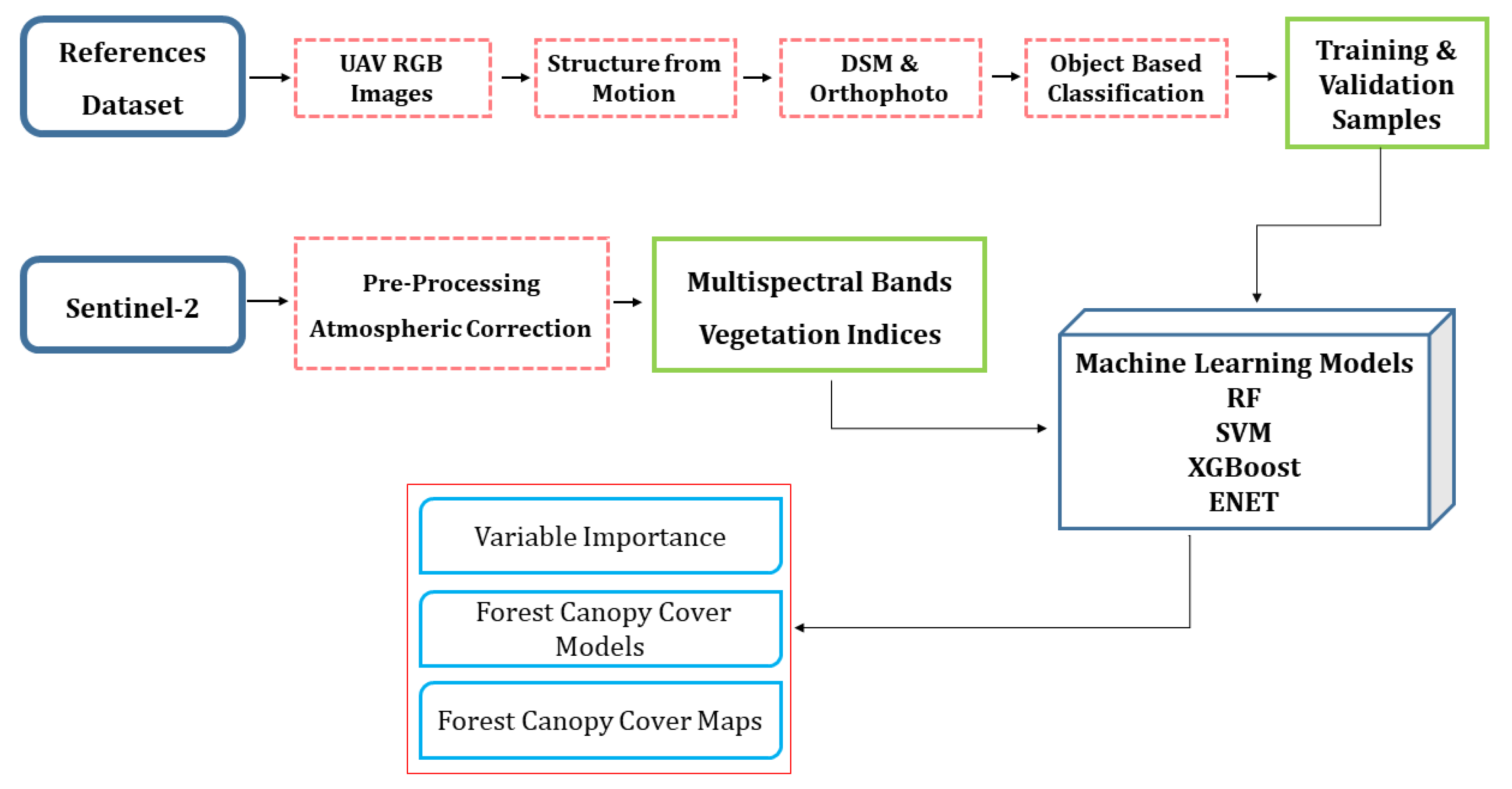
2. Materials and Methods
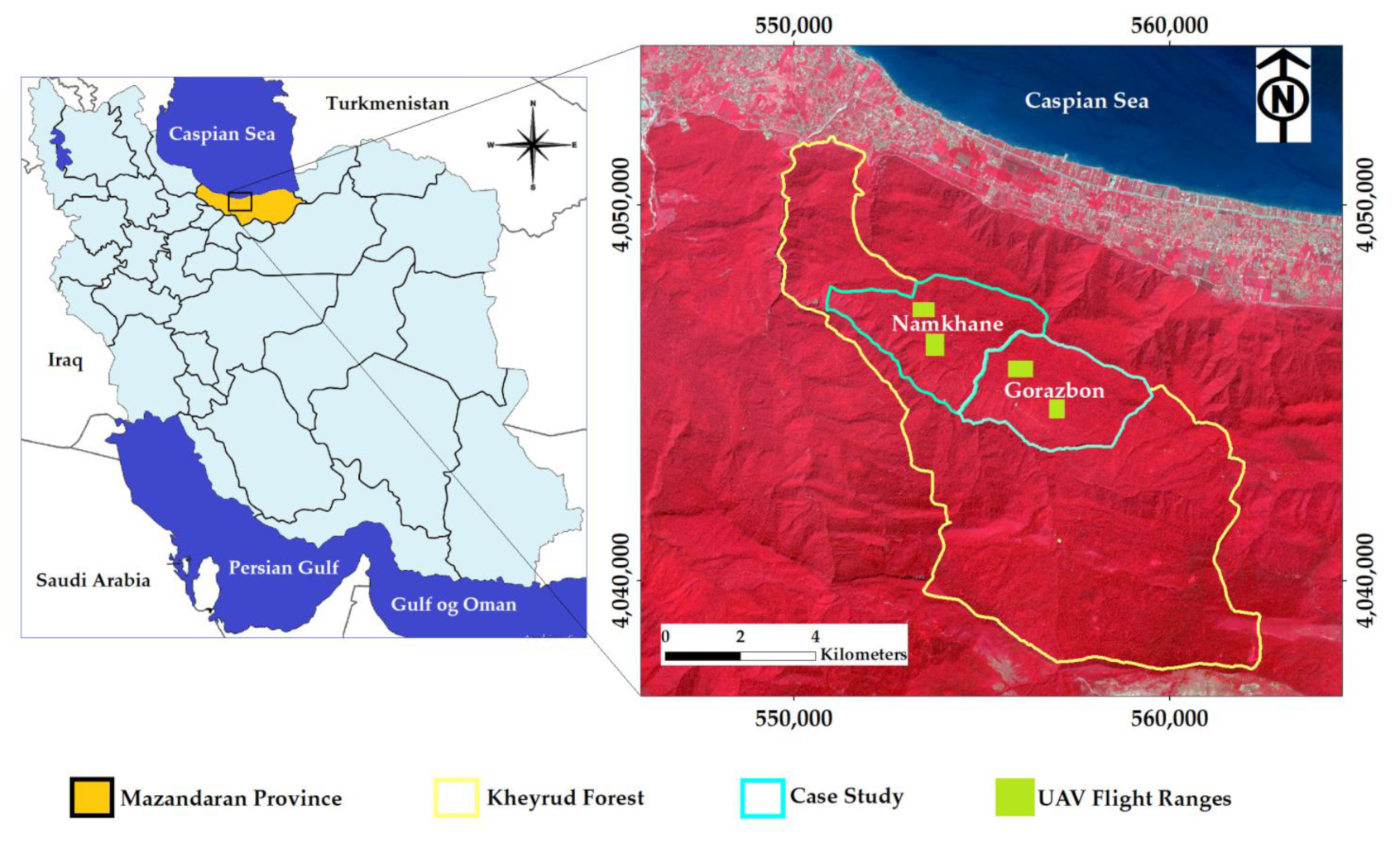
2.1. Study Area

The study area is located within the Kheyrud Experimental Forest, with a total area of approximately 20 km2. The area spreads across both Namkhane (Latitude 36°54′43″ to 36°57′72″N; Longitude 51°56′85″ to 51°63′40″E; WGS84—Universal Mercator projection; elevation in the district ranges from 0 to 1350 m above sea level) and Gorazbon (Latitude 36°53′48″ to 36°56’36”N; Longitude 51°60’72” to 51°66’51”E; WGS84; elevation in the district ranges from 554 to 1489 m above sea level) districts within Mazandaran Province, Northern Iran (Figure 1), also known as the Hyrcanian region. Hyrcanian mixed temperate forests form a unique forested massif that stretches for 850 km along the southern coast of the Caspian Sea and covers over 19,000 km2 [1,46]. These forests were designated as a UNESCO World Heritage Site in 2019 [47]. Annual precipitation fluctuates between 1300 and 1600 mm, with minimal rainfall occurring mid-summer [46]. In the study region, dominant tree species include common hornbeam (Carpinus betulus), oriental beech (Fagus orientalis), chestnut-leaved oak (Quercus castaneifolia), Caucasian alder (Alnus subcordata), velvet maple (Acer velutinum), and Persian ironwood (Parrotia persica) [48].

2.2. RGB Imagery Obtained via UAV Multispectral Camera

An octocopter developed by the University of Tehran was used to fly over the study area in August 2018. We carried out the flights in August, bearing in mind the stability in FCC development as specific to this period. Four flights (Table 1) were conducted in order to collect samples in such a way that the flight ranges and the resulting samples reflected the diversity of FCC in our case study. The UAV was equipped with a global navigation satellite system (GNSS) and an inertial measurement unit (IMU) in order to enable georeferencing of all images obtained. RGB color imagery (red–green–blue) in the range of 350 to 650 nm was obtained using a MAPIR Survey1 Visible Light Camera (San Diego, CA, USA). This camera has a resolution of 4032 by 3024 pixels, and captures images at f/2.8, with a field of view (FOV) of 60° and a focal length of 4 mm. The camera shutter was set in the automatic mode, with an interval of one image per second. All images were captured with 80% overlap (side and forward). The theoretical ground surface distance (GSD) was estimated at 5 cm. Four ground control points (GCPs) were placed at the corners of each flight range to help increase the accuracy in the data processing phase; their locations were determined using a Trimble R3 differential GPS (DGNSS) (Trimble Navigation Limited, CA, USA). Error information associated with GCPs during georeferencing is shown in Table 1.
Orthophotos with a resolution of 5 cm were generated following the structure from motion (SfM) photogrammetric range imaging technique, based on standardized steps that included image alignment, building of dense point clouds, digital surface model (DSM) construction, and orthophoto generation by means of Agisoft Photoscan Professional software (Ver. 1.2.6) [49]. Table 2 summarizes the most important parameters of the photogrammetric data-processing workflow. The main characteristics and technical specifications of the UAV are given in Table 3.

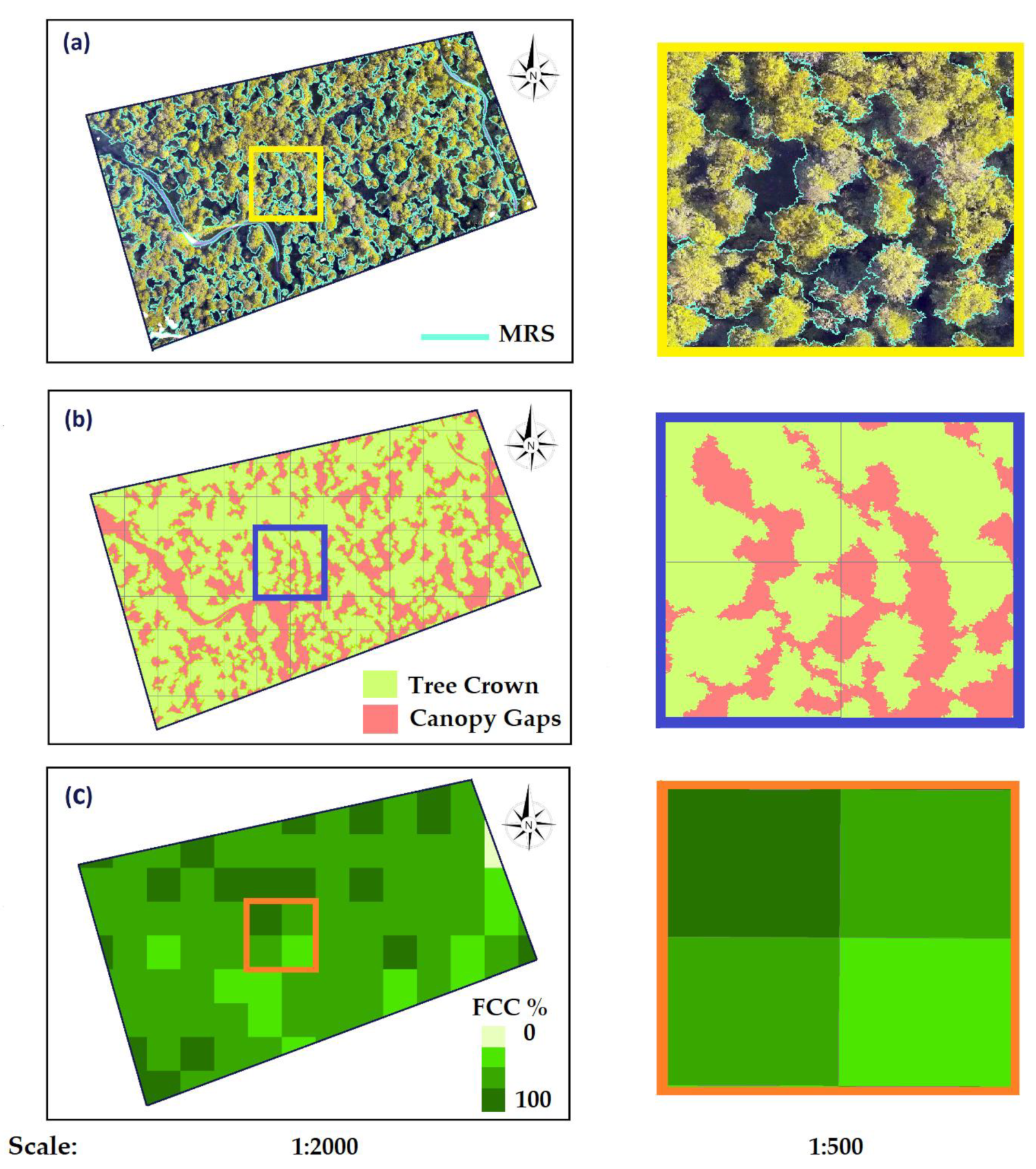
2.3. Reference Dataset

The reference FCC maps were developed based on high-resolution UAV orthophotos and DSMs extracted from UAV images. To enable an object-based image analysis (OBIA), the tree crown borders were delineated using the eCognition Developer software (Ver. 8.7) [50]. To segment the image into homogeneous objects and determine tree crown borders, image segmentation following the multiresolution segmentation (MRS) method was carried out using the UAV-obtained multispectral RGB orthophotos and the DSM (Figure 2a). The MRS parameters were optimized by applying a trial-and-error approach. Segmented images were then classified as either tree crowns or canopy gaps using the nearest neighbor classification (NNC) technique (Figure 2b). The canopy gap class included understory vegetation, bare land, and forest roads. A grid with 50 × 50 m cell size was placed over the maps to determine FCC, and cells belonging to each class were counted. FCC diversity and individual tree crown attributes (such as crown perimeter) are the most important factors that can effectively determine the grid’s cell size. In uneven, mature, dense, and heterogeneous forests (such as our study area), most individuals have large and wide crowns and small gaps between the canopies. Therefore, it is impossible to use a small grid cell size to measure the FCC percentage reliably. We selected the grid cell size by testing different values (10 to 50 m). Finally, the FCC was calculated based on Equation (1)
FCC ( % ) = Area   of   tree   crowns Area   of   each   cell × 100
The resulting map based on this process is shown in Figure 2c for one of our flight missions. A total of 240 FCC samples was generated based on UAV aerial images and the abovementioned workflow.

2.4. Processing of Sentinel-2 Imagery and Feature Extraction

Sentinel-2 level-1C cloud-free top-of-atmosphere (TOA) images were used, which were temporarily as consistent as possible with the performed UAV surveys. The atmospheric correction processor Sen2Cor was used to correct images from the effects of the atmosphere and derive level-2A bottom-of-atmosphere (BOA) images [51,52]. Due to the differences in pixel resolution, all Sentinel-2 bands were resampled to a 10 m resolution. Considering the heterogeneity of both canopy structures and tree species in the study area, suitable vegetation indices were required. The high spectral resolution of Sentinel-2 imagery allowed us to generate a diversity of vegetation indices. In this regard, different vegetation indices based on visible, NIR, and red-edge bands were calculated (Table 4). The process was carried out using the Sentinel Application Platform (SNAP)—open-source software provided by the European Space Agency [53].

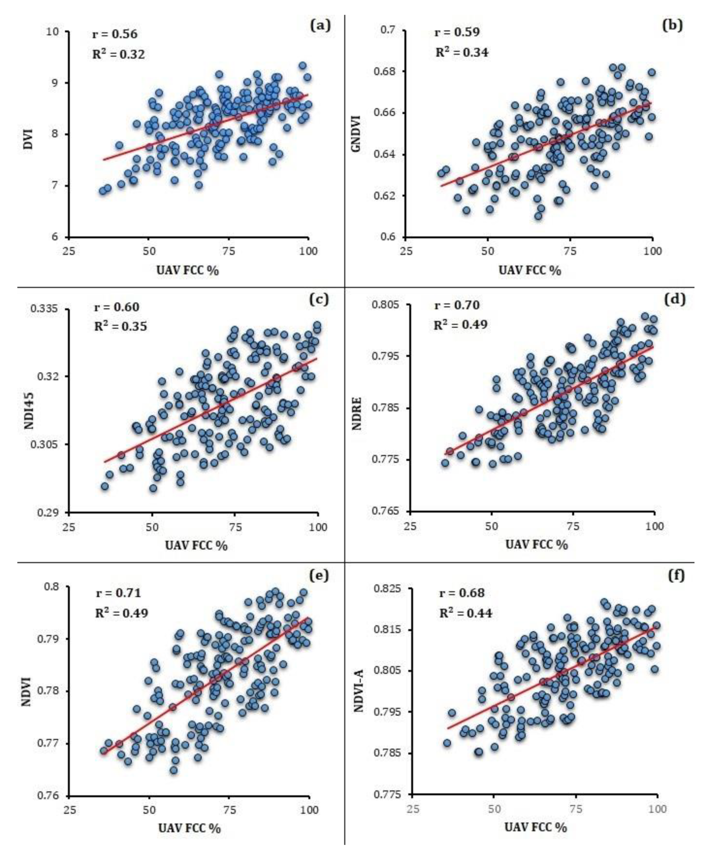
2.5. Relationship between FCC and Vegetation Indices

The linear regression and Pearson’s correlation coefficient were used to assess the relationship between FCC (%) obtained from UAV images and the vegetation indices of Sentinel-2 images. To this end, at first, all UAV-based FCC samples obtained via OBIA workflow (Section 2.3) were overlaid on the results of vegetation indices. Then, the mean value (e.g., mean NDVI) of each grid cell was extracted and used in regression and correlation analysis.

2.6. Model Building

This study applied four ML models to map and predict FCC based on UAV training samples and Sentinel-2 satellite imagery. These models were then used for further model training, identification of the most important predictor variables, and canopy cover estimation. The workflow of the study is shown in Figure 3.
At first, we applied a 10-fold cross-validation (CV) resampling to the training samples in order to reach the optimal tuning parameters. CV is a widely used resampling method that accurately estimates the prediction error of models and tunes model parameters [57,58]. In the k-fold cross-validation, the training samples are split into k folds. The first fold is considered a validation set, and the ML model is fitted on the remaining folds. This process is repeated k times, with different folds reserved for model evaluation [59]. For model building, four ML algorithms were examined. Modeling was carried out by means of the R programming language (Ver. 3.5.0) in the R Caret modeling interface [60], E1071, random forest, XGBoost, and elastic net packages. Moreover, the variable-importance evaluation function in the R Caret package was used to quantify the importance of Sentinel-2 multispectral bands and vegetation indices in various models, and the variable importance scores were scaled to a maximum value of 100 and a minimum value of 0. The variable importance is commonly estimated by the effect of each predictor on the squared error. The improvement value of each predictor is averaged over the entire ensemble to compute the overall importance value [61]. After the prediction, the relationship between predicted values and the test dataset was modeled by means of linear regression. To evaluate the accuracy of each model, the coefficient of determination (R2), root-mean-square error (RMSE), and mean absolute error (MAE) were calculated.

2.6.1. Tuning Parameters

In ML algorithms, tuning parameters play a determining role in producing high-accuracy results [35,58,59]. ML algorithms have been found to be affected by overfitting, so optimal hyperparameter tuning is required to achieve both low bias and low variance [62,63]. Various tuning steps and parameters can be used for each ML algorithm. A series of performance tests were run in the tuning process of each ML model, and the optimal parameters were selected based on the highest overall accuracy, as described in the following subsections.

2.6.2. Random Forest

Random forest (RF) is a powerful ensemble ML method developed by Breiman [64], based on a combination of decision trees. The RF algorithm learns from a randomly selected sample of the training samples [37,38,65]. The samples are generated using bootstrapping, which means that some samples will be used several times in a single tree. After constructing the decision trees, the prediction result from each decision tree is generated. The RF algorithm determines the outcome according to the decision trees and voting results [64]. Two tuning parameters need to be set up in order to use the RF: the number of trees (ntree), and the number of features in each split (mtry) [37,64]. We tested and evaluated different ranges of ntree and mtry parameters in order to determine the best RF model for classification: ntree = 100, 200, 500, and 1000; mtry = 1:10, with a step size of 1, as suggested by Thanh Noi and Kappas [37].

2.6.3. Support Vector Machine

Support-vector machine (SVM) is a supervised learning model that analyzes data for classification and regression analysis through associated learning algorithms. Based on a user-defined kernel function, SVM transforms the original feature space into an N-dimensional space, and then seeks a hyperplane that enables classes to be separated [65]. In this study, we used the radial basis function (RBF) kernel of the SVM classifier, as past research in environmental sciences suggests that RBF is widely used for classification problems and shows a high prediction accuracy, e.g., [37,66]. An SVM classifier with an RBF kernel needs to be applied with two kernel parameters: cost (C), and kernel width (sigma) [61,67]. C determines the size of misclassification allowed in non-separable training data, enabling adjustment of the complexity of the training data (i.e., large C = more flexible model; small C = stiffened model) [67,68]. The sigma parameter controls the smoothing of the class-dividing hyperplane. In this regard, SVM finds the samples (support vectors) from different classes, which are the closest to the hyperplane. Then, the distance (margin) between the hyperplane and the support vectors is computed. SVM learns the projection into a higher dimensional space from the training dataset, where two or more classes can be separated by a hyperplane that maximizes the margin. The final classification is made based on the side of the hyperplane on which the unlabeled samples fall [69].

2.6.4. Extreme Gradient Boosting

Extreme gradient boosting (XGBoost) is a widely used gradient-boosting technique that has been found to provide improved efficiency and speed in tree-based (sequential decision trees) ML algorithms [70]. XGBoost focuses exclusively on decision trees as base classifiers, and minimizes the loss function so that it builds an additive expansion of the objective function. This technique reduces the computational complexity for finding the best split, which is the most time-consuming part of decision tree construction algorithms. In a split-finding algorithm, all possible splits are enumerated, and the candidate with the highest gain is selected [71]. XGBoost includes some tuning to refine the model [72]. The typical tuning parameters of the XGBoost model include the number of boosting iterations (nrounds), max tree depth (max_depth), shrinkage (eta), minimum loss reduction (gamma), and subsample ratio of columns (colsample_bytree) [61]. In this study, we used the Bayesian optimization algorithm to tune the hyperparameters of the XGBoost model, due to its fast running speed and low number of iterations [72,73].

2.6.5. Elastic Net

A critique of lasso regression led to the development of the elastic net algorithm (ENET) [74]. Lasso regression has the disadvantage that its variables can be too dependent on data and, therefore, unstable. The lasso function can be modified to include additional costs for a model with large coefficients, in order to address the stability problem of regression models [73,75]. In this regard, ENET uses two penalties (L1 and L2) to minimize the size of all coefficients during the training [68]. The L1 penalty (i.e., the lasso model) reduces the size of all coefficients, and allows some coefficients to be minimized down to zero, thereby removing the predictor from the model. As a consequence of the L2 penalty (i.e., ridge regression), all coefficient sizes are reduced, but no coefficients can be removed from the model [76,77]. The ENET model requires two tuning parameters called alpha (α) and lambda (λ). Alpha controls the tradeoff between the ridge and the lasso. The overall strength of the ENET penalty is controlled by the lambda parameter [78].

3. Results

3.1. Relationships between FCC and Vegetation Indices

We used linear regression and Pearson’s correlation coefficient (r) to assess the relationships between canopy cover and vegetation indices. The results are shown in Table 5 and Figure 4. In Figure 4, there is clear evidence of a positive correlation between UAV-based FCC and the values of vegetation indices (i.e., DVI, GNDVI, NDI45, NDRE, NDVI, and NDVI-A) derived from Sentinel-2 data. Overall, NDVI showed the highest correlation coefficient (r = 0.71, R2 = 0.49) to the FCC%, followed by NDRE (r = 0.71, R2 = 0.49) and NDI45 (r = 0.60, R2 = 0.35).

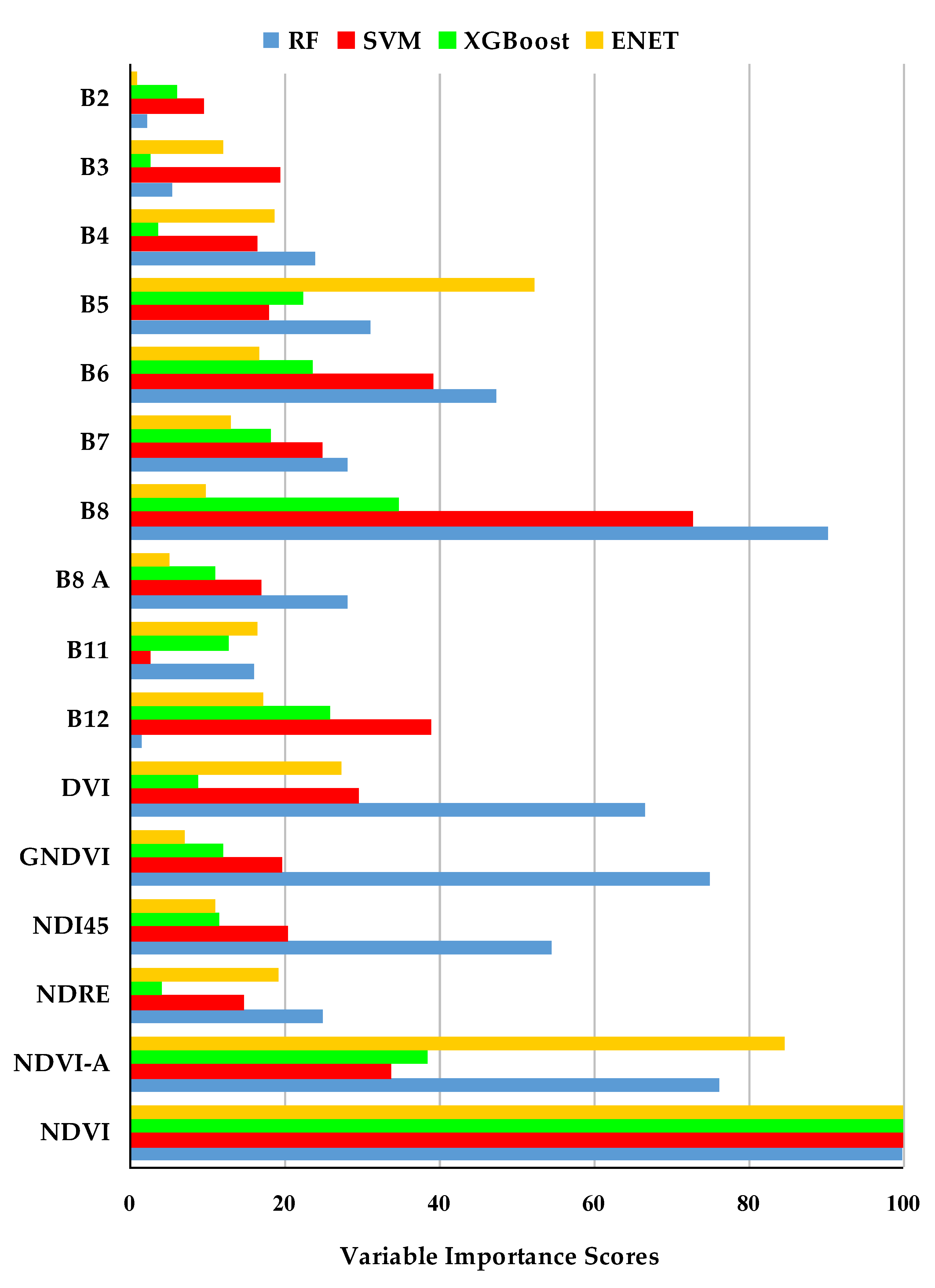
3.2. Variable Importance

The scores of the variable importance estimation are provided in Figure 5. Generally, the importance of variables for all of the used models (RF, SVM, XGBoost, and ENET) was similar, with NDVI, NDVI-A, NDRE, NDI45, and B8 (Sentinel-2 band 8) being the most important variables, followed by B6, B5, B12, DVI, and GNDVI (Figure 5).

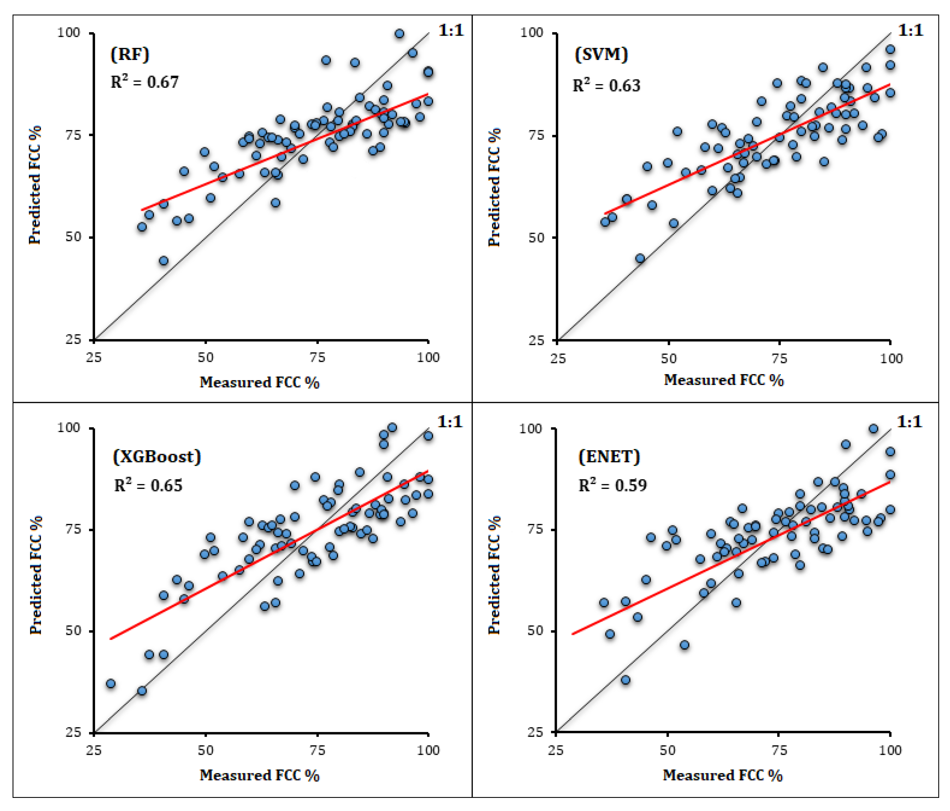
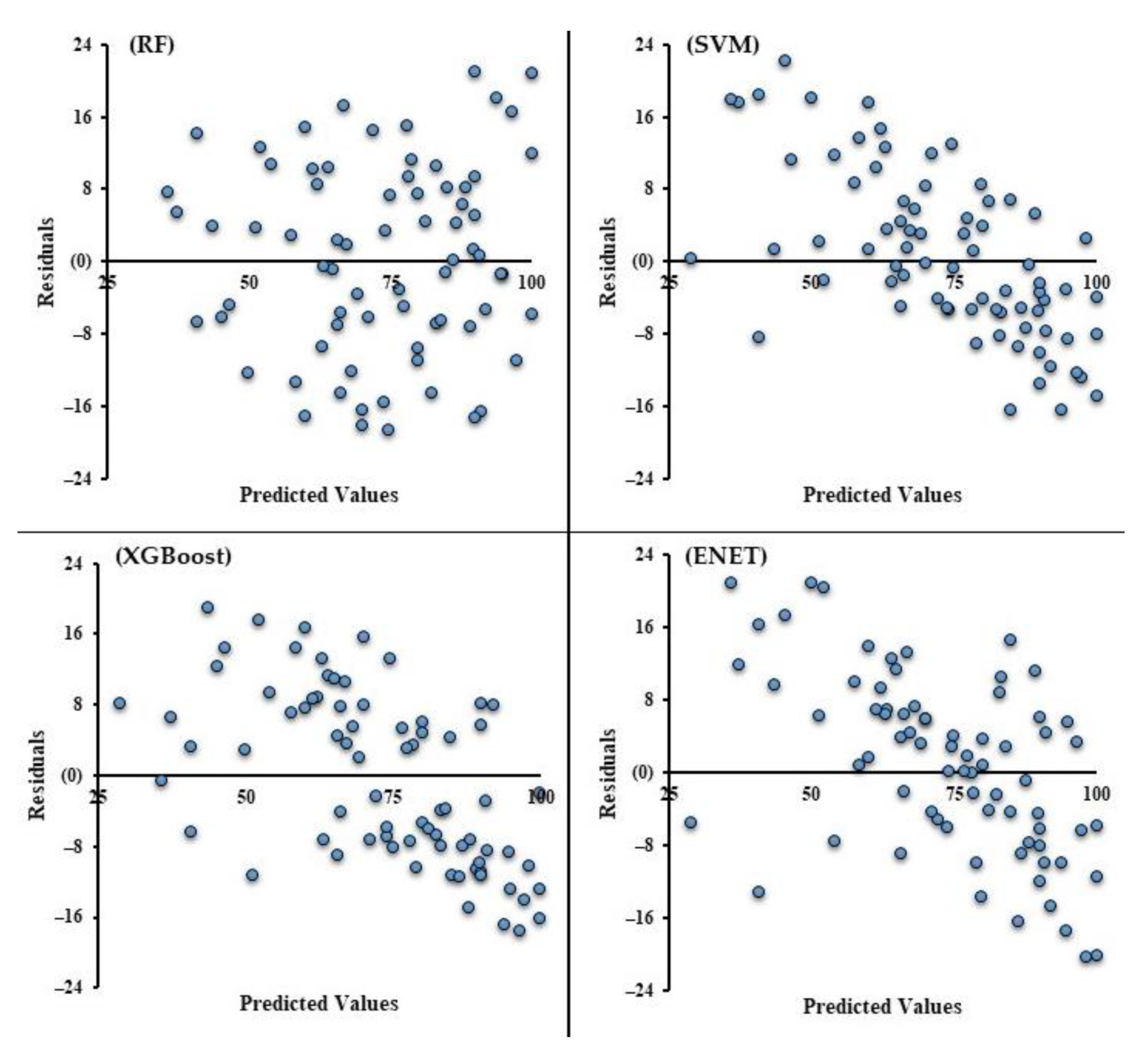
3.3. Comparison of ML Models

Model accuracy metrics including the R2, RMSE, MAE, and final (optimal) tuning parameters for each selected model are presented in Table 6. According to the results, the R2, RMSE, and MAE ranged from 0.59 to 0.67, 18.87 to 20.04%, and 15.34 to 16.44%, respectively. RF performed the best (R2 = 0.67, RMSE = 18.87%, MAE = 15.35%), and ENET the worst (R2 = 0.63, RMSE = 20.04%, MAE = 16.44%), among the tested ML models.
Scatterplots showing a comparison of the FCC values estimated by the ML models and the measured values (UAV-FCC) are given in Figure 6. We used a y = x straight line (i.e., 1:1 line) and the linear regression fitting line to better depict the positional relationships between the estimated and measured values. The main errors of the ML models were related to the overestimation of low-canopy-cover classes and underestimation of high-canopy-cover classes.
Residuals predicted by the ML models are shown in Figure 7. Based on the results, the residuals estimated by RF were found in a smaller range compared to those of other ML models. Additionally, the residual scatterplot of the RF model showed a rather random pattern, indicating that the RF model provided a decent fit to the data. The residuals predicted by the SVM, XGBoost, and ENET ML models showed similar distributions. According to the analysis of the residual scatterplots, there was an apparent overestimation of low FCC and an underestimation of high FCC, as returned by the SVM, XGBoost, and ENET ML models.
The RF model was then used to predict the FCC over the whole study site (Figure 8). The resulting FCC was reclassified into three classes: 1–30%, 31–60%, and 61–100%.

4. Discussion

The linear regression results between the UAV-based FCC and satellite-data-derived vegetation indices showed a strong positive correlation. ML evaluation of variable importance also confirmed these results. Vegetation indices, including NDVI, NDVI-A, NDRE, and NDI45, were the most important variables in our ML models. The NDVI and NDVI-A vegetation indices are based on the normalized difference between the NIR and red channels. Based on the work of Zhi-Hui et al. [79], normalized vegetation indices could eliminate the effects of solar height angle, satellite observation angle, topographic effect, cloud/shadow, and atmospheric attenuation; meanwhile, they reflect the canopy cover attributes. Previous studies also obtained similar results; for example, NDVI plays an essential role in predicting canopy density based on the vegetation indices derived from MODIS [25,80]. In addition to the common vegetation indices, our results confirmed the feasibility and high performance of red-edge band vegetation indices for canopy cover estimation. In our study, the NDRE and NDI45 indices were also found to be the dominant choices for ML models. NDRE and NDI45 are simple ratio indices that are very sensitive to canopy chlorophyll content. Studies have shown that the NDRE and NDI45 indices are significant predictors of canopy attributes [81,82]. Ali et al. [39] reported that the simple ratio vegetation indices based on the red-edge and NIR regions showed good performance for mapping canopy chlorophyll content. However, many factors may affect FCC modeling based on vegetation indices, which are commonly influenced by forest health, tree biomass, foliage density, chlorophyll content, and water stress. Halperin et al. [83] reported that SAVI and MSAVI are the most important variables in FCC estimation in low-canopy-cover forests, where the spectral signature may be affected by the soil background. In this study, Sentinel-2 multispectral bands, along with NIR, SWIR, and red-edge bands, played an important role in ML modeling. Therefore, the results confirm that Sentinel-2 spectral bands and the resultant vegetation indices are suitable tools for tree canopy cover modeling and mapping.
In this study, four ML models (i.e., RF, SVM, XGBoost, and ENET) with varying degrees of complexity were evaluated. The results obtained by the models were all indicative of a reasonable performance. Compared to the worst model (i.e., the ENET model; RMSE = 20.04%; R2 = 0.59), the RF model (RMSE = 18.87%; R2 = 0.67) slightly increased the prediction accuracy (a decrease in RMSE of 1.17% and an increase in R2 of 0.08). The SVM, ENET, and XGBoost models showed different degrees of overestimation and underestimation for low- and high-canopy-cover classes, respectively. A similar pattern of overestimation and underestimation was obtained by Zhi-Hui et al. [79]; based on their results, the behavior of vegetation indices is related to the vegetation density. In a high-density vegetation class, vegetation indices were compacted; therefore, they underestimated the FCC, and vice versa for a low-density vegetation class. Accordingly, overestimation and underestimation may be observed in forests with high heterogeneity in terms of canopy cover density. Given the findings, the RF is an effective model for FCC estimation, and can balance the problems of overestimation and underestimation. We assume that the overestimation or underestimation of FCC could depend on the FCC ranges or FCC values of training samples. This study was conducted in a dense forest, where most of our training samples used in ML modeling were collected for the dense class (FCC > 50%). Therefore, future studies may be conducted to evaluate the effect of FCC density on the performance of ML predictive accuracy.
The findings from this study corroborate the hypothesis that the synergic use of UAV RGB images, Sentinel-2 data, and ML algorithms can provide a valuable tool for tree canopy cover mapping of dense forests at the landscape scale. The quality of the available ground-truth dataset is critical to developing well-performing ML models [84]. In previous studies, ground-truth datasets were obtained via direct or indirect measurement, but technological and logistical limitations constrained field measurements. This study used high-resolution RGB images acquired via UAV to create a high-resolution ground-truth map. Our research shows that UAV-acquired imagery could be used instead of traditional field measurement methods to collect large amounts of accurate ground-truth data—particularly in dense montane forests. In contrast to the advantages of UAV, this method can be associated with some challenges, including those related to UAV image acquisition and tree crown delineation. The most important issues that should be considered are (1) acquisition of UAV ground-truth images from a wider range of study sites across a given case study area, so as to incorporate the heterogeneity of tree canopy cover, and (2) utilization of the most powerful segmentation methods and UAV-based extracted features, such as DSM and canopy height model (CHM), to better delineate the tree crowns. In short, our study describes and provides a simple, fast, and large-scale FCC modeling and mapping possibility. Compared with the traditional ground-based canopy cover measurements, the presented method has obvious benefits, i.e., cost-effectiveness, time-saving, and especially the potential of updating FCC maps.
The retrieval of FCC from Sentinel-2 images presents some limitations, such as being restricted to cloud-free daylight conditions, capturing information primarily from the top of the canopy, and being sensitive to surface reflectance saturation in moderate-to-high vegetation cover [85]. The limitations mentioned above can be addressed by using radio detection and ranging (RADAR) images in future research. In addition, the present study was based on single snapshots of FCC at each flight site, providing relatively restricted insights into how forest canopy may change over time. On the other hand, long-term monitoring of FCC dynamics and ground monitoring of plant demographic changes are important to understanding forest dynamics [86]. Another potential problem that might have impacted accuracy is the defoliation and discoloration specific to unhealthy trees, which could have been incorrectly excluded from the canopy mask by an automatic classification based only on spectral indices from the visible spectrum [61].

5. Conclusions

UAV systems equipped with GNSS and digital cameras can provide high-spatial-resolution, repetitive data at lower operational costs compared to ground-based forest inventories, particularly in challenging conditions such as those of FCC and crown attribute measurements. Sentinel-2 provides high-temporal-resolution data, with short revisit intervals (10 and 5 days at the Equator with one and two satellites, respectively), supporting a rich spectral configuration and a medium spatial resolution. While the combined use of these two remote sensing platforms offers advantages to forest inventory, testing the ML algorithms to examine their training performance based on remotely sensed datasets and clarifying their efficiency in FCC modeling is a base requirement. The best ML model could be further employed to generate large-scale FCC maps and to detect changes in forest canopy cover for given timelines. This study presented a methodological approach for FCC modeling in the Hyrcanian mixed temperate forests based on UAV-collected RGB imagery, Sentinel-2 imagery, and ML. The results obtained illustrate the suitability of integrating the UAV high-resolution aerial images, Sentinel-2 data, and ML models to estimate the FCC density in applications intended for precise and fast mapping of large forested areas.

Author Contributions

Conceptualization, V.N., A.A.D., H.A., and S.M.M.S.; data curation, V.N. and H.A.; formal analysis, V.N., and H.A.; funding acquisition, S.A.B.; investigation, V.N.; methodology, V.N. and V.C.G.; resources, V.N. and H.A.; software, V.N.; supervision, A.A.D. and H.A.; validation, V.N.; visualization, V.N.; writing—original draft preparation, V.N.; writing—review and editing, V.C.G., S.M.M.S., and S.A.B. All authors have read and agreed to the published version of the manuscript.

Funding

This research received no external funding, and the APC was funded by the Department of Forest Engineering, Forest Management Planning, and Terrestrial Measurements.

Institutional Review Board Statement

Not applicable.

Informed Consent Statement

Not applicable.

Data Availability Statement

The data supporting the findings of this study are available from the first author (V.N.), upon reasonable request.

Acknowledgments

We gratefully acknowledge Kheyrud Experimental Forest (Ehsan Abdi; University of Tehran) for his valuable support in the field investigation. This paper is a part of Vahid Nasiri’s doctoral thesis at the University of Tehran. Seyed Mohammad Moein Sadeghi’s research at the Transilvania University of Brasov, Romania, is supported by the program “Transilvania Fellowship for Postdoctoral Research/Young Researchers.” The authors acknowledge the support of the Department of Forest Engineering, Forest Management Planning, and Terrestrial Measurements, Faculty of Silviculture and Forest Engineering, Transilvania University of Brasov.

Conflicts of Interest

The authors declare no conflict of interest.

References

  1. Deljouei, A.; Sadeghi, S.M.M.; Abdi, E.; Bernhardt-Römermann, M.; Pascoe, E.L.; Marcantonio, M. The Impact of Road Disturbance on Vegetation and Soil Properties in a Beech Stand, Hyrcanian Forest. Eur. J. For. Res. 2018, 137, 759–770. [Google Scholar] [CrossRef]
  2. Pyngrope, O.R.; Kumar, M.; Pebam, R.; Singh, S.K.; Kundu, A.; Lal, D. Investigating Forest Fragmentation Through Earth Observation Datasets and Metric Analysis in the Tropical Rainforest Area. SN Appl. Sci. 2021, 3, 705. [Google Scholar] [CrossRef]
  3. Sadeghi, S.M.M.; Van Stan, J.T.; Pypker, T.G.; Tamjidi, J.; Friesen, J.; Farahnaklangroudi, M. Importance of Transitional Leaf States in Canopy Rainfall Partitioning Dynamics. Eur. J. For. Res. 2018, 137, 121–130. [Google Scholar] [CrossRef]
  4. Sadeghi, S.M.M.; Van Stan, J.T., II; Pypker, T.G.; Friesen, J. Canopy Hydrometeorological Dynamics Across a Chronosequence of A Globally Invasive Species, Ailanthus altissima (Mill., Tree of Heaven). Agric. For. Meteorol. 2017, 240, 10–17. [Google Scholar] [CrossRef]
  5. Korhonen, L.; Korhonen, K.T.; Rautiainen, M.; Stenberg, P.T. Estimation of Forest Canopy Cover: A Comparison of Field Measurement Techniques. Silva Fenn. 2006, 40, 577–588. [Google Scholar] [CrossRef] [Green Version]
  6. Gray, A.N.; McIntosh, A.C.; Garman, S.L.; Shettles, M.A. Predicting Canopy Cover of Diverse Forest Types from Individual Tree Measurements. For. Ecol. Manag. 2021, 501, 119682. [Google Scholar] [CrossRef]
  7. Imaizumi, F.; Nishii, R.; Ueno, K.; Kurobe, K. Forest Harvesting Impacts on Microclimate Conditions and Sediment Transport Activities in a Humid Periglacial Environment. Hydrol. Earth Syst. Sci. 2019, 23, 155–170. [Google Scholar] [CrossRef] [Green Version]
  8. Sadeghi, S.M.M.; Gordon, D.A.; Van Stan, J.T., II. A Global Synthesis of Throughfall and Stemflow Hydrometeorology. In Precipitation Partitioning by Vegetation; Springer: Cham, Switzerland, 2020; pp. 49–70. [Google Scholar]
  9. Chopping, M.; North, M.; Chen, J.Q.; Schaaf, C.B.; Blair, J.B.; Martonchik, J.V.; Bull, M.A. Forest Canopy Cover and Height from MISR in Topographically Complex Southwestern US Landscapes Assessed with High Quality Reference Data. IEEE J. Sel. Top. Appl. Earth Obs. Remote Sens. 2012, 5, 44–58. [Google Scholar] [CrossRef]
  10. Senf, C.; Sebald, J.; Seidl, R. Increasing Canopy Mortality Affects the Future Demographic Structure of Europe’s Forests. One Earth 2021, 4, 749–755. [Google Scholar] [CrossRef]
  11. Feldmann, E.; Drobler, L.; Hauck, M.; Kucbel, S.; Pichler, V.; Leuschner, C. Canopy Gap Dynamics and Tree Understory Release in a Virgin Beech Forest, Slovakian Carpathians. For. Ecol. Manag. 2018, 415, 38–46. [Google Scholar] [CrossRef]
  12. Rose, K.M.; Friday, J.B.; Oliet, J.A.; Jacobs, D.F. Canopy Openness Affects Microclimate and Performance of Underplanted Trees in Restoration of High-Elevation Tropical Pasturelands. Agric. For. Meteorol. 2020, 292, 108105. [Google Scholar] [CrossRef]
  13. Seidel, D.; Leuschner, C.; Scherber, C.; Beyer, F.; Wommelsdorf, T.; Cashman, M.J.; Fehrmann, L. The Relationship between Tree Species Richness, Canopy Space Exploration and Productivity in a Temperate Broad-Leaf Mixed Forest. For. Ecol. Manag. 2013, 310, 366–374. [Google Scholar] [CrossRef]
  14. Dormann, C.F.; Bagnara, M.; Boch, S.; Hinderling, J.; Janeiro-Otero, A.; Schäfer, D.; Schall, P.; Hartig, F. Plant Species Richness Increases with Light Availability, but not Variability, in Temperate Forests Understory. BMC Ecol. 2020, 43, 7411. [Google Scholar]
  15. Nakamura, A.; Kitching, R.L.; Cao, M.; Creedy, T.J.; Fayle, T.M.; Freiberg, M.; Hewitt, C.N.; Itioka, T.; Pin, K.L.; Ma, K.; et al. Forests and Their Canopies: Achievements and Horizons in Canopy Science. Trends Ecol. Evol. 2017, 32, 438–451. [Google Scholar] [CrossRef] [Green Version]
  16. Gastón, A.; Blázquez-Cabrera, S.; Mateo-Sánchez, M.C.; Simón, M.A.; Saura, S. The Role of Forest Canopy Cover in Habitat Selection: Insights from the Iberian lynx. Eur. J. Wildl. Res. 2019, 65, 30. [Google Scholar] [CrossRef]
  17. Erdody, T.L.; Moskal, L.M. Fusion of LiDAR and Imagery for Estimating Forest Canopy Fuels. Remote Sens. Environ. 2010, 114, 725–737. [Google Scholar] [CrossRef]
  18. Palaiologou, P.; Kalabokidis, K.; Ager, A.A.; Day, M.A. Development of Comprehensive Fuel Management Strategies for Reducing Wildfire Risk in Greece. Forests 2020, 11, 789. [Google Scholar] [CrossRef]
  19. Gill, S.J.; Biging, G.S.; Murphy, E.C. Modeling Conifer Tree Crown Radius and Estimating Canopy Cover. For. Ecol. Manag. 2000, 126, 405–416. [Google Scholar] [CrossRef] [Green Version]
  20. Mcintosh, A.C.; Gray, A.; German, S.L. Estimating Canopy Cover from Standard Forest Inventory Measurements in Western Oregon. For. Sci. 2012, 58, 154–167. [Google Scholar] [CrossRef] [Green Version]
  21. Bianchi, S.; Cahalan, C.; Hale, S.; Gibbons, J.M. Rapid Assessment of Forest Canopy and Light Regime Using Smartphone Hemispherical Photography. Ecol. Evol. 2017, 24, 10556–10566. [Google Scholar] [CrossRef] [Green Version]
  22. Brumelis, G.; Dauskane, I.; Elferts, D.; Strode, L.; Krama, T.; Kramas, I. Estimates of Tree Canopy Closure and Basal Area as Proxies for Tree Crown Volume at a Stand Scale. Forests 2020, 11, 1180. [Google Scholar] [CrossRef]
  23. Khokthong, W.; Zemp, D.C.; Irawan, B.; Sundawati, L.; Kreft, H.; Holscher, D. Drone-Based Assessment of Canopy Cover for Analyzing Tree Mortality in an Oil Palm Agroforest. Front. Glob. Chang. 2019, 2, 12. [Google Scholar] [CrossRef] [Green Version]
  24. Eskandari, S.; Jaafari, M.R.; Oliva, P.; Ghorbanzadeh, O.; Blaschke, T. Mapping Land Cover and Tree Canopy Cover in Zagros Forests of Iran: Application of Sentinel-2, Google Earth, and Field Data. Remote Sens. 2020, 12, 1912. [Google Scholar] [CrossRef]
  25. Huang, X.; Wu, W.; Shen, T.; Xie, L.; Qin, Y.; Peng, S.; Zhou, X.; Fu, X.; Li, J.; Zhang, Z.; et al. Estimating Forest Canopy Cover by Multiscale Remote Sensing in Northeast Jiangxi, China. Land 2021, 10, 433. [Google Scholar] [CrossRef]
  26. Miranda, A.; Catalán, G.; Altamirano, A.; Zamorano-Elgueta, C.; Cavieres, M.; Guerra, J.; Mola-Yudego, B. How Much Can We See from a UAV-Mounted Regular Camera? Remote Sensing-Based Estimation of Forest Attributes in South American Native Forests. Remote Sens. 2021, 13, 2151. [Google Scholar] [CrossRef]
  27. Devaney, J.; Barret, B.; Barrett, F.; Redmond, J. Forest Cover Estimation in Ireland Using Radar Remote Sensing: A Comparative Analysis of Forest Cover Assessment Methodologies. PLoS ONE 2015, 10, e0133583. [Google Scholar] [CrossRef] [Green Version]
  28. Anchang, J.; Prihodko, L.; Ji, W.; Kumar, S.S.; Ross, C.W.; Yu, Q.; Lind, B.; Sarr, M.A.; Diouf, A.A.; Hanan, N.P. Toward Operational Mapping of Woody Canopy Cover in Tropical Savannas Using Google Earth Engine. Front. Environ. Sci. 2020, 30, 4. [Google Scholar] [CrossRef] [Green Version]
  29. Ma, Q.; Su, Y.; Guo, Q. Comparison of Canopy Cover Estimations from Airborne LiDAR, Aerial Imagery, and Satellite Imagery. IEEE J. Sel. Top. Appl. Earth Obs. Remote Sens. 2017, 99, 4225–4236. [Google Scholar] [CrossRef]
  30. Lima, T.A.; Beuchle, R.; Langner, A.; Grecchi, R.C.; Griess, V.C.; Achard, F. Comparing Sentinel-2 MSI and Landsat 8 OLI Imagery for Monitoring Selective Logging in the Brazilian Amazon. Remote Sens. 2019, 11, 961. [Google Scholar] [CrossRef] [Green Version]
  31. Cortés-Molino, A.; Maestro, I.A.; Fernandez-Luque, I.; Flores-Moya, A.; Carreira, J.A.; Tierra, A.E.S. Using ForeStereo and LIDAR Data to Assess Fire and Canopy Structure-Related Risks in Relict Abies pinsapo Boiss. PeerJ 2020, 8, e10158. [Google Scholar] [CrossRef]
  32. Bagaram, M.B.; Giuliarelli, D.; Chirici, G.; Giannetti, F.; Barbati, A. UAV Remote Sensing for Biodiversity Monitoring: Are Forest Canopy Gaps Good Covariates? Remote Sens. 2018, 10, 1397. [Google Scholar]
  33. Karlson, M.; Ostwald, M.; Reese, H.; Sanou, J.; Boalidioa, T.; Mattsson, E. Mapping Tree Canopy Cover and Aboveground Biomass in Sudano-Sahelian Woodlands Using Landsat 8 and Random Forest. Remote Sens. 2015, 7, 10017–10041. [Google Scholar] [CrossRef] [Green Version]
  34. Jin, D.; Qi, J.; Huang, H.; Li, L. Combining 3D Radiative Transfer Model and Convolutional Neural Network to Accurately Estimate Forest Canopy Cover from Very High-Resolution Satellite Images. IEEE J. Sel. Top. Appl. Earth Obs. Remote Sens. 2021, 14, 10953–10963. [Google Scholar] [CrossRef]
  35. Ganz, S.; Adler, P.; Kandler, G. Forest Cover Mapping Based on a Combination of Aerial Images and Sentinel-2 Satellite Data Compared to National Forest Inventory Data. Forests 2020, 11, 1322. [Google Scholar] [CrossRef]
  36. Hua, Y.; Zhao, X. Multi-Model Estimation of Forest Canopy Closure by Using Red Edge Bands Based on Sentinel-2 Images. Forests 2021, 12, 1768. [Google Scholar] [CrossRef]
  37. Thanh Noi, P.; Kappas, M. Comparison of Random Forest, k-Nearest Neighbor, and Support Vector Machine Classifiers for Land Cover Classification Using Sentinel-2 Imagery. Sensors 2018, 18, 18. [Google Scholar] [CrossRef] [Green Version]
  38. Moradi, F.; Darvishsefat, A.A.; Pourrahmati, M.R.; Deljouei, A.; Borz, S.A. Estimating Aboveground Biomass in Dense Hyrcanian Forests by the Use of Sentinel-2 Data. Forests 2022, 13, 104. [Google Scholar] [CrossRef]
  39. Ali, A.M.; Darvishzadeh, R.; Skidmore, A.; Gara, T.W.; O’Connor, B.; Roeoesli, C.; Heurich, M.; Paganini, M. Comparing Methods for Mapping Canopy Chlorophyll Content in a Mixed Mountain Forest using Sentinel-2 Data. Int. J. Appl. Earth Obs. 2020, 87, 102037. [Google Scholar] [CrossRef]
  40. Su, M.; Guo, R.; Chen, B.; Hong, W.; Wang, J.; Feng, Y.; Xu, B. Sampling Strategy for Detailed Urban Land Use Classification: A Systematic Analysis in Shenzhen. Remote Sens. 2020, 12, 1497. [Google Scholar] [CrossRef]
  41. Bhandari, S.; Raheja, A.; Chaichi, M.R.; Green, R.L.; Do, D.; Ansari, M.; Pham, F.; Wolf, J.; Sherman, T.; Espinas, A. Ground-Truthing of UAV-Based Remote Sensing Data of Citrus Plants. In Proceedings of the Autonomous Air and Ground Sensing Systems for Agricultural Optimization and Phenotyping III, Orlando, FL, USA, 21 May 2018. [Google Scholar]
  42. Mazzia, V.; Comba, L.; Khaliq, A.; Chiaberge, M.; Gay, P. UAV and Machine Learning-Based Refinement of a Satellite-Driven Vegetation Index for Precision Agriculture. Sensors 2020, 20, 2530. [Google Scholar] [CrossRef]
  43. Nasiri, V.; Darvishsefat, A.A.; Arefi, H.; Pierrot-Deseilligny, M.; Namiranian, M.; Le-Bris, A. Unmanned Aerial Vehicles (UAV) Based Canopy Height Modeling Under Leaf-On and Leaf-Off Conditions for Determining Tree Height and Crown Diameter (Case Study: Hyrcanian Mixed Forest). Can. J. For. Res. 2021, 51, 962–971. [Google Scholar] [CrossRef]
  44. Torresan, C.; Carotenuto, F.; Chiavetta, U.; Miglietta, F.; Zaldei, A.; Gioli, B. Individual Tree Crown Segmentation in Two-Layered Dense Mixed Forests from UAV LiDAR Data. Drones 2020, 4, 10. [Google Scholar] [CrossRef] [Green Version]
  45. Yao, H.; Qin, R.; Chen, X. Unmanned Aerial Vehicle for Remote Sensing Applications—A Review. Remote Sens. 2019, 11, 1443. [Google Scholar] [CrossRef] [Green Version]
  46. Deljouei, A.; Abdi, E.; Schwarz, M.; Majnounian, B.; Sohrabi, H.; Dumroese, R.K. Mechanical Characteristics of the Fine Roots of Two Broadleaved Tree Species from the Temperate Caspian Hyrcanian Ecoregion. Forests 2020, 11, 345. [Google Scholar] [CrossRef] [Green Version]
  47. WHC. UNESCO World Heritage Centre. 2021. Available online: https://whc.unesco.org/en/list/1584 (accessed on 17 December 2021).
  48. Marvi Mohadjer, M.R. Silviculture; University of Tehran Press: Tehran, Iran, 2012; p. 387. [Google Scholar]
  49. Mészarós, J. Aerial Surveying UAV Based on Open-Source Hardware and Software. Int. Arch. Photogramm. Remote Sens. Spat. Inf. Sci. 2011, 37, 555. [Google Scholar] [CrossRef] [Green Version]
  50. eCognition. Trimble Geospatial. Available online: https://geospatial.trimble.com/products-and-solutions/ecognition (accessed on 17 December 2020).
  51. Main-Knorn, M.; Pflug, B.; Louis, J.; Debaecker, V.; Muller-Wilm, U.; Gascon, F. Sen2Cor for Sentinel-2. Proc. SPIE 2017, 10427, 1–12. [Google Scholar] [CrossRef] [Green Version]
  52. Raiyani, K.; Gonçalves, T.; Rato, L.; Salgueiro, P.; Marques da Silva, J.R. Sentinel-2 Image Scene Classification: A Comparison Between Sen2Cor and a Machine Learning Approach. Remote Sens. 2021, 13, 300. [Google Scholar] [CrossRef]
  53. STEP Science Toolbox Exploitation Platform (SNAP). Available online: http://step.esa.int/main/toolboxes/snap (accessed on 17 December 2020).
  54. Zhao, L.; Dai, A.; Dong, B. Changes in Global Vegetation Activity and its Driving Factors during 1982–2013. Agric. For. Meteorol. 2018, 249, 198–209. [Google Scholar] [CrossRef]
  55. Qi, H.; Chehbouni, A.; Huete, A.R.; Kerr, Y.H.; Sorooshian, S. A Modified Soil Adjusted Vegetation Index. Remote Sens. Environ. 1994, 48, 119–126. [Google Scholar] [CrossRef]
  56. Guyot, G.; Baret, F. Spectral Signatures of Objects in Remote Sensing. In Proceedings of the International Colloquium Spectral Signatures of Objects in Remote Sensing, Aussois Modane, France, 18–22 January 1988. [Google Scholar]
  57. Berrar, D. Cross Validation. J. Bioinform. Comput. Biol. 2018, 1, 542–545. [Google Scholar]
  58. Karadal, C.H.; Kaya, M.C.; Tuncer, T.; Dogan, S.; Acharya, U.R. Automated Classification of Remote Sensing Images Using Multileveled MobileNetV2 and DWT Techniques. Expert Syst. Appl. 2021, 185, 115659. [Google Scholar] [CrossRef]
  59. Ramezan, C.A.; Warner, T.A.; Maxwell, A.E. Evaluation of Sampling and Cross-Validation Tuning Strategies for Regional-Scale Machine Learning Classification. Remote Sens. 2019, 11, 185. [Google Scholar] [CrossRef] [Green Version]
  60. Kuhn, M. Building Predictive Models in R Using the Caret Package. J. Stat. Softw. 2008, 28, 1–26. [Google Scholar] [CrossRef] [Green Version]
  61. Pilaš, I.; Gašparović, M.; Novkinić, A.; Klobučar, D. Mapping of the Canopy Openings in Mixed Beech–Fir Forest at Sentinel-2 Subpixel Level Using UAV and Machine Learning Approach. Remote Sens. 2020, 12, 3925. [Google Scholar] [CrossRef]
  62. He, M.; Xu, Y.; Li, N. Population Spatialization in Beijing City Based on Machine Learning and Multisource Remote Sensing Data. Remote Sens. 2020, 12, 1910. [Google Scholar] [CrossRef]
  63. Ghatkar, J.G.; Singh, R.K.; Shanmugam, P. Classification of Algal Bloom Species from Remote Sensing Data Using an Extreme Gradient Boosted Decision Tree Model. Int. J. Remote Sens. 2019, 40, 9412–9438. [Google Scholar] [CrossRef]
  64. Breiman, L. Random Forests. Mach. Learn. 2001, 45, 5–32. [Google Scholar] [CrossRef] [Green Version]
  65. Misra, S.; Li, H.; He, J. Machine Learning for Subsurface Characterization; Gulf Professional Publishing: Cambridge, MA, USA, 2019. [Google Scholar]
  66. Gomroki, M.; Jafari, M.; Sadeghian, S.; Azizi, Z. Application of Intelligent Interpolation Methods for DTM Generation of Forest Areas based on Lidar Data. J. Photogramm. Remote Sensi. Geoinform. Sci. 2017, 85, 227–241. [Google Scholar] [CrossRef]
  67. Ballanti, L.; Blesius, L.; Hines, E.; Kruse, B. Tree Species Classification Using Hyperspectral Imagery: A Comparison of Two Classifiers. Remote Sens. 2016, 8, 445. [Google Scholar] [CrossRef] [Green Version]
  68. Wang, M.; Wan, Y.; Ye, Z.; Lai, X. Remote Sensing Image Classification Based on the Optimal Support Vector Machine and Modified Binary Coded ant Colony Optimization Algorithm. Inf. Sci. 2017, 402, 50–68. [Google Scholar] [CrossRef]
  69. Evgeniou, T.; Pontil, M. Support Vector Machines: Theory and Applications. In Advanced Course on Artificial Intelligence (ACAI); Springer: Berlin/Heidelberg, Germany, 2001. [Google Scholar]
  70. Chen, T.; Guestrin, C. XGBoost: A Scalable Tree Boosting System. In Proceedings of the 22nd ACM SIGKDD International Conference on Knowledge Discovery and Data, San Francisco, CA, USA, 13–17 August 2016. [Google Scholar]
  71. Bentejac, C.; Csorgo, A.; Martinez-Munoz, G. A Comparative Analysis of Gradient Boosting Algorithms. Artif. Intell. Rev. 2021, 54, 1937–1967. [Google Scholar] [CrossRef]
  72. Su, H.; Yang, X.; Lu, W.; Yan, X.H. Estimating Subsurface Thermohaline Structure of the Global Ocean Using Surface Remote Sensing Observations. Remote Sens. 2019, 11, 1598. [Google Scholar] [CrossRef] [Green Version]
  73. Yang, X.; Yang, R.; Ye, Y.; Yuan, Z.; Wang, D.; Hua, K. Winter wheat SPAD Estimation from UAV Hyperspectral Data Using Cluster-Regression Methods. Int. J. Appl. Earth Obs. Geoinf. 2021, 105, 102618. [Google Scholar] [CrossRef]
  74. Zou, H.; Hastie, T. Regularization and Variable Selection via the Elastic Net. J. R. Stat. Soc. 2005, 67, 301–320. [Google Scholar] [CrossRef] [Green Version]
  75. Hong, Y.; Chen, Y.; Yu, L.; Liu, Y.; Liu, Y.; Zhang, Y.; Liu, Y.; Cheng, H. Combining Fractional Order Derivative and Spectral Variable Selection for Organic Matter Estimation of Homogeneous Soil Samples by VIS–NIR Spectroscopy. Remote Sens. 2018, 10, 479. [Google Scholar] [CrossRef] [Green Version]
  76. El Anbari, E.M.; Mkhadri, A. Penalized Regression with a Combination of the L1 Norm and the Correlation-Based Penalty. Ph.D. Thesis, The National Institute for Research in Digital Science and Technology (INRIA), Le Chesnay-Rocquencourt, France, 2009. [Google Scholar]
  77. Zhao, Y.L.; Feng, Y.L. Learning Performance of Elastic-Net Regularization. Math. Comput. Model. 2013, 57, 1395–1407. [Google Scholar] [CrossRef]
  78. Kim, K.; Koo, J.; Sun, H. An Empirical Threshold of Selection Probability for Analysis of High-Dimensional Correlated Data. J. Stat. Comput. Simul. 2020, 90, 1606–1617. [Google Scholar] [CrossRef]
  79. Zhi-Hui, M.; Lei, D.; Fu-Zhou, D.; Xiao-Juan, L.; Dan-Yu, Q. Angle Effects of Vegetation Indices and the Influence on Prediction of SPAD Values in Soybean and Maize. Int. J. Appl. Earth. Obs. 2020, 94, 102198. [Google Scholar]
  80. Tsalyuk, M.; Kelly, M.; Getz, W.M. Improving the Prediction of African Savanna Vegetation Variables Using Time Series of MODIS Products. ISPRS J. Photogramm. Remote Sens. 2017, 131, 77–91. [Google Scholar] [CrossRef] [Green Version]
  81. Wang, Z.; Wang, T.; Darvishzadeh, R.; Skidmore, A.; Jones, S.; Suarez, L.; Woodgate, W.; Heiden, U.; Heurich, M.; Hearne, J. Vegetation Indices for Mapping Canopy Foliar Nitrogen in a Mixed Temperate Forest. Remote Sens. 2016, 8, 491. [Google Scholar] [CrossRef] [Green Version]
  82. Zimmermann, S.; Hoffmann, K. Evaluating the Capabilities of Sentinel-2 Data for Large-Area Detection of Bark Beetle Infestation in the Central German Uplands. J. Appl. Remote. Sens. 2020, 14, 24515. [Google Scholar] [CrossRef]
  83. Halperin, J.; Lemay, V.; Chidumayo, E.; Verchot, L.; Marshall, P. Model-Based Estimation of Above-Ground Biomass in the Miombo Ecoregion of Zambia. For. Ecosyst. 2016, 3, 14. [Google Scholar] [CrossRef] [Green Version]
  84. Hegarty-Craver, M.; Polly, J.; O’Neil, M.; Ujeneza, N.; Rineer, J.; Beach, R.H.; Lapidus, D.; Temple, D. Remote Crop Mapping at Scale: Using Satellite Imagery and UAV-Acquired Data as Ground Truth. Remote Sens. 2020, 12, 1984. [Google Scholar] [CrossRef]
  85. Wang, J.; Xiao, X.; Bajgain, R.; Starks, P.; Steiner, J.; Doughty, R.B.; Chang, Q. Estimating Leaf Area Index and Aboveground Biomass of Grazing Pastures Using Sentinel-1, Sentinel-2 and Landsat Images. ISPRS J. Photogramm. Remote Sens. 2019, 154, 189–201. [Google Scholar] [CrossRef] [Green Version]
  86. Davies, S.J.; Abiem, I.; Salim, K.A.; Aguilar, S.; Allen, D.; Alonso, A.; Anderson-Teixeira, K.; Andrade, A.; Arellano, G.; Ashton, P.S.; et al. ForestGEO: Understanding Forest Diversity and Dynamics Through a Global Observatory Network. Biol. Conserv. 2021, 253, 108907. [Google Scholar] [CrossRef]
Figure 1. Location of the study area and the ground-truth map based on unmanned aerial vehicle (UAV) true color RGB images.
Remotesensing 14 01453 g001
Figure 2. Ground-truth map generated from the unmanned aerial vehicle (UAV) data: (a) Image segmentation using the multiresolution segmentation (MRS) method to determine tree crown borders. (b) Classification of segmented images as tree crowns or canopy gaps. (c) The resulting map of forest canopy cover percentage (FCC%).
Remotesensing 14 01453 g002
Figure 3. Experimental design of the forest canopy cover (FCC) prediction.
Remotesensing 14 01453 g003
Figure 4. Linear relationships between UAV-based forest canopy cover percentage (FCC%) and vegetation indices: (a) DVI = difference vegetation index; (b) GNDVI = green normalized difference vegetation index; (c) NDI45 = normalized difference index 4 and 5 red edge; (d) NDRE = normalized difference red-edge index; (e) NDVI = normalized difference vegetation index; (f) NDVI-A = normalized difference vegetation index based on B8 A.
Remotesensing 14 01453 g004
Figure 5. Variable importance scores for Sentinel-2 multispectral bands and vegetation indices.
Remotesensing 14 01453 g005
Figure 6. Scatterplots of measured and predicted forest canopy cover percentage (FCC%) values.
Remotesensing 14 01453 g006
Figure 7. Residual scatterplots of predicted forest canopy cover percentage (FCC%) by the tested machine learning models.
Remotesensing 14 01453 g007
Figure 8. The forest canopy cover percentage (FCC%) map derived from using the random forest (RF) algorithm on the Sentinel-2 data.
Remotesensing 14 01453 g008
Table 1. Descriptive statistics of the unmanned aerial vehicle (UAV) missions and data processing workflow.
InformationUAV Mission
1234
Area (ha)20151719
Flight Altitude (m)100100100100
Number of Images276170193260
Aligned Images260158170257
Side and Forward Overlap (%)80808080
Number of GCPs4444
Georeferencing Errors
X Error (cm)2.23.61.91.3
Y Error (cm)0.82.11.80.7
Z Error (cm)0.42.61.21.3
Total Error (cm)1.42.12.21.8
GNSS Measurement Errors
Number of GCPs4444
Minimum of XY Error (cm)11.18.45.59.7
Maximum of XY Error (cm)13.111.58.412.2
Minimum of Z Error (cm)10.69.99.110.6
Maximum of Z Error (cm)17.212.59.714.5
Table 2. Parameters used in the photogrammetric workflow.
Processing StepParameter NameParameter Value
Aligning ImagesAccuracyHighest
Optimization of Image AlignmentDefaultf, b1, b2, cx, cy, k1, k2, p1, and p2
The Ground Control Point Placement Manual
Building Dense PointsQualityHigh
Mesh BuildingSurface typeHeight field
Source dataDense points
Face countHigh
OrthomosaicBlending modeMosaic
Coordinate systemWGS 84/UTM
Table 3. Characteristics and technical specifications of the UAV.
CharacteristicsTechnical Specifications
Diagonal Wheelbase105 cm
Size of Propeller38 cm
Length of One Arm42 cm
Net Weight2.25 kg
Battery(2×) 6S, 16,000 mHA
NavigationManual/automatic
CommunicationAntenna tracking systems
Resolution of RGB Camera12 megapixel
Resolution of IR Camera12 megapixel
Practical Range4 km
Operational Altitude50 to 300 m
Takeoff Weight10 kg
Total Weight9 kg
Flight Duration30 min
Table 4. Vegetation indices used for forest canopy cover (FCC) modeling.
Vegetation IndexSpectral BandsSentinel-2 FormulaReferences
DVIRed, NIRB8/B4[54,55,56]
NDVIRed, NIRB8-B4/B8 + B4
NDVI2Red, NIRB8a-B4/B8 A + B4
GNDVIGreen, NIRB8-B3/B8 + B3
NDI45Red, red edgeB5-B4/B5 + B4
NDRERed edge, NIRB8-B5/B8 + B5
Note: DVI = difference vegetation index; NDVI = normalized difference vegetation index; GNDVI = green normalized difference vegetation index; NDI45 = normalized difference index 4 and 5 red edge; NDRE = normalized difference red edge index.
Table 5. Correlation between the forest canopy cover percentage (FCC%) and vegetation indices (n = 240).
Vegetation IndicesDVIGNDVINDI45NDRENDVINDVI-A
Pearson Correlation (r)0.560.590.600.700.710.68
Coefficient of Determination (R2)0.320.340.350.490.490.44
Table 6. Comparison of the performance of different machine learning models.
AlgorithmR2RMSE (%)MAE (%)Tuning Parameters
RF0.6718.8715.35mtry = 9; ntree = 1000
SVM0.6319.2415.55C = 1; Sigma = 0.0950
XGBoost0.6519.0515.45nrounds = 50; max_depth = 3; eta = 0.3; Gamma = 0; colsample_bytree = 0.8
ENET0.5920.0416.44Alpha = 0.4; Lambda = 0.04
Publisher’s Note: MDPI stays neutral with regard to jurisdictional claims in published maps and institutional affiliations.

