Diversity Effects on Canopy Structure Change throughout a Growing Season in Experimental Grassland Communities

Abstract

Increasing plant diversity commonly enhances standing biomass and other ecosystem functions (i.e., carbon fluxes, water use efficiency, herbivory). The standing biomass is correlated with vegetation volume, which describes plant biomass allocation within a complex canopy structure. As the canopy structure of plant communities is not static throughout time, it is expected that its changes also control diversity effects on ecosystem functioning. Yet, most studies are based on one or two measures of ecosystem function per year. Here, we examine the temporal effects of diversity of grassland communities on canopy structural components in high temporal (bi-weekly throughout the growing season) and spatial resolutions as a proxy for ecosystem functioning. Using terrestrial laser scanning, we estimate metrics of vertical structure, such as biomass distribution (evenness) and highest biomass allocation (center of gravity) along height strata. For horizontal metrics, we calculated community stand gaps and canopy surface variation. Our findings show that species-rich communities start filling the vertical space (evenness) earlier in the growing season, suggesting a more extended period of resource use (i.e., light-harvesting). Moreover, more diverse communities raised their center of gravity only at the peak of biomass in spring, likely triggered by higher interspecific competition inducing higher biomass allocation at upper layers of the canopy. Furthermore, richer communities were clumpier only after mowing, revealing species-specific differences in regrowth. Lastly, species richness strongly affected canopy variation when the phenology status and height differences were maximal, suggesting differences in plant functional strategies (space to grow, resource use, and flowering phenology). Therefore, the effects of diversity on ecosystem functions depending on those structural components such as biomass production, decomposition, and herbivory, may also change throughout the season due to various mechanisms, such as niche differences, increased complementarity, and temporal and spatial variation in biological activity.

1. Introduction

Compelling evidence shows that biodiversity enhances ecosystem functioning—an effect best studied for plant community biomass [1,2,3,4,5]. Standing biomass has been shown to be directly correlated to the volume of vegetation, which was recently successfully estimated using terrestrial laser scanning techniques [6,7,8], as well as shown to be positively correlated with plant height (a basis for volume calculation) also using the same technique [9]. Within a given volume of vegetation, differing plant biomass allocation patterns may create complex canopy structures with variations in height and density of different plant organs such as leaves, stems, and flowers. These patterns in canopy structure can change with plant species richness and exhibit characteristic spatial (i.e., biomass distribution along vertical or horizontal profiles) [10] and temporal patterns (i.e., seasonal variation of canopy height) [11,12]. Given that light capture and downstream processes related to photosynthesis strongly depend on where leaf biomass is allocated within the canopy [13], an optimal distribution of canopy structural components may be an important prerequisite of complementarity in light use in more diverse vegetation [14,15,16,17]. Therefore, a precise characterization of the canopy structure has the potential to elucidate underlying mechanisms of biodiversity–ecosystem functioning relationships [10,18]. However, which components of canopy structure relate to plant diversity and how these relationships change throughout the growing season in grassland communities still merits thorough investigation. Here, we study the phenology of canopy components with high spatial and temporal resolution in dynamic, managed grassland communities.

Previous studies have shown that coarse measures of plant community structural components like canopy height, vegetation density, and the vertical distribution of biomass could drive plant diversity effects on different ecosystem functions. For instance, positive effects of biodiversity on plant biomass were associated with diverse mixtures attaining taller canopy heights in grassland plant communities [9,13,19,20] and forests [21,22]. Moreover, increasing vegetation density triggers an asymmetric competition for the light, driving higher biomass with increasing plant diversity in grasslands [18,23]. Variation in plant height (represented by vertical stratification of the plant canopy) also mediated positive effects of plant diversity on habitat provision quantified as arthropod abundance in forests and on arthropod species richness in grasslands ecosystems [10]. In addition, a study on the abundance and richness of carnivorous arthropods showed their positive association with diverse plant communities via increased canopy space-filling by small-statured forbs [24]. Overall, these findings suggest that investigating determinants of canopy structure could advance our mechanistic understanding of biodiversity–ecosystem functioning relationships. However, so far, we lack information on quantitative measures of canopy structural components in grassland communities concerning plant species richness and, in particular, their spatial and temporal changes. As canopy structural components are not static but change over time (here we consider changes throughout the growing season), one can expect a change in the strength and direction of their impact on the biodiversity–ecosystem functioning relationship over time. Even though grassland ecosystems are highly dynamic [25,26,27], most of the studies in grasslands focus on the peak of biomass and therefore do not reflect and integrate over seasonal changes in the canopy structural components and their diversity signature.

Temporal variability in Central European grasslands is induced by species-specific asynchrony in phenology and modified by species interactions [28,29]. Grassland species exhibit distinct activity periods of plants throughout the growing season and management regimes (e.g., mowing or grazing), leading to seasonal changes in vegetation structure. Canopy structural components (volume, height, density) reflect the spatial heterogeneity of vegetation in terms of overall volume and vertical and horizontal architecture of plant community stands and how these structures change throughout sward development [30]. To shed light on the relationship between plant diversity and canopy structural components throughout the growing season, it is essential to differentiate between effects on vertical structural components (i.e., evenness and center of gravity) and horizontal structural components (i.e., canopy clumpiness and canopy variation), as these two dimensions of canopy structure may have distinctly different functional consequences

Vertical structural components evaluate total plant height and how biomass is distributed along the vertical dimension [31]. For instance, when plant communities develop throughout the growing season, biomass gradually fills the vertical profile from the bottom to the top until it peaks. The extent to which the vertical gradient is progressively filled with biomass can be captured using canopy evenness. Likely, more diverse communities, where species differ in shade tolerance, size, and arrangement of leaves and flowers, will fill the vertical profile in a more complementary way, i.e., more evenly, as the sward development approaches the biomass peak. Apart from the evenness of biomass distribution throughout the canopy, it is also important to know in which height layer the majority of the biomass is concentrated. This is captured via the center of gravity. At the peak of biomass, an intensification of light competition within plant communities may induce a higher biomass allocation to height growth and leaves positioned at the top of the canopy, thus raising the center of gravity of plant communities. If diverse mixtures grow taller canopies with higher density, they may be characterized by a higher center of gravity [32]. However, it has also been shown that more diverse communities invest more biomass in lower height layers rather than increasing their center of gravity [11,18,32].

Horizontal structural components depict the patchiness and topography of the canopy. At the start of the growing season and during recovery after mowing, interspecific aboveground interactions within plant communities are minimal [33], allowing for more unhampered vegetation growth due to higher canopy openness. The resulting structural patchiness (as opposed to a fine-grained homogeneous mixture of canopy elements) is detectable via the measure of canopy clumpiness. In more diverse plant communities, phenological asymmetry will promote early and fast-growing species to build or expand their canopies faster, leading to higher canopy clumpiness during the onset of the growing season or the recovery after mowing. Another essential metric of horizontal canopy structure depicts the topography of the canopy, i.e., the horizontal variation in canopy height introduced by peaks, valleys, and gaps [34]. Height differences in the canopy may arise from differences in maximum plant height and species-specific differences in phenological height development. In species-rich plant communities, height variation should be the strongest midway of the development towards the peak of biomass, when early species have already advanced to grow tall. In contrast, species with late phenologies did not yet have enough time to catch up.

To better depict the effects of plant diversity on different canopy structural components, including their changes throughout the growing season, we need a non-destructive approach. With the advances in remote sensing techniques, such as light detection and ranging (LiDAR), we have an innovative way to quantify metrics characterizing the canopy structure and complexity of grassland communities with high precision throughout the entire growing season [9,10,34]. Such techniques have so far been primarily employed in forests, increasing the understanding of variability and location of canopy structural components in space in forest ecosystems [35] and their relation to diversity [36] as well as ecological functions such as light absorption [37,38], and carbon storage [39]. Temporal LiDAR data allow a precise estimation of all canopy structural components mentioned above.

Here, we use one type of LiDAR technique, the so-called terrestrial laser scanning (TLS) in grasslands, to investigate the relationship between plant diversity and canopy structural components throughout the growing season in a long-term biodiversity experiment (Trait-Based Biodiversity Experiment; Ebeling et al., 2014). The Trait-Based Experiment manipulates species richness in a managed temperate grassland. We used the high-resolution 3D point clouds data to extract two vertical structural components (canopy evenness and center of gravity) and two horizontal structural components (clumpiness and canopy variation) measures. We test the following hypotheses: (1) Plant species richness increases vertical canopy evenness, most pronounced during the biomass peak due to more complementary filling of niche space and the height profile. (2) Plant species richness increases the vertical center of gravity well before reaching and during the peak of biomass due to increased light competition and canopy height. (3) Plant species richness will most strongly affect horizontal canopy clumpiness at phenological phases with lower interspecific interactions (at the start of the growing season and during recovery after mowing). (4) Species richness will increase the horizontal canopy variation when height differences are most pronounced between component species, which may occur midway between the start of the growing season and the biomass peak.

2. Material and Methods

2.1. Study Site and Trait-Based Experiment

This study was conducted within the Trait-Based Biodiversity Experiment (TBE; [40] in 2014 at the field site of Jena Experiment (Thuringia, Germany; 50°55′N, 11°35′E, 130 m above sea level) [29,41]. The TBE was established in 2010 and manipulated plant species richness of 48 non-legume species [41] and functional trait diversity of plant communities, i.e., plant height, leaf size, rooting depth, root length density, the onset of flowering, and the start of the growing period (see [40]). Despite the advantage of functional trait manipulation at the TBE for better understanding the mechanism of biodiversity effects on ecosystem functioning, we only used species richness as a diversity predictor for two reasons. First, the plant functional traits were not measured in the same temporal scale as the canopy structure campaign. Second, as the functional traits values in the TBE were derived from monocultures and databases, they are assumed to be constant along species richness gradient [29]. Moreover, a recent study has shown that even if a plethora of plant traits were measured at the same field site, functional diversity metrics were shown to have similar explanatory power as plant species richness in predicting productivity [42]. Yet, it is known that plant species can respond to changes in the biotic and abiotic environment, which might favor some species over others due to a selective environmental gradient. As shown by [43], some functional traits (such as height and leaf specific area) can differ between plant individuals of the same species growing in mixture and monocultures over time, which might influence the predictive power based on trait approaches [29].

The Trait-Based Experiment consists of 138 plots arranged in 3 blocks, covering a plant species richness gradient of 1, 2, 3, 4, and 8 species. In Thuringia, where the Jena Experiment is located, the most common practice of extensively managed grasslands is no fertilization with 2–3 cuts per year [41]. The Trait-Based Experiment mimics this practice and maintains experimental plots with biannual mowing (June, September) and no fertilization. To maintain the sown species richness gradient, plots are weeded three times per year (April, July, and October). For the present study, a subset of 92 plots was chosen to balance the time used to scan and process data biweekly and cover the species pools. This means that in the 92 plots, we covered the entire pool of species based on resource use along the vertical gradient (light, water, and nutrient) and the temporal pool related to life history and phenology. The remaining 46 plots present the extreme species that maximized spatial and temporal functional diversity (see details on species pool distribution in Ebeling et al., 2014). We conducted our community scanning measurements in 16 monocultures, 32 two-species mixtures, 24 three-species mixtures, 18 four-species mixtures, and 2 eight-species mixtures.

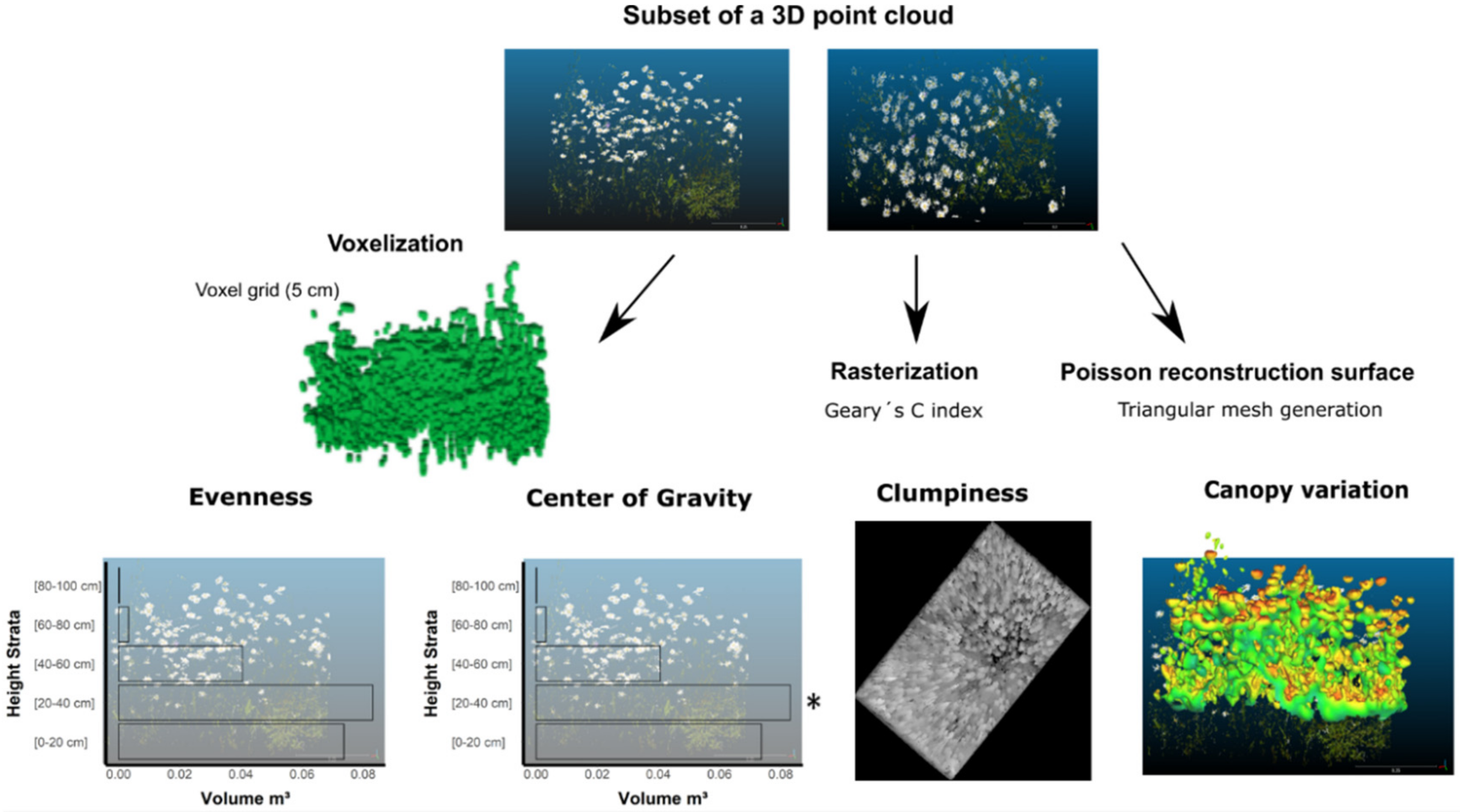
2.2. Terrestrial Laser Scanning: Data Acquisition and Processing

To conduct a non-destructive measurement of the canopy structure at high temporal resolution, we used a terrestrial laser scanner (TLS) Faro Focus 3D X330 [44]. We scanned the 92 plots biweekly from April to September 2014, resulting in 11 time-steps. The TLS was mounted upside-down on a tripod elevated 3.35 m above soil level. The tripod legs were centered on permanent survey markers to guarantee identical scanning areas over time. For each plot, we extracted an area of 3.75 m² (1.5 m × 2.5 m) below the scanner to reduce the effect of leg shadows within scans. The laser scanner measures the distance between the surface of an object and the scanner. The discrete returns of laser beams registered by the laser scanning produce a point cloud image of the surface of the grassland vegetation. The laser device emits an infrared pulse of 1550 nm with a beam divergence of 0.011° (0.19 mrad) at a range of 0.6 to 130 m. The scanning parameters used for resolution were (i) 44.4 million points (full scan) and (ii) the first level of quality (1×) to maximize the efficiency of the scanning processes [44], yielding 3D point clouds with a scan size of 10,154 × 1138 points horizontally × vertically. The point cloud of all scan plots was converted into XYZ coordinates using the proprietary software “Scene” (version 5.2.0, [45]).

We adopted two filtering processes on the point cloud data to reduce errors and promote higher accuracy. First, we applied a statistical outlier removal, which computes the average distance of every sixth point to its neighbors and rejects points that are farther than the average distance (N = 6, ∑ = 1.5). Second, a noise filter removed the points far away from the fitted plane in a plane of 2 mm circumference. The software ‘CloudCompare 2.8.1’ performed both filtering processes using the function SOR [46]. LAS format files were derived from the XYZ coordinates of the point clouds. To obtain height above ground level, we normalized the Z coordinates of the community canopy returns and applied a digital terrain model based on a triangular irregular network (TIN) approach. It is important to note that although Faro Scanner produces discrete-return laser beams that can reduce the information below the canopy, we still believe that, due to the density of points obtained in all plots, it provides a good proxy for the height distribution of structures.

2.2.1. Canopy Structural Components

To characterize the canopy volume of the grassland community, we calculated volume based on the voxelization technique (Figure 1). A ‘voxel grid’ is a digital description of a volumetric object that subdivides the point clouds into a regular grid in three-dimensional space with a defined size [7]. We only used voxels that contained at least one 3D point. To determine the voxel grid size, we checked the density of points per m². To compute the density of points, the number of neighboring points (inside a sphere of radius R = 0.05 m) was counted for each point. As a result, we obtained the volume density classes per cubic meter distribution, which presented a normal distribution as calculated via the Gauss distribution fitting function in the CloudCompare software [46]. Hence, for each scanned plot, a voxel grid with a resolution of 5 cm was created, and the volume was then calculated as the product of the cell area and the attributed height. Further, we split scanned plots based on the voxel grids into five different strata of height (0.3–20 cm, 20–40 cm, 40–60 cm, 60–80 cm, and 80–100 cm). We calculated the sum of all voxels separately for each of the five strata. As a result, we obtained volumetric data based on 3D point clouds for five different strata along the vegetation height.

The vertical metrics of canopy structure components—the evenness and center of gravity—are based on voxel grid estimations of the 3D point clouds for each plot (Figure 1). To measure the evenness of canopy volume along with vegetation height, we calculated:

$$Evenness={\displaystyle \sum }_{i=1}^n(Volum{e}_i/{\displaystyle \sum }_{i=1}^n{(Volum{e}_i)}^2)/5$$

Evenness is the sum of volume proportions of each of the five strata per total volume of the plot divided by 5, where i is each stratum of height and n is the number of plots. The evenness describes the homogeneity of the point cloud density in their vertical distribution. The center of gravity, in turn, used the volume of voxel grids per height strata to identify the location—height stratum (definition see above)—with the highest density of points (adapted from Barry et al., 2020; Spehn et al., 2000). Then, we calculated as follows:

$$Centerofgravity=(Volum{e}_{i=1}^n/{\displaystyle \sum }_{i=1}^n(Volum{e}_i){)}^2$$

Based on calculating the sum of volume proportions along strata of height, we identify the stratum with the highest volume allocated. The center of gravity ranges from 1 to 5, where 1 is the bottom layer (0–20 cm), and 5 is the top canopy (80–100 cm) (Figure 1).

To assess the spatial heterogeneity of the plant community for each plot, we also calculated two horizontal metrics of canopy structural components describing the canopy roughness and clumpiness based on the rasterization of 3D point clouds. We used the surface reconstruction method, which fits a mesh on each plot’s 3D point cloud density (the filtered point clouds and not voxel grids) [47]. We applied the Poisson Surface Reconstruction method, which fits a mesh on all oriented points (perpendicular vectors to the tangential plane to the surface at that point) [48]. After producing the surface mesh for all plots, a surface area of the mesh in square meters was calculated and divided by the area of the plot (3.75 m²) (Figure 1). For clumpiness, we evaluated the size and distribution of clusters in the spatial arrangement of the point cloud into two dimensions based on the rasterized 3D point clouds. For this, we computed Geary’s C index, an identifier of cluster points with similar attributes, assessed by the pixel spatial autocorrelation [49]. The Geary’s C index lies between 0 and some unspecified values greater than 1. Hence, values lower than 1 display an increase in positive spatial autocorrelation (more similar clusters—less clumpiness), while values close and higher than 1 demonstrate increasing negative spatial autocorrelation (more dissimilar clusters—high clumpiness). We used the function Geary from the R package “raster” (Figure 1).

2.3. Data Analyses

Intra-Annual Diversity Effects on Plant Communities Canopy Structure

To investigate the temporal changes in diversity effects on the volume and the canopy structure of grassland communities, we fitted separate mixed-effects models for volume and each metric of canopy structural components using the lme function in the nlme package of the statistical software R (version 3.6.3). We examined the relationship between diversity (experiment design species richness as predictors) and volume and canopy structural component measures (response variables) using the TLS measurements obtained on 11 dates throughout the growing season. We checked for each model if the residuals were temporally auto-correlated (via the ACF function) within the 11 dates [50]. Therefore, the mixed-effects models were fitted with a correlation structure function. First, we assessed the standardized residuals using an empirical autocorrelation plot and compared the performance of models for different auto-correlation structure functions such as AR1 and ARMA (1,0) and ARMA (2,0) with distinct error structures based on AIC values [50]. In the final mixed-effect model, we used the autoregressive correlation structure, which displayed the lowest AIC value (for volume, we used the R function corAR1 (0.5); for the four canopy metrics we used corARMA (2,0); package nlme, version 3.1-128) for the times of measurement [50,51]. The mixed-effects models treated block and plot as random factors in which plots are nested in blocks because we have repeated measurements (11 times) in each plot. Moreover, this parameterization allows responses to vary randomly between blocks and plots throughout the growing season. For all mixed effect models, we chose a parameterization without intercept so that the individual coefficients at each sampling time vary around zero and indicate the occurrence of significant positive or negative effects (instead of expressing the difference to some arbitrary reference sampling time). We fitted all final models with the REML approach of parameter estimation. We assessed the homogeneity of residuals with residuals vs. fitted values plots and Q-Q plots for data normality using “Pearson” correlation [52]. We used the anova function for mixed-effects models using the F-statistic (likelihood ratio test).

3. Results

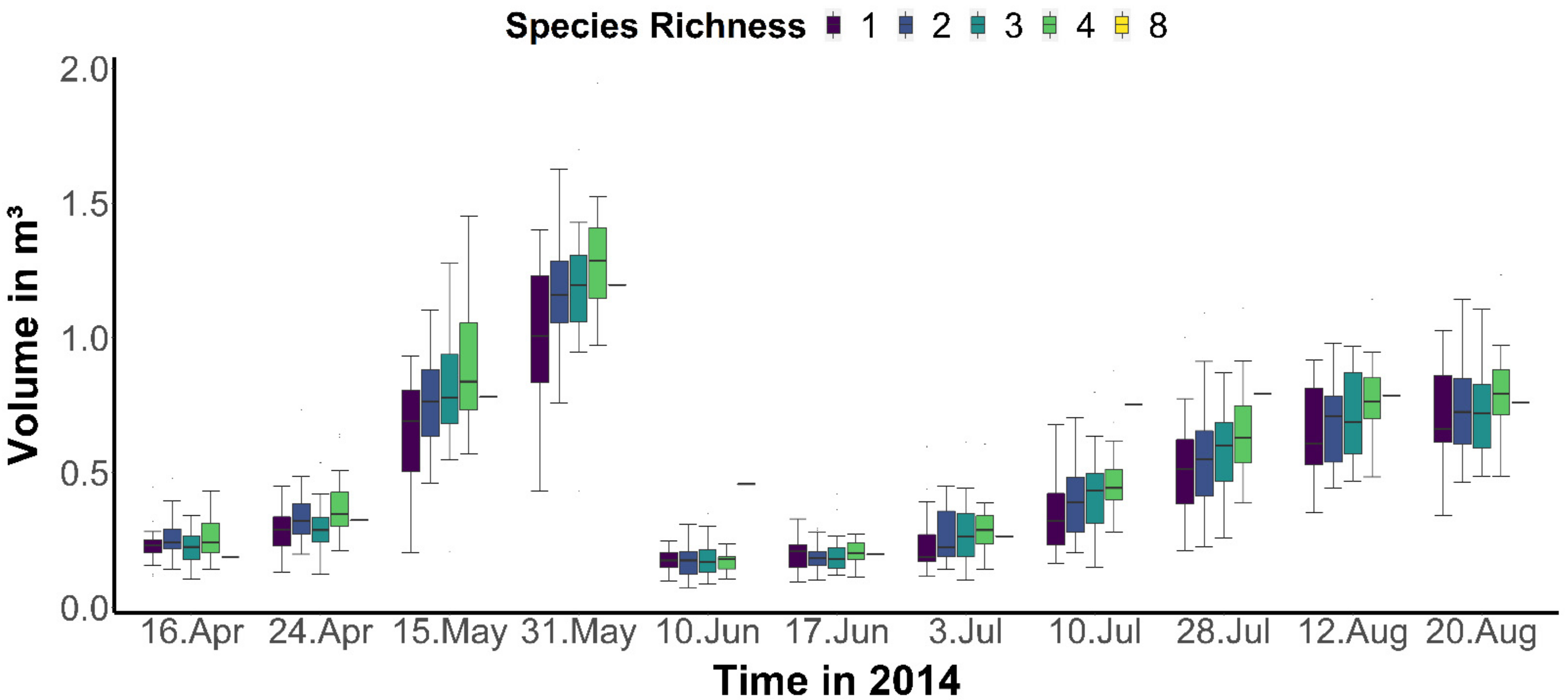
3.1. Plant Diversity Effects on Volume Distribution across the Season

The volume calculated from the voxel grid approach varied strongly across gradients of species richness, the height strata (Figure S1), and throughout the growing season (Figure 2). The TLS point clouds of plant communities showed a high density of points in the lowest layer of the height strata irrespective of the sampling time (Figure S1). This suggests that the TLS sensors provided a good vertical representation of all canopy elements even during biomass peak. Our data show that most of the volume was concentrated between 0.3 to 20 cm (Strata of height 1) (Figure S1).

In a second step, we found that the effect of plant diversity on the total volume per plot changed significantly over time (significant interaction between species richness and time in

Table 1. Type II analysis of variance table with Kenward–Roger’s method showing the results with the fixed-effects part of the mixed-effects models considering the effects of plant species richness (‘SR’) on the total volume over the growing season (“Time”). Restricted maximum likelihood estimated the variance components of the mixed effect models. Values in the columns are numerator degrees of freedom (Df), chi-square test (Chisq), and p-values (Pr (>Chisq)). Significant relationships at level 0.05 are in bold.

	Df	Chisq	Pr (>Chisq)
Time	11	10,122.029	2.2 × 10−16
Time × SR	11	69.421	1.574 × 10−7

). The volume increased with plant diversity, but this relationship was not consistently strong over the growing season (Figure 2 and Figure 3A). We found a significantly positive effect of plant diversity on accumulative volume during the peak of biomass in May (15 and 31 May; p values < 0.001 for both dates, Figure 3A). In addition, after the mowing and during the summer, species richness significantly promoted total volume before the peak of biomass in August (10 and 28 July, 12 August; p values of 0.006, 0.004, and 0.006 respectively; Figure 3A). Notably, there was no significant effect of species richness on total volume at the biomass peak on 20 August (p-value of 0.135).

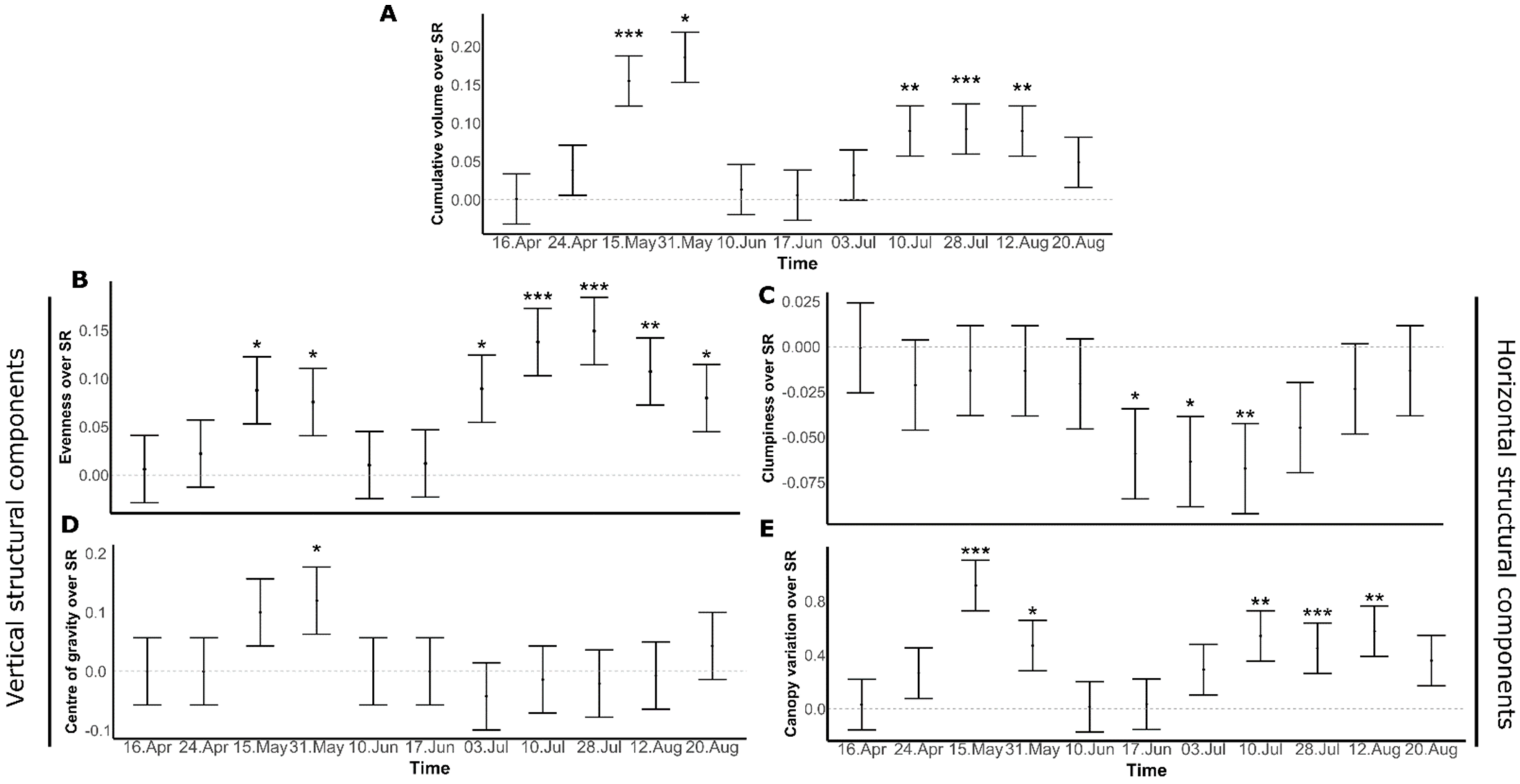
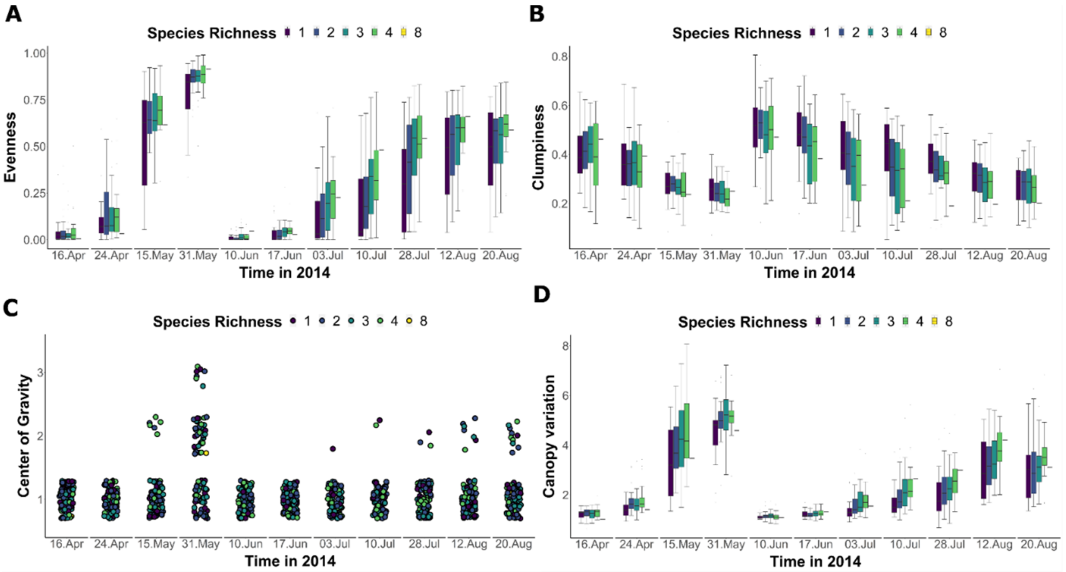
3.2. Seasonal Diversity Effects on Canopy Structural Components

Further, we extracted the slopes for individual dates from mixed effect models to test how diversity affects community canopy structural components over time. Our results show significant differences in the effect of plant diversity on canopy structural component metrics throughout the growing season (Figure 3 and Figure 4). In spring, richer communities presented a more even volume distribution during periods close to the peak of biomass (15 and 31 May, p = 0.01 and p = 0.03, respectively; Figure 3B). In the summer, plant diversity displayed even stronger effects on evenness of volume distribution along the height profile (on 10 July with a p-value of 0.0001 and 28 July, a p-value < 0.0001) than at the biomass peak on 20 August (p-value of 0.02). The center of gravity exhibited the highest volume in the lowest height layer over time (Figure 4C), except for the dates of highest biomass in May and August (Figure 4C). Moreover, the models testing the effects of diversity on the center of gravity showed a significant effect of time, that was, however, independent of species richness (

Table 2. Type II analysis of variance table with Kenward–Roger’s method showing the results with the fixed-effects part of the mixed-effects models considering the effects of diversity (“SR”) on each community canopy structure metrics over the growing season (“time”). Restricted maximum likelihood estimated the variance components of the mixed effect models. Values in the columns are numerator degrees of freedom (Df), chi-square test (Chisq), and p-values (Pr (>Chisq)). Significant relationships are in bold and follow the codes for significant relationships: 0 ‘***’ 0.001 ‘**’ 0.01 ‘*’ 0.05 ‘.’.

Evenness				Clumpiness
	Df	Chisq	Pr (>Chisq)		Df	Chisq	Pr (>Chisq)
time	11	9022.90	<2.2 × 10−16 ***	time	11	2419.695	2 × 10−16 ***
SR × time	11	39.53	4.301 × 10−5 ***	SR × time	11	14.373	0.213
Center of Gravity				Canopy variation
	Df	Chisq	Pr (>Chisq)		Df	Chisq	Pr (>Chisq)
time	11	6038.5361	<2 ×10−16 ***	time	11	4740.987	<2.2 × 10−16 ***
SR × time	11	8.3985	0.6772	SR × time	11	47.521	1.738 × 10−6 ***

). Despite this fact, species richness emerged as a significant predictor for the center of gravity during peak biomass in spring (31 May 31; p = 0.03; Figure 3D).

For the metrics describing the horizontal canopy components, the model testing the effects of diversity on clumpiness showed an overall significant effect with time (Table 2). Even though the analysis of variance of the main effects showed an overall not significant interaction between time and species richness, we found that, by considering only the variation of the slopes, diversity had a negative effect on the clumpiness of vegetation patches during the recovery period after the mowing. The strengths of the negative relationship between clumpiness and species richness, only considering the variation of estimates, increased from 17 June to 10 July (p values varied between 0.01 and 0.007, respectively) but did not remain significant in the consecutive dates when the plant community again filled the available canopy space (Figure 3C). Lastly, canopy variation increased with species richness and time (Figure 4E), but with higher variability in dates just before the biomass peak on 15 May and 12 August (Figure 3E). The canopy variation increased with diversity and particularly at the dates before the peak of biomass (in spring 15 May; p = 0.0001, and in autumn for the days on 10 and 28 July and 12 August; p values of 0.003, 0.01, 0.002, respectively) species richness emerged as a highly significant predictor (Table 2, Figure 3E).

4. Discussion

We expected that the effect of species richness on canopy structural components would differ between vertical and horizontal components and show pronounced but changing effects throughout the growing season related to plant community development over time. For the vertical structural components, we predicted that species richness would positively affect canopy evenness, especially during the peak of biomass due to more intense space-filling along the height profile. In addition, we hypothesized that more diverse and dense swards concentrate leaf biomass at the top of the canopy (higher center of gravity) during phases of intense competition for light. Instead, we found that the strongest influence of plant diversity on canopy evenness occurred at dates well before the peak of biomass and strongly increased after the mowing. This finding demonstrates that in species-rich plant communities, vertical space-filling starts well before the phase of peak biomass in spring and autumn and may lead to an extended period of near-complete absorption of light due to a better three-dimensional canopy arrangement [13]. In line with our expectation, we found that more diverse communities had a higher center of gravity at the biomass peak, but this was only observed in spring. This result indicates that the height of biomass concentration (calculated on a volume basis) during the peak of biomass may result from a higher probability of encountering taller species in diverse communities and stronger etiolation responses and shifts in biomass allocation towards the top canopy due to intense competition for light. We further expected that species richness would influence horizontal clumpiness mainly at the time of lower interspecific interactions (start of the season and after mowing). We found that more diverse communities are clumpier only after mowing, potentially revealing species-specific differences in regrowth. Lastly, as expected, when the differences in phenology status and height were maximal (before the biomass peak), canopy surface variation was most strongly affected by species richness. In summary, our findings revealed that the effect of plant diversity on different components of canopy structure changed throughout the growing season and is not necessarily strongest at the biomass peak. Thus, we presume that diversity effects on ecosystem functions related to canopy structure, such as carbon fluxes, water use efficiency, light availability, and consumer communities within the canopy, may be equally variable over time.

4.1. Diversity Effects on Vertical Metrics of Canopy Structural Components

Vertical metrics of canopy structural components are known to mediate the effects of plant diversity on ecosystem functions, such as carbon gain, gradients in leaf nitrogen concentration relevant for photosynthesis, water use efficiency, and surface temperature [11,34,53,54,55]. These findings result from studies in which canopy structures such as height and density are measured at the peak of biomass of dynamic plant communities such as grasslands. Here, we report that positive plant diversity effects on vertical structural components such as canopy evenness start earlier in the season and are even more important during the recovery period of the vegetation after disturbances such as mowing. These findings suggest that corresponding effects on ecosystem functions mediated by, e.g., a more even vertical leaf distribution, might also vary in response to different gradients of diversity in distinct periods of the growing season. Our results show that canopies of plant mixtures reach high levels of vertical evenness quickly before the peak of biomass in spring and after mowing in summer, thus extending the total time during which canopies are more homogeneously filled with biomass. The circumstance that diverse communities can fill the vertical dimension of the growing space more evenly has been reported earlier, although only from snapshot measurements. It has been argued that the high level of variation in leaf sizes, orientation, and physiology, which is needed to fill the vertical profile evenly, requires interspecific variation rather than the intraspecific variation realized in monocultures [19]. Indirect evidence for the temporal aspect of an extended period of even space-filling comes from a study conducted by [14], who showed that in diverse mixtures, shorter species started to grow earlier, storing resources earlier in the season to compensate for the light competition from taller species later on at the peak of biomass. Moreover, there is a trade-off between height and leaf area, meaning that plants that invest earlier in leaf area at the beginning of the growing season, such as young rosette plants, may not grow taller and fill the canopy space from bottom to top close to the peak of biomass [56]. This strategy leaves space for taller species that do not grow many leaves in the lower strata of the canopy but are specialized at exploiting the light more at the top of the canopy (often tall herb species or tall-statured grasses) towards the peak of biomass. This scenario might explain our results in the sense that the canopy is filling over time with shorter species with more leaves close to the ground and taller species with leaves closer to the upper layer of the canopy, resulting in a canopy with higher evenness before the peak of biomass already in May. This pattern also reflects interspecific differences in biomass allocation across the growing season and allows the “division of labor” in mixtures which may promote ecosystem functioning by stacking more biomass into a given canopy space and improving light-harvesting [55]. At the end of the growing season, we observed richer communities having a more even vertical canopy distribution. However, another process might play a role within plant communities. The phenological stages of plant species may impact canopy structure in more diverse communities. Between 3 July and 12 August is a period of biomass increase after the recovery from the first mowing. Still, it is also a period in which plants face nutrient deficiency and less water than in spring, leading to early senescence. For instance, most grass species reduced their leaf greenness in more diverse communities [11], reflecting leaf senescence in the upper canopy layers. This gives space for tall and short herbs, with late flowering phenology taking over the job of forming a dense and low canopy dominated by small herbs. Ref. [57] showed that at the end of the growing season, plant communities with more inter-specific interactions (as expected in more diverse communities) increased leaf area index exhibiting a denser canopy, despite senescing leaves dropping from the upper layer of the canopy. In our case, despite lower overall heights and a potential earlier start of leaf senescence of some species in August, mixtures still provided a more even vertical canopy distribution likely due to higher interspecific interactions of late flowering species.

In our study, a positive influence of plant diversity on the center of gravity commenced in mid-May and became significant on 31 May when the center of gravity was raised to 60 cm (stratum 3) in more diverse communities. As biomass reaches its maximum and canopy height increases, it is expected that species-rich communities potentially trigger a strong asymmetric competition for light. Moreover, as in our study, grass-dominated communities are known to develop and flower earlier in the season [40]. It is, therefore, reasonable to assume that the height increase, reflected by a higher center of gravity in richer communities, might be due to grass species with long leaves such as Dactylis glomerata L. and Helictotrichon pubescens (Huds.) Pilg. After the mowing, there was no evidence of plant diversity effects on the center of gravity. Likely, as the swards from 3 June to 20 August started displaying a more evenly distributed volume (Figure 3A) within the canopy, a prominent layer of more biomass accumulation was not detected in more diverse communities. This scenario reveals an opposing mechanism between evenness and the center of gravity at this time of the growing season. Although it is known that more diverse communities potentially increase the center of gravity due to high competition for light at high densities [13], at the recovery period after the mowing, biomass production of plant communities is lower compared to spring and is mostly allocated at the lower layer of the canopy which increases canopy evenness in species-rich communities. Roscher et al. (2011) observed that the highest photosynthetic activity was detected mainly at lower canopy layers from the middle of August onwards. This result was attributed to small-statured species (such as Prunella vulgaris L. present in our experiment) that have a greater capacity to grow under unfavorable conditions, such as low light availability when the canopy becomes denser at the peak of biomass. These findings could support our explanation for the lack of diversity effects on the center of gravity and the concomitant increase in canopy evenness since functional strategies of plant species might contribute to filling the canopy space from bottom to top, preventing a higher biomass allocation at the top layers of the canopy at the end of the growing season.

4.2. Diversity Effects on Horizontal Components of Canopy Structure

The way that plant species are spatially aggregated or forming areas of clumping within the communities are also potential drivers of biodiversity–ecosystem functioning relationships [58,59]. This is because interspecific interactions between close neighbors can cause different diversity effects (i.e., resource use complementarity, the selective dominance of more productive species, abiotic facilitation [2,58,60]. Here we predicted that plant communities’ degree of aggregation or clumpiness would change over time and would be lower in species-rich communities due to higher interspecific interactions, forcing species to arrange to finer-grained patterns spatially. Indeed, we found that species-rich communities were less clumpy than species-poor communities and this was particularly pronounced during the second part of the growing season (four weeks after mowing).

These findings support the assumptions that diversity has a negative effect on clumpiness as already tested in conceptual mathematical models [61,62] and in experiments considering only the peak of biomass [20,59]. However, for the first time, we showed that this negative effect of diversity on clumpiness is not consistent over the growing season and is much more pronounced later in the season than earlier. One potential reason for the strong seasonality in diversity effects on clumpiness could be that plant species show phenological asymmetry which might lead to prolonged periods of low plant–plant interaction. In addition to the phenological asymmetry, there is a higher likelihood of having stronger competitors in more diverse communities [63,64,65]. This is both true for Geranium pratensis L., which is a dominant and late flowering species. The species is known for forming dense patches of fast sprouting leaves in the beginning of the growing season but even more so during the recovery period after mowing due to extensive belowground storage organs. This may contribute to an increase in community clumpiness especially during re-sprouting. However, as plants grow taller between June and July, G. pratensis leaves form a dense, homogeneous canopy which might decrease community clumpiness by covering neighboring plants towards the peak of summer biomass [66]. Hence, our study endorses that the degree of clumpiness (spatial aggregation) may serve as a potential parameter to understand the temporal variation of intra- and interspecific competition within plant communities and how it influences biodiversity–ecosystem functioning relationships.

Our findings support our hypothesis that species richness increases canopy variation when height differences are highest between species, which would occur midway between the onset of the growing season and the biomass peak. Our results likely reflect that species-rich communities contain species with larger architectural differences, such as a broader range of statures and inflorescence types and distinct flowering phenology. In contrast, species-poor communities consist of a more comparable height, structure, and more similar flowering patterns [67]. The differences in plant species’ phenological characteristics and resource use may promote temporal growth variation mainly expressed by plant height variation, as found in [67]. In the midway of the development towards the peak of biomass, species-rich communities containing early flowering species might already grow taller than species with late phenology that did not have enough time to increase in height. This scenario is observed in both growing periods (before and after mowing) but is more pronounced in summer in our data. In our experiment, the grasses Anthoxanthum odoratum L., Dactylis glomerata, and Helictotrichon pubescens (Huds.) Pilg. mainly flower in May together with a small-statured forb (Plantago lanceolata L.) and a tall herb (Leucanthemum vulgare Lam.). These species grow tall early in the season while late-flowering species, such as the tall herb Geranium pratensis, the small herb Prunella vulgaris, and the grasses Festuca rubra L. and Holcus lanatus L. only catch up and reduce overall canopy variation at peak biomass. These differences in height may have contributed to the high correlation between species richness and canopy variation on 15 and 31 May. After the first mowing, species richness increased canopy variation even more strongly from 10 June to 12 August. Multiple, not mutually exclusive, factors might explain the strong positive effects of diversity on canopy variation in summer. First, the late-flowering species recover faster and have a substantial effect on canopy variation midway during summer, the same as early-flowering species in spring. Second, the cumulative volume of plant communities along the species richness gradient also reveals a strong positive signal of diversity effects on the total volume between 10 July to 12 August. During this period, there was a clear increase in volume from 0.3 to 20 cm and from 20 to 40 cm of the canopy layers. However, after 12 August, this signal on total volume disappeared, as did the effect on canopy variation. Therefore, late phenology species, high photosynthetic activity, and total volume associated with diverse communities midway during recovery after mowing and the second biomass peak might support our results.

Our study shows that plant diversity effects on different canopy structural components extend our understanding of biodiversity–ecosystem functioning relationships, as the effects vary largely across the growing season and are not necessarily strongest at the biomass peak. We also observed that the duration of positive structural features, such as evenness, is positively related to diversity. Hence, the effects of diversity on ecosystem functions depending on structural components, such as biomass production, decomposition, and herbivory, may change throughout the season due to various mechanisms, such as niche differences, increased complementarity, and temporal and spatial variation in biological activity. We show that non-destructive techniques such as terrestrial laser scanning improve our capacity to screen vegetation changes with high temporal and spatial resolution. Future studies should invest in combining different technologies such as hyperspectral signal and structural data from TLS to automatically identify species and estimate their distribution and relative abundances. Further, simultaneously examining the temporal and spatial variation of belowground and aboveground organisms and their activities [68] would expand our understanding of long-term ecosystem functioning, since their inter-relation may determine the total ecosystem production and stability and multifunctionality.

References

1. Barry, K.E.; Weigelt, A.; van Ruijven, J.; de Kroon, H.; Ebeling, A.; Eisenhauer, N.; Gessler, A.; Ravenek, J.M.; Scherer-Lorenzen, M.; Oram, N.J.; et al. Above- and Belowground Overyielding Are Related at the Community and Species Level in a Grassland Biodiversity Experiment. In Advances in Ecological Research; Elsevier: Amsterdam, The Netherlands, 2019; Volume 61, pp. 55–89. ISBN 978-0-08-102912-1. [Google Scholar]
2. Cardinale, B.J.; Duffy, J.E.; Gonzalez, A.; Hooper, D.U.; Perrings, C.; Venail, P.; Narwani, A.; Mace, G.M.; Tilman, D.; Wardle, D.A. Biodiversity Loss and Its Impact on Humanity. Nature 2012, 486, 59–67. [Google Scholar] [CrossRef] [PubMed]
3. Lange, M.; Roth, V.; Eisenhauer, N.; Roscher, C.; Dittmar, T.; Fischer-Bedtke, C.; González Macé, O.; Hildebrandt, A.; Milcu, A.; Mommer, L.; et al. Plant Diversity Enhances Production and Downward Transport of Biodegradable Dissolved Organic Matter. J. Ecol. 2021, 109, 1284–1297. [Google Scholar] [CrossRef]
4. Reich, P.B.; Tilman, D.; Isbell, F.; Mueller, K.; Hobbie, S.E.; Flynn, D.F.; Eisenhauer, N. Impacts of Biodiversity Loss Escalate through Time as Redundancy Fades. Science 2012, 336, 589–592. [Google Scholar] [CrossRef] [PubMed] [Green Version]
5. Xu, S.; Eisenhauer, N.; Ferlian, O.; Zhang, J.; Zhou, G.; Lu, X.; Liu, C.; Zhang, D. Species Richness Promotes Ecosystem Carbon Storage: Evidence from Biodiversity-Ecosystem Functioning Experiments. Proc. R. Soc. B. 2020, 287, 20202063. [Google Scholar] [CrossRef]
6. Cooper, S.; Roy, D.; Schaaf, C.; Paynter, I. Examination of the Potential of Terrestrial Laser Scanning and Structure-from-Motion Photogrammetry for Rapid Nondestructive Field Measurement of Grass Biomass. Remote Sens. 2017, 9, 531. [Google Scholar] [CrossRef] [Green Version]
7. Schulze-Brüninghoff, D.; Hensgen, F.; Wachendorf, M.; Astor, T. Methods for LiDAR-Based Estimation of Extensive Grassland Biomass. Comput. Electron. Agric. 2019, 156, 693–699. [Google Scholar] [CrossRef]
8. Wallace, L.; Hillman, S.; Reinke, K.; Hally, B. Non-destructive Estimation of Above-ground Surface and Near-surface Biomass Using 3D Terrestrial Remote Sensing Techniques. Methods Ecol. Evol. 2017, 8, 1607–1616. [Google Scholar] [CrossRef] [Green Version]
9. Guimarães-Steinicke, C.; Weigelt, A.; Ebeling, A.; Eisenhauer, N.; Duque-Lazo, J.; Reu, B.; Roscher, C.; Schumacher, J.; Wagg, C.; Wirth, C. Terrestrial Laser Scanning Reveals Temporal Changes in Biodiversity Mechanisms Driving Grassland Productivity. In Advances in Ecological Research; Elsevier: Amsterdam, The Netherlands, 2019; Volume 61, pp. 133–161. ISBN 978-0-08-102912-1. [Google Scholar]
10. Schuldt, A.; Ebeling, A.; Kunz, M.; Staab, M.; Guimarães-Steinicke, C.; Bachmann, D.; Buchmann, N.; Durka, W.; Fichtner, A.; Fornoff, F.; et al. Multiple Plant Diversity Components Drive Consumer Communities across Ecosystems. Nat. Commun. 2019, 10, 1460. [Google Scholar] [CrossRef] [Green Version]
11. Bachmann, D.; Roscher, C.; Buchmann, N. How Do Leaf Trait Values Change Spatially and Temporally with Light Availability in a Grassland Diversity Experiment? Oikos 2018, 127, 935–948. [Google Scholar] [CrossRef]
12. Wang, R.; Gamon, J.; Montgomery, R.; Townsend, P.; Zygielbaum, A.; Bitan, K.; Tilman, D.; Cavender-Bares, J. Seasonal Variation in the NDVI–Species Richness Relationship in a Prairie Grassland Experiment (Cedar Creek). Remote Sens. 2016, 8, 128. [Google Scholar] [CrossRef] [Green Version]
13. Spehn, E.M.; Joshi, J.; Schmid, B.; Diemer, M.; Korner, C. Above-Ground Resource Use Increases with Plant Species Richness in Experimental Grassland Ecosystems. Funct. Ecol. 2000, 14, 326–337. [Google Scholar]
14. Anten, N.P.R.; Hirose, T. Interspecific Differences in Above-Ground Growth Patterns Result in Spatial and Temporal Partitioning of Light among Species in a Tall-Grass Meadow. J. Ecol. 1999, 87, 583–597. [Google Scholar] [CrossRef]
15. Hirose, T.; Werger, M.J.A. Canopy Structure and Photon Flux Partitioning Among Species in a Herbaceous Plant Community. Ecology 1995, 76, 466–474. [Google Scholar] [CrossRef]
16. Wacker, L.; Baudois, O.; Eichenberger-Glinz, S.; Schmid, B. Environmental Heterogeneity Increases Complementarity in Experimental Grassland Communities. Basic Appl. Ecol. 2008, 9, 467–474. [Google Scholar] [CrossRef] [Green Version]
17. Williams, L.J.; Paquette, A.; Cavender-Bares, J.; Messier, C.; Reich, P.B. Spatial Complementarity in Tree Crowns Explains Overyielding in Species Mixtures. Nat. Ecol. Evol. 2017, 1, 0063. [Google Scholar] [CrossRef]
18. Barry, K.E.; Ruijven, J.; Mommer, L.; Bai, Y.; Beierkuhnlein, C.; Buchmann, N.; Kroon, H.; Ebeling, A.; Eisenhauer, N.; Guimarães-Steinicke, C.; et al. Limited Evidence for Spatial Resource Partitioning across Temperate Grassland Biodiversity Experiments. Ecology 2020, 101, e02905. [Google Scholar] [CrossRef] [Green Version]
19. Dimitrakopoulos, P.G.; Schmid, B. Biodiversity Effects Increase Linearly with Biotope Space: Diversity Effects Increase with Biotope Space. Ecol. Lett. 2004, 7, 574–583. [Google Scholar] [CrossRef]
20. Lorentzen, S.; Roscher, C.; Schumacher, J.; Schulze, E.-D.; Schmid, B. Species Richness and Identity Affect the Use of Aboveground Space in Experimental Grasslands. Perspect. Plant Ecol. Evol. Syst. 2008, 10, 73–87. [Google Scholar] [CrossRef] [Green Version]
21. Ratcliffe, S.; Liebergesell, M.; Ruiz-Benito, P.; Madrigal González, J.; Muñoz Castañeda, J.M.; Kändler, G.; Lehtonen, A.; Dahlgren, J.; Kattge, J.; Peñuelas, J.; et al. Modes of Functional Biodiversity Control on Tree Productivity across the European Continent: Functional Biodiversity Control on Tree Growth. Glob. Ecol. Biogeogr. 2016, 25, 251–262. [Google Scholar] [CrossRef] [Green Version]
22. Walter, J.A.; Stovall, A.E.L.; Atkins, J.W. Vegetation Structural Complexity and Biodiversity in the Great Smoky Mountains. Ecosphere 2021, 12, e03390. [Google Scholar] [CrossRef]
23. Marquard, E.; Weigelt, A.; Roscher, C.; Gubsch, M.; Lipowsky, A.; Schmid, B. Positive Biodiversity-Productivity Relationship Due to Increased Plant Density. J. Ecol. 2009, 97, 696–704. [Google Scholar] [CrossRef] [Green Version]
24. Hertzog, L.R.; Meyer, S.T.; Weisser, W.W.; Ebeling, A. Experimental Manipulation of Grassland Plant Diversity Induces Complex Shifts in Aboveground Arthropod Diversity. PLoS ONE 2016, 11, e0148768. [Google Scholar] [CrossRef]
25. Eisenhauer, N.; Reich, P.B.; Scheu, S. Increasing Plant Diversity Effects on Productivity with Time Due to Delayed Soil Biota Effects on Plants. Basic Appl. Ecol. 2012, 13, 571–578. [Google Scholar] [CrossRef]
26. Hobbs, R.J.; Yates, S.; Mooney, H.A. Long-term data reveal complex dynamics in grassland in relation to climate and disturbance. Ecol. Monogr. 2007, 77, 545–568. [Google Scholar] [CrossRef]
27. Jones, S.K.; Ripplinger, J.; Collins, S.L. Species Reordering, Not Changes in Richness, Drives Long-term Dynamics in Grassland Communities. Ecol. Lett. 2017, 20, 1556–1565. [Google Scholar] [CrossRef]
28. Moorsel, S.J.; Hahl, T.; Petchey, O.L.; Ebeling, A.; Eisenhauer, N.; Schmid, B.; Wagg, C. Co-occurrence History Increases Ecosystem Stability and Resilience in Experimental Plant Communities. Ecology 2021, 102. [Google Scholar] [CrossRef]
29. Weisser, W.W.; Roscher, C.; Meyer, S.T.; Ebeling, A.; Luo, G.; Allan, E.; Beßler, H.; Barnard, R.L.; Buchmann, N.; Buscot, F.; et al. Biodiversity Effects on Ecosystem Functioning in a 15-Year Grassland Experiment: Patterns, Mechanisms, and Open Questions. Basic Appl. Ecol. 2017, 23, 1–73. [Google Scholar] [CrossRef]
30. Zhang, Z.; Cao, L.; She, G. Estimating Forest Structural Parameters Using Canopy Metrics Derived from Airborne LiDAR Data in Subtropical Forests. Remote Sens. 2017, 9, 940. [Google Scholar] [CrossRef] [Green Version]
31. Liira, J.; Zobel, K.; Mägi, R.; Molenberghs, G. Vertical Structure of Herbaceous Canopies: The Importance of Plant Growth-Form and Species-Specific Traits. Plant Ecol. 2002, 163, 123–134. [Google Scholar] [CrossRef]
32. Spehn, E.M.; Hector, A.; Joshi, J.; Scherer-Lorenzen, M.; Schmid, B.; Bazeley-White, E.; Beierkuhnlein, C.; Caldeira, M.C.; Diemer, M.; Dimitrakopoulos, P.G.; et al. Ecosystem Effects of Biodiversity Manipulations in European Grasslands. Ecol. Monogr. 2005, 75, 37–63. [Google Scholar]
33. Leger, E.A.; Espeland, E.K. The Shifting Balance of Facilitation and Competition Affects the Outcome of Intra- and Interspecific Interactions over the Life History of California Grassland Annuals. Plant Ecol. 2010, 208, 333–345. [Google Scholar] [CrossRef]
34. Guimarães-Steinicke, C.; Weigelt, A.; Proulx, R.; Lanners, T.; Eisenhauer, N.; Duque-Lazo, J.; Reu, B.; Roscher, C.; Wagg, C.; Buchmann, N.; et al. Biodiversity Facets Affect Community Surface Temperature via 3D Canopy Structure in Grassland Communities. J. Ecol. 2021, 109, 1969–1985. [Google Scholar] [CrossRef]
35. Atkins, J.W.; Bohrer, G.; Fahey, R.T.; Hardiman, B.S.; Morin, T.H.; Stovall, A.E.L.; Zimmerman, N.; Gough, C.M. Quantifying Vegetation and Canopy Structural Complexity from Terrestrial Li DAR Data Using the forestr r Package. Methods Ecol. Evol. 2018, 9, 2057–2066. [Google Scholar] [CrossRef]
36. Ehbrecht, M.; Schall, P.; Ammer, C.; Seidel, D. Quantifying Stand Structural Complexity and Its Relationship with Forest Management, Tree Species Diversity and Microclimate. Agric. For. Meteorol. 2017, 242, 1–9. [Google Scholar] [CrossRef]
37. Atkins, J.W.; Fahey, R.T.; Hardiman, B.H.; Gough, C.M. Forest Canopy Structural Complexity and Light Absorption Relationships at the Subcontinental Scale. J. Geophys. Res. Biogeosci. 2018, 123, 1387–1405. [Google Scholar] [CrossRef]
38. Stark, S.C.; Enquist, B.J.; Saleska, S.R.; Leitold, V.; Schietti, J.; Longo, M.; Alves, L.F.; Camargo, P.B.; Oliveira, R.C. Linking Canopy Leaf Area and Light Environments with Tree Size Distributions to Explain Amazon Forest Demography. Ecol. Lett. 2015, 18, 636–645. [Google Scholar] [CrossRef]
39. Hardiman, B.S.; Gough, C.M.; Halperin, A.; Hofmeister, K.L.; Nave, L.E.; Bohrer, G.; Curtis, P.S. Maintaining High Rates of Carbon Storage in Old Forests: A Mechanism Linking Canopy Structure to Forest Function. For. Ecol. Manag. 2013, 298, 111–119. [Google Scholar] [CrossRef]
40. Ebeling, A.; Pompe, S.; Baade, J.; Eisenhauer, N.; Hillebrand, H.; Proulx, R.; Roscher, C.; Schmid, B.; Wirth, C.; Weisser, W.W. A Trait-Based Experimental Approach to Understand the Mechanisms Underlying Biodiversity–Ecosystem Functioning Relationships. Basic Appl. Ecol. 2014, 15, 229–240. [Google Scholar] [CrossRef] [Green Version]
41. Roscher, C.; Schumacher, J.; Baade, J.; Wilcke, W.; Gleixner, G.; Weisser, W.W.; Schmid, B.; Schulze, E.-D. The Role of Biodiversity for Element Cycling and Trophic Interactions: An Experimental Approach in a Grassland Community. Basic Appl. Ecol. 2004, 5, 107–121. [Google Scholar] [CrossRef]
42. Bongers, F.J.; Schmid, B.; Bruelheide, H.; Bongers, F.; Li, S.; von Oheimb, G.; Li, Y.; Cheng, A.; Ma, K.; Liu, X. Functional Diversity Effects on Productivity Increase with Age in a Forest Biodiversity Experiment. Nat. Ecol. Evol. 2021, 5, 1594–1603. [Google Scholar] [CrossRef]
43. Zuppinger-Dingley, D.; Schmid, B.; Petermann, J.S.; Yadav, V.; De Deyn, G.B.; Flynn, D.F. Selection for Niche Differentiation in Plant Communities Increases Biodiversity Effects. Nature 2014, 515, 108–111. [Google Scholar] [CrossRef]
44. FARO Technologies Inc. FARO Laser Scaner Focus 3D Instruction Manual; FARO Technologies Inc.: Lake Mary, FL, USA, 2011. [Google Scholar]
45. SCENE User Manual. 2021. Available online: https://knowledge.faro.com/Software/FARO_SCENE/SCENE/User_Manual_for_SCENE (accessed on 16 February 2022).
46. CloudCompare Omnia. 2019. Available online: https://www.cloudcompare.org/release/notes/20200614/ (accessed on 16 February 2022).
47. Attene, M.; Spagnuolo, M. Automatic Surface Reconstruction from Point Sets in Space. Comput. Graph. Forum 2000, 19, 457–465. [Google Scholar] [CrossRef]
48. Kazhdan, M.; Hoppe, H. An Adaptive Multi-Grid Solver for Applications in Computer Graphics. Comput. Graph. Forum 2019, 38, 138–150. [Google Scholar] [CrossRef] [Green Version]
49. Geary, R.C. The Contiguity Ratio and Statistical Mapping. Inc. Stat. 1954, 5, 115. [Google Scholar] [CrossRef]
50. Pinheiro, J.C.; Bates, D.M. Mixed-Effects Models in Sand S-PLUS. In Statistics and Computing; Springer New York: New York, NY, USA, 2000; ISBN 978-1-4419-0317-4. [Google Scholar]
51. Chi, E.M.; Reinsel, G.C. Models for Longitudinal Data with Random Effects and AR(1) Errors. J. Am. Stat. Assoc. 1989, 84, 452–459. [Google Scholar] [CrossRef]
52. Zuur, A.F.; Ieno, E.N.; Walker, N.; Saveliev, A.A.; Smith, G.M. Mixed Effects Models and Extensions in Ecology with R. In Statistics for Biology and Health; Springer: New York, NY, USA, 2009; ISBN 978-0-387-87457-9. [Google Scholar]
53. Milcu, A.; Roscher, C.; Gessler, A.; Bachmann, D.; Gockele, A.; Guderle, M.; Landais, D.; Piel, C.; Escape, C.; Devidal, S.; et al. Functional Diversity of Leaf Nitrogen Concentrations Drives Grassland Carbon Fluxes. Ecol. Lett. 2014, 17, 435–444. [Google Scholar] [CrossRef]
54. Milcu, A.; Gessler, A.; Roscher, C.; Rose, L.; Kayler, Z.; Bachmann, D.; Pirhofer-Walzl, K.; Zavadlav, S.; Galiano, L.; Buchmann, T.; et al. Top Canopy Nitrogen Allocation Linked to Increased Grassland Carbon Uptake in Stands of Varying Species Richness. Sci. Rep. 2017, 7, 8392. [Google Scholar] [CrossRef]
55. Wacker, L.; Baudois, O.; Eichenberger-Glinz, S.; Schmid, B. Effects of Plant Species Richness on Stand Structure and Productivity. J. Plant Ecol. 2009, 2, 95–106. [Google Scholar] [CrossRef]
56. Anten, N.P.R. Optimal Photosynthetic Characteristics of Individual Plants in Vegetation Stands and Implications for Species Coexistence. Ann. Bot. 2004, 95, 495–506. [Google Scholar] [CrossRef] [Green Version]
57. Hikosaka, K.; Anten, N.P.R. An Evolutionary Game of Leaf Dynamics and Its Consequences for Canopy Structure. Funct Ecol 2012, 26, 1024–1032. [Google Scholar] [CrossRef]
58. Fridley, J.D. The Influence of Species Diversity on Ecosystem Productivity: How, Where, and Why? Oikos 2001, 93, 514–526. [Google Scholar] [CrossRef]
59. Peer, L.V.; Nijs, I.; Bogaert, J.; Verelst, I.; Reheul, D. Survival, Gap Formation, and Recovery Dynamics in Grassland Ecosystems Exposed to Heat Extremes: The Role of Species Richness. Ecosystems 2001, 4, 797–806. [Google Scholar] [CrossRef] [Green Version]
60. Barry, K.E.; Mommer, L.; van Ruijven, J.; Wirth, C.; Wright, A.J.; Bai, Y.; Connolly, J.; De Deyn, G.B.; de Kroon, H.; Isbell, F.; et al. The Future of Complementarity: Disentangling Causes from Consequences. Trends Ecol. Evol. 2019, 34, 167–180. [Google Scholar] [CrossRef] [Green Version]
61. De Boeck, H.J.; Nijs, I.; Lemmens, C.M.H.M.; Ceulemans, R. Underlying Effects of Spatial Aggregation (Clumping) in Relationships between Plant Diversity and Resource Uptake. Oikos 2006, 113, 269–278. [Google Scholar] [CrossRef]
62. Tilman, D.; Lehman, C.; Thompson, K. Plant Diversity and Ecosystem Productivity: Theoretical Considerations. Proc. Natl. Acad. Sci. USA 1997, 94, 1857–1861. [Google Scholar] [CrossRef] [Green Version]
63. Aarssen, L.W. High Productivity in Grassland Ecosystems: Effected by Species Diversity or Productive Species? Oikos 1997, 80, 183–184. [Google Scholar] [CrossRef]
64. Fargione, J.; Tilman, D. Plant Species Traits and Capacity for Resource Reduction Predict Yield and Abundance under Competition in Nitrogen-Limited Grassland. Funct. Ecol. 2006, 20, 533–540. [Google Scholar] [CrossRef]
65. Grime, J.P. Benefits of Plant Diversity to Ecosystems: Immediate, Filter and Founder Effects. J. Ecol. 1998, 86, 902–910. [Google Scholar] [CrossRef]
66. Turnbull, L.A.; Coomes, D.A.; Purves, D.W.; Rees, M. How Spatial Structure Alters Population and Community Dynamics in a Natural Plant Community. J. Ecol. 2007, 95, 79–89. [Google Scholar] [CrossRef]
67. Proulx, R.; Roca, I.T.; Cuadra, F.S.; Seiferling, I.; Wirth, C. A Novel Photographic Approach for Monitoring the Structural Heterogeneity and Diversity of Grassland Ecosystems. J. Plant Ecol. 2014, 7, 518–525. [Google Scholar] [CrossRef] [Green Version]
68. Eisenhauer, N.; Herrmann, S.; Hines, J.; Buscot, F.; Siebert, J.; Thakur, M.P. The Dark Side of Animal Phenology. Trends Ecol. Evol. 2018, 33, 898–901. [Google Scholar] [CrossRef] [PubMed]
Figure 1. Visualization of the canopy structural component metrics using a subset of 3D point clouds of a sampling plot in which we calculated volume based on voxel grids with a resolution size of 5 cm. The volume is distributed in 5 height strata varying from (1: 0.3–20 cm, 2: 20–40 cm, 3: 40–60 cm, 4: 60–80 cm, and 5: 80–100 cm) and used to measure evenness and center of gravity indicated by the *. Further, the 3D point clouds were rasterized to calculate Geary’s C index (clumpiness); and using Poisson reconstruction surface of canopy surface, we calculate canopy variation by dividing the canopy surface area by the area of the ground plot. More details described in Methods the section about canopy structural components.
Remotesensing 14 01557 g001
Figure 2. Temporal distribution of total volume per time slice throughout the growing season in 2014. The total volume calculated based on voxelization technique is displayed across the experimental species richness gradient in colored code. Note that the eight-species communities represent two communities in our database, therefore the mean lines have lower variance than other communities and the interquartile ranges in the boxplot are not shown.
Remotesensing 14 01557 g002
Figure 3. Coefficient plot showing the variation of estimates (effect sizes) of species richness (SR), its contrast to zero with 95% confidence intervals. (A) shows the slope each of the cumulative volume and (B) for evenness, (C) for Clumpiness, (D) for center of gravity, and (E) for canopy variation. The slopes are based on mixed-effects models during the growing season in 2014 with codes for significant relationships: 0 ‘***’ 0.001 ‘**’ 0.01 ‘*’ 0.05 ‘.’.
Remotesensing 14 01557 g003
Figure 4. Temporal distribution of four community canopy structural components throughout the growing season: (A) evenness (calculated as the sum of volume proportions of each of the five strata per total volume of the plot divided by 5); (B) clumpiness (calculated via Geary’s (C) index that measures the spatial distribution of clusters in the rasterized 3D point cloud for each plot where values close to zero indicates less clumpiness (similar clusters) while values close to 1 display high clumpiness (dissimilar clusters)); (C) center of gravity (displayed as a categorical measure of the strata of height with the highest volume proportion to the total volume per 5 strata); (D) canopy variation (calculated as the area of fitted surface mesh on the canopy divided by plot area). See details in Section 2.2.1.
Remotesensing 14 01557 g004