Article

Woody Plant Encroachment: Evaluating Methodologies for Semiarid Woody Species Classification from Drone Images

Department of Ecology & Conservation Biology, Texas A&M University, College Station, TX 77598, USA
*
Author to whom correspondence should be addressed.
Submission received: 11 February 2022 / Revised: 21 March 2022 / Accepted: 25 March 2022 / Published: 30 March 2022

Abstract

:
Globally, native semiarid grasslands and savannas have experienced a densification of woody plant species—leading to a multitude of environmental, economic, and cultural changes. These encroached areas are unique in that the diversity of tree species is small, but at the same time the individual species possess diverse phenological responses. The overall goal of this study was to evaluate the ability of very high resolution drone imagery to accurately map species of woody plants encroaching on semiarid grasslands. For a site in the Edwards Plateau ecoregion of central Texas, we used affordable, very high resolution drone imagery to which we applied maximum likelihood (ML), support vector machine (SVM), random forest (RF), and VGG-19 convolutional neural network (CNN) algorithms in combination with pixel-based (with and without post-processing) and object-based (small and large) classification methods. Based on test sample data (n = 1000) the VGG-19 CNN model achieved the highest overall accuracy (96.9%). SVM came in second with an average classification accuracy of 91.2% across all methods, followed by RF (89.7%) and ML (86.8%). Overall, our findings show that RGB drone sensors are indeed capable of providing highly accurate classifications of woody plant species in semiarid landscapes—comparable to and even greater in some regards to those achieved by aerial and drone imagery using hyperspectral sensors in more diverse landscapes.

Graphical Abstract

1. Introduction

Native semiarid grasslands and savannas across the globe are increasingly affected by woody plant encroachment, a phenomenon that leads to fundamental state shifts, whereby herbaceous-dominated landscapes are converted to landscapes more similar to forests and dense shrublands. Increases in woody cover can result in myriad significant changes to a region’s ecology, economy, and culture [1]. The Edwards Plateau ecological region of central Texas (93,000 km2), USA, has been historically maintained as a savanna community by fuel–fire feedbacks driven by the grazing habits of native megafauna. However, over the last 150 years, in response to the combined effects of overgrazing, fire suppression, and climate change, this region of Texas has experienced accelerated encroachment of woody plants [2]. The four main woody species encroaching into native savannas in this region are live oak (Quercus virginiana), blueberry juniper (Juniperus Ashei), redberry juniper (Juniperus Pinchotii), and honey mesquite (Prosopis glandulosa). The effects of this expansion on the region’s hydrological system include an increase in baseflow which is facilitated by the natural karst landscape [3]. Furthermore, the increased density of woody vegetation across the region has made much of the land inhospitable to cattle ranching, affecting the livelihood of landowners and the local economy. As a result of the declining grazing pressure [3], herbaceous plants have expanded concomitantly with woody plants, creating a dynamic multilevel plant community structure. This herbaceous vegetation consists mainly of shade-tolerant C3 species, replacing the more historically abundant C4 species, as a response to the greater canopy cover across the landscape [4], thus changing grazing patterns and affecting the landscapes’ biodiversity.
The creation of accurate maps depicting the spread of woody plants across the Edwards Plateau provides a basis for identifying and classifying the encroaching species, which can help landowners better manage their properties. Understanding settlement patterns and structure of encroaching woody plant expansion over large areas also enables scientists and conservationists to scale up the impact of woody plant encroachment into native grasslands and savannas, making the phenomenon more accessible to the general public. Instead of traditional field sampling methods, a more practical and economical means of studying large areas is now offered by remote sensing—especially given the growing abundance of affordable aerial drones on the market. In 2016, two months after mandating a nationwide drone registry, The Federal Aviation Administration (FAA) reported a greater number of registered drones than traditional aircraft [5]. The most popular drones for ecological purposes are “micro-drones” (weighing under 2 kg) equipped with a stabilized camera system (including 4k video), granting flight times of ~10–30 min and costing between ~ USD 300 and 5000 [5]. Furthermore, thanks to advances in autonomous flight, camera control technology, and image stitching software, novice users can learn to fly and begin taking aerial images in less than a few hours [5]. The Edwards Plateau is particularly well-suited to species classification via this methodology. First, it is characterized by a low diversity of woody plant species [6]. Second, each of the aforementioned four tree species displays a unique phenology: honey mesquite is characterized by long periods of senescence, live oak by very short periods of senescence, and blueberry juniper and redberry juniper by no period of senescence, as shown in Figure 1. These differences make it possible for land managers and scientists to use cost-effective image-acquisition methods for classifying vegetation during the transitionary period from winter into late spring. In addition, drone imagery has the capability to create 3D point clouds through photogrammetry—thereby adding vertical structure information, which improves classification results.
For a number of land cover classification projects, nonparametric machine learning algorithms—such as support vector machines (SVMs), random forest (RF), and deep learning convolutional neural networks (CNNs)—have demonstrated significantly higher levels of classification accuracy than traditional parametric statistical methods such as maximum likelihood (ML) [7,8]. Nonparametric classifiers, such as SVM and RF, do not require that training data be normally distributed and are not based on statistical parameters. These features increase the robustness of the output in cases where training data are limited and there is a mixed set of input variables [9]. Support vector machines are particularly useful for classifying multidimensional data with limited training samples [10], and RF retains a strong position as a classifier because of its ease of parameterization and good performance for both simple and complex classification functions [11]. However, it is the deep learning CNNs that have demonstrated the greatest accuracy of the three algorithms in identifying complex patterns in image classification [12,13]. However, CNNs are computationally intensive and require large quantities of labeled training data to perform [13]. Furthermore, hidden layers in CNNs can cause the user to lose interpretability for how the model can be improved; the resultant black box approach can lead to overfitting and reduced performance when the model is applied to new data.
Woody species classification studies have seen adequate levels of accuracy using multispectral and hyperspectral imagery from aerial and satellite platforms [14,15,16]. Ref. [14] used SVM and RF algorithms to classify tree species in the Southern Alps of Italy, using a combination of airborne multispectral, hyperspectral, and Lidar data. In another study, carried out by [15], SVM, RF, and a CNN were used with airborne hyperspectral imagery to classify five tree species in Karkonosze National Park, Poland. Finally, [16] classified ten tree species in a temperate Austrian forest by means of WorldView-2 satellite imagery using object- and pixel-based methodologies in combination with RF. They found that the object-based classification methodology applied to high-resolution imagery is more accurate than pixel-based approaches—specifically if the pixel size is significantly smaller than the classes of interest [16]. However, few studies have tested the feasibility of using affordable high-resolution RGB imagery from drone imagery to map species-specific woody encroachment in semiarid grasslands and savannas.
Previous research into semiarid woody plant species classification has garnered acceptable results using a variety of sensors and platforms; however, few of these studies used drones [17,18]. Using five-band RapidEye satellite data (5 m spatial resolution), five woody plant species were mapped in a dry forest in Botswana [17]. Studying the effects of climate and land use change on woody plant species distributions in Mediterranean woodlands and semiarid shrublands, 1 m-resolution hyperspectral data were gathered across a 43 km-long strip, and 247 trees consisting of seven woody species were identified for classifying using SVM [18]. In [19], a customized sensor granting a red-edge band was attached to a drone to map mortality rates of three woody plants species in a dry forest in Peru using object-based image analysis. Our study is unique in execution and purpose, strictly using RGB imagery gathered from a drone and for the purpose of classifying a semiarid region impacted by woody plant encroachment. Furthermore, the results will inform land managers in these landscapes of whether it is worth investing in a cost-effective drone to better help them manage the advancement of woody plant species into their properties.
Recently published works using RGB imagery acquired from drones to classify woody plant species have garnered good results but have actively focused on natural forests and areas of high humidity [20,21,22,23]. The authors of [20] captured leaf-on and leaf-off images of a mixed deciduous–pine forest located in humid Kyoto, Japan, classifying seven tree species using a CNN and SVM for comparison. It was found that the CNN outperformed the SVM in both the leaf-on and leaf-off seasons, while attaining the highest accuracy (97.6%) using a CNN during the leaf-off season. A similar study on a subtropical region of Eastern China used three deep learning models to classify ten tree species in the “National Garden City” of Lin’an, finding accuracies as high as 92.6% [21]. The authors of [22] also used very high resolution RGB imagery and CNNs for mapping nine woody plant species over 51 ha in two temperate forest regions of Germany, attaining a mean F1-score of 73%. Finally, a study in the subalpine region of the northwestern Alps classified five tree species encroaching into an abandoned native grassland using RF, finding that a pixel-based approach attained the highest accuracy of 86% [23]. We looked to combine the findings of these papers, including using leaf-off imagery, deep learning applications, and pixel-, and object-based approaches, and apply them to semi-arid grasslands and savannas, which supply a majority of the world’s animal products and have been fundamentally changed by woody plant encroachment [24].
Our study had the overall goal of determining if affordable RGB drone imagery can be used for classifying woody plant species encroaching on semiarid grasslands and savannas. Specific objectives were to (1) compare classical and traditional machine learning algorithms; (2) compare pixel-based, object-based, and post-processing methodologies; (3) develop a methodology for classifying plant species that combines a deep learning approach with drone imagery; and (4) assess classification accuracies and develop recommendations.

2. Materials and Methods

2.1. Study Area

The study site (Figure 2) is located within the Sonora A&M Agrilife Research Station (latitude 30.27, longitude−100.57), which occupies approximately 1401 ha (3462 acres) in the Edwards Plateau ecoregion of central Texas. This ecoregion is generally classified as semiarid, receiving on average 550–600 millimeters of rain per year. Rainfall is distributed evenly across the year, with summer months (May to October) seeing slightly higher amounts. Soils in this region are clayey and dark in color; most soil depths measure less than 254 mm (10 in.), but in some areas they are greater than 508 mm (20 in.). The site is characterized by karst topography—generally a mix of limestone and dolomite, which can be seen rising above the surface in many areas. The region’s vegetation structure consists of mixed grasses (tall, medium, and short) and forbs intermixed with woody species [25].

2.2. Data Collection and Preprocessing

The drone imagery was acquired between 10 a.m. and 12 p.m. on 3 December 2018, with a DJI Phantom 3 Pro (Shenzhen Dajiang Baiwang Technology Co., Ltd., Shenzhen, China) drone with a Sony 1/2.3” CMOS RGB Sensor and a FOV 94° 20 mm lens (Sony Semiconductors Solutions Corporation., Ltd, Kanagawa, Japan). A total of 999 images were collected at a flying height of 50 m, covering approximately 346 acres of the 3462-acre site in 6 consecutive flights, each taking approximately 14 min, with a total flight time of about 84 min. Weather conditions were sunny with no wind. The flight took place in December to take advantage of the individual woody species’ unique ecophysiologies; during this season, the mesquite trees are leaf-off, the live oaks are showing a decline in greenness, and the junipers are dark shades of green.
Using the structure-from-motion (SfM) image reconstruction workflow implemented in Pix4Dmapper software (version, 4.6.4), we created a 3D point cloud (point density 195.6/m2), a geometrically corrected orthomosaic, a digital surface model (DSM), and a digital terrain model (DTM) over the study site. The gridded datasets (orthomosaic, DSM, and DTM) had an effective ground sample distance of 2.45 cm/pixel.
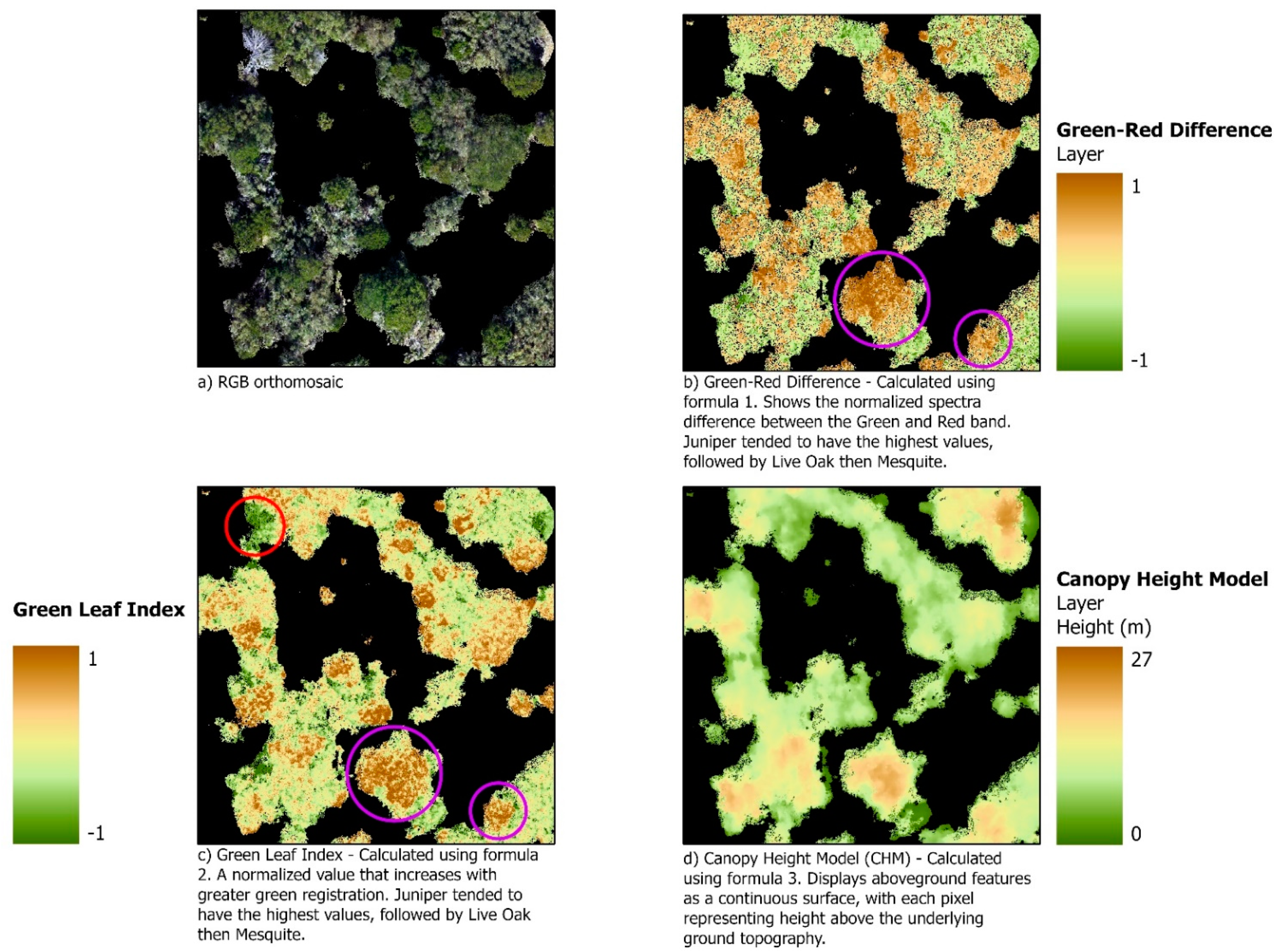
Additional information layers, as seen in Figure 3, were created by means of feature engineering; these were used for the traditional and machine learning classification but left out of the VGG-19 CNN classification to highlight the exceptional capability of the CNN to detect complex class patterns from standalone RGB imagery. For the particular camera used, the blue channel has a response curve of 400–560 nm with a peak at 460 nm, the green channel has a response curve of 400–640 nm with a peak at 540 nm, and the red channel has a response curve of 400–700 nm with a peak at 580 nm. These additional information bands were created via the following formula:
G r e e n R e d   D i f f e r e n c e = ( G R ) / ( G + R )  
G r e e n   L e a f   I n d e x = ( 2 × G R B ) / ( 2 × G + R + B )  
C a n o p y   H e i g h t   M o d e l   ( C H M ) = D S M D T M
where G = green wavelength (peak response at 540 nm); R = red wavelength (peak response at 580 nm); and B = blue wavelength (peak response at 460 nm).
The three features were selected for different purposes. The green–red difference and chlorophyll features distinguish more finely between the various levels of greenness between tree species [26], while the canopy height model (CHM) detects differences in the height of woody plants. The three features were stacked along with the RGB bands, creating a six-band dataset, and can be seen in Figure 3. The stacked data file was then resampled from 2.45 cm to 5 cm, at 10 cm, and at 15 cm to reduce the size of the data. Using image interpretation based on the presence of mixed pixels, the ability to accurately identify tree species, and overall image quality, we selected the resampled 10 cm mosaic for classification. Lastly, a simple decision tree classifier was used to mask out CHM values under 0.5 m for the majority of pixels representing ground properties and small herbaceous species. A similar step was carried out in [27] using a CHM to mask out values over 1 m to mask out tree species. For our site, a 1 m mask was unnecessary as the terrain is generally flat and many of the herbaceous species are shorter than 50 cm; furthermore, using a 1 m mask would have concealed a large number of young trees that should have been included in the classification.

2.3. Species Classification Using Traditional and Classical Machine Learning Methods

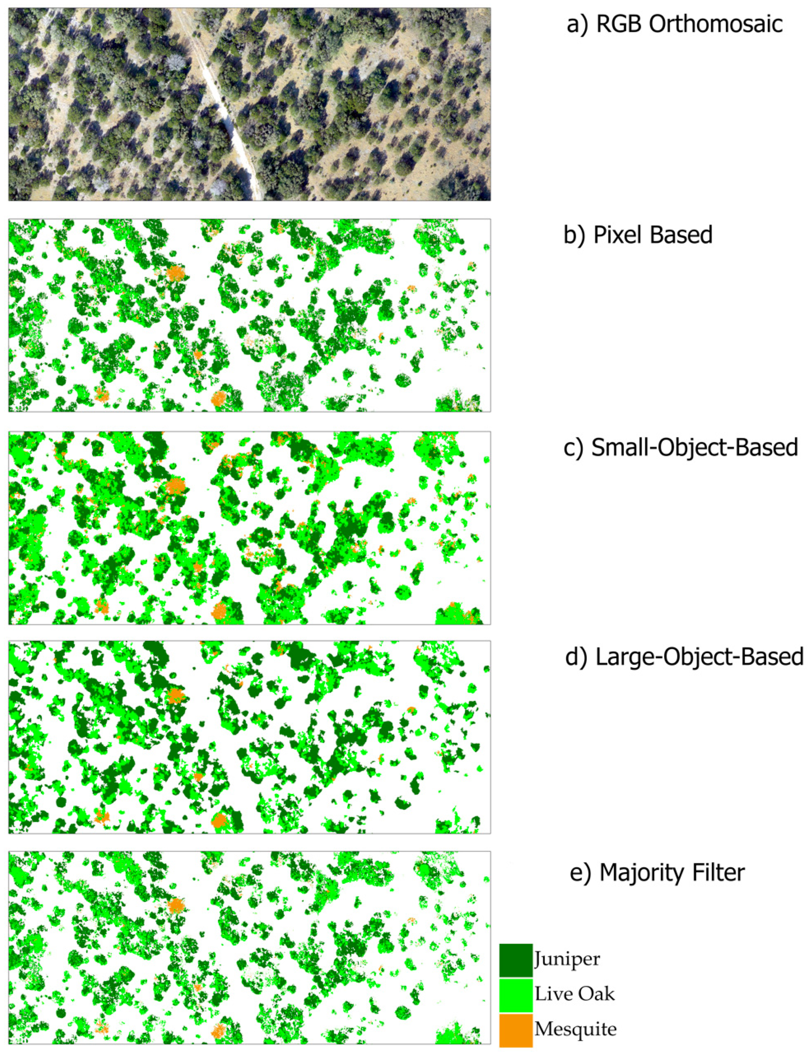
The classification scheme we selected included five classes: ground, shadow, juniper (both blueberry and redberry species), live oak, and mesquite. The shadow class was included to distinguish dark void areas from tree canopies and dark green junipers (most shadows cast on open ground were removed by the CHM mask). The ground class was included for the same reason—to distinguish among sunlit void areas, tree canopies live oaks, and leaf-off mesquites. Classification accuracy was assessed for the following five methodologies: (1) pixel-based classification with ML, SVM, and RF; (2) small-object-based classification with ML, SVM, and RF; (3) large-object-based classification with ML, SVM, and RF; (4) pixel-based classification with a post-processing majority filter; and (5) VGG-19 CNN deep learning classification.
For the training data, we selected 600 pixels per class on the 10 cm six-band orthomosaic, on the basis of the key characteristics for training area datasets listed in [28] as well as an expert understanding of the landscape and image analysis. We evaluated the separability of the collected training data based on the Jeffries–Matusita distance, which calculates interclass separability using the different spectral and physical band statistics used in the training area dataset. The range of values produced by this method is 0.0–2.0, with a score of 1.9 or better being ideal [29]. The J–M distance was calculated via the following formulas:
J _ x y = 2 ( 1 e B ) ,  
B = 1 / 8   ( ( x y ) ^ t   ) * ( ( Σ x + Σ y ) / 2 ) ^ ( 1 ) * ( x y ) + ( 1 / 2   l n ( ( | ( Σ x + Σ y ) / 2 ) | )   /   ( | Σ x | ^ ( 1 / 2 ) | Σ y | ^ ( 1 / 2 ) ) ) )   ,
where x is the vector of first-class spectral response; y is the vector of second-class spectral response; Σx= covariance matrix of sample x; and Σy= covariance matrix of sample y.
The J–M distance between all classes was greater than 1.9 except between juniper and live oak. The result for the latter two was expected because of their similar heights and spectral components (Table 1). A dendrogram, commonly used to hierarchically cluster taxa or classes, yielded results similar to those of the separability report—showing a close similarity between the juniper and live oak classes due to their spectral and physical similarities (Figure 4). In contrast, the J–M distance between classes, such as mesquite and shadow, which have very different spectral signals, was large.
Ideally, for testing data to ensure unbiased assessments of the accuracy of our classification results, in situ ground reference test pixels would have been collected [30]. However, because these were not available, we instead used visual interpretation of the original 2.45 cm raw images in combination with expert knowledge of the landscape and the tree species as a basis for collecting testing data on our 10 cm stacked orthomosaic (this method has been verified as a viable alternative for ground reference test information) [31]. We calculated the number of total testing pixels using the following formula [32] (p. 137):
N = B 4 b 2  
where N = number of testing samples; B = the upper (α/k) × 100th percentile of the chi square (χ2); and b = the desired precision.
The formula requires a minimum of 757 total testing pixels, but having 5 classes, we decided to select 1000 testing pixels, 200 for each class. We therefore generated 5000 random pixels across the orthomosaic, which were reduced to 200 pixels for each class, evenly distributed across the image (avoiding mixed pixels and class boundaries).

2.3.1. Image Segmentation

To enable comparisons between pixel-based and object-based approaches in classifying species, we carried out two separate segmentations in ESRI ArcMap®. The specific segmentation algorithm used was mean shift, which works by moving a window to fit around the center of a centroid placed in an area of maximum pixel density. ArcMap’s implementation of the mean shift segmentation segments the images on the basis of maximum object size, spectral detail (ranging from 0 to 20) and spatial detail (ranging from 0 to 20). We performed parameterization iteratively, using varying values and visually interpreting the results. The final two segmentations contained the same spectral and spatial detail parameters of 17. The first segmentation limited object size to a minimum of 10 pixels (referred to as small-object-based classification because it consists of only the smallest discernable objects). The second segmentation limited object size to a minimum of 100 pixels (referred to as large-object-based classification because it was the largest setting possible without taking in a large number of mixed class objects). Figure 5 illustrates the two segmentations.

2.3.2. Image Classification

We applied support vector machines, random forest, and maximum likelihood algorithms to classify species over our study site using both pixel-based and object-based methodologies. The support vector machines algorithm [33] is a nonparametric method that does not rely on training data normality or any assumptions regarding the underlying distributions of the training data but is designed to find the optimal hyperplane that separates the training dataset into discrete predefined classes [34]. The random forest algorithm [35] is an ensemble classifier that combines a number of decision trees (the number set by the user); these decision trees split at nodes on the basis of a random subset of predictors—the result being the sum of the majority votes from all the individual decision trees. The maximum likelihood algorithm was chosen due to its popular use in analyzing remotely sensed images and reliability in classifying a variety of cover types and conditions [36]. It works by using training data to determine class-specific mean vectors and variance–covariance matrices, producing probability density functions. The density functions are used to calculate the probability of every pixel in an image belonging to each predetermined class, with the highest computed class probability being assigned to the output classification image.
We used the ML, SVM, and RF algorithms for standard pixel-based classification on the stacked orthomosaic and performed parameter tuning for the ML, SVMs, and RF algorithm by cross-validation on three unique subsamples of the training data (accounting for 10%, or 60 pixels, for each class) and visually assessed the results.
For the final ML classifications, no probability threshold was set in order to classify every pixel, and the data scaling factor was set to 1023 based on a 10-bit radiometric resolution provided by our camera sensor.
The final SVM classifications used a radial basis function kernel whose value depends strictly on the separation between an input pixel and the hyperplane separating the information classes. The gamma value was set to 0.091, which decides the curvature of the separating hyperplane, with higher values resulting in greater curvature and a tighter fit around the data values, and a penalty parameter of 100, which balances the trade-off between training errors and forcing rigid margins. Increasing the penalty parameter increases the effect misclassified points have on the hyperplane, which can lead to overfitting.
The final RF classifications used 1000 decision trees, with each tree simulating a random vector sampled from the training data with the same distribution. Each tree consisted of a max tree depth of 50, which caps the number of decision nodes needed before casting a vote for the output classification image.
A majority filter was applied to the resulting classified images, by means of a 3 × 3 kernel moving across the image at a 1-pixel step interval. For replacement to occur, the neighboring pixels surrounding the central pixel must have a simple class majority and be contiguous around the center of the filter kernel to minimize the corruption of cellular spatial patterns.
We also applied object-oriented classification to the two segmented images (small- and large-object segmentations) using ML, SVM, and RF algorithms. The same parameters applied to each algorithm in the pixel-based classification were applied to both the small- and large-object segmented images.

2.4. Species Classification Using a Deep Learning Method

A variety of deep learning convolutional network (CNN) models have been proposed for various environmental applications, including object detection and semantic segmentation. Popular ones include VGG [37], Resnet [38], Inception V3 [39], and Xception [40]. The main advantage of deep learning CNNs over classical machine learning models lies in their feature engineering, scalability, and high performance. In this study, we evaluated the VGG-19 CNN due to its popular use in remote sensing applications and excellent results [41,42,43,44].

2.4.1. VGG-19 Model Overview

Developed in 2014, VGG-19 has proven over the years to be a competitive deep learning model when tasked with classifying land cover and tree species classes from remotely sensed images [41,42,43,44]. The VGG-19 CNN algorithm uses a SegNet encoder–decoder architecture, whereby the encoding CNN learns relevant, low-level features about the target class from the received RGB image and passes the information on to the decoder, which formulates a prediction using max pooling indices for every pixel in the RGB image. Specifically, the VGG-19 CNN takes 224 × 224 RGB input images and moves them through 19 weighted convolutional layers with a fixed-kernel filter of 3 × 3 and a stride of 1 pixel. Within every convolutional layer, each neuron/pixel is connected to a few nearby neurons/pixels in the previous layer, with the exact same set of weights used for each local connection. This process enhances the capability of the model to identify local features, uninfluenced by pixels across the image; and it also provides an equal chance for features to be detected anywhere throughout the image. At the end of each convolutional stack, the volume size is reduced by a fixed-kernel filter of 2 × 2 with a stride of 2 max pooling layers, which highlights the most obvious feature (largest value) in the patch. The stack of convolutional layers is followed by three fully connected layers, such that each neuron in a layer is connected with every neuron in the previous layer with its own weight. Lastly, a softmax layer normalizes the output of the network to a probability curve comprising the predicted output classes for each pixel.

2.4.2. Training Label Collection

Collecting training samples for the VGG-19 semantic segmentation method required a different approach. Rather than single pixels being collected, sample images with all pixels labeled with one of the five classes were created from full drone scenes. For labeling convenience, 50 512 × 512-pixel images were labeled in MATLAB® Image Labeler application. The images covered a total of 635m2, including 127 junipers, 103 live oaks, and 36 mesquites (appropriately representing each tree species’ relative abundance in our study area). To create a training set for model fitting, we subsampled each of the 50 images to randomly select 1000 224 × 224 images. Figure 6 shows sampled labeled data.

2.4.3. VGG-19 Model Training

We trained the VGG-19 model within the MATLAB programming environment using the computer vision and deep learning toolboxes. Since the VGG-19 model is a pretrained model, our training process was in essence an adaption of the model to new classes which it was not originally trained on, often referred to as transfer learning. Prior to training, the collected data, comprising the 1000 raw 224 × 224 RGB images and their associated labeled images, were split into training (75%) and validation (25%) sets. We then set up the training process in MATLAB by specifying the input training and validation data, the required input size (224 × 224), the pretrained model (VGG-19) and the number of semantic classes (in our case, 5). Considering the unbalanced sampling across the five semantic classes, weights were incorporated, calculated as the inverse frequency of each class, to strengthen the robustness of our model. Furthermore, to enhance the accuracy of the network, we then augmented the training data by randomly shifting, rotation, and reflecting them to create different versions of the data [45,46]. With a fully specified model, we trained it using mini batch stochastic gradient descent with momentum (SGDM) as the optimizer with 75% of the labeled data and 25% of the data for validation. Learning parameters, including schedule type, rate, factor, and mini batch size, followed the inputs set by [47]. Model training was accomplished over 100 epochs on a 64-bit Dell Workstation (Intel® Xeon® Processor with 256 GB RAM, NVIDIA™ Quadro K5200 GPU with 8 GB RAM) and took about 2 days to complete. Once model training was completed, we applied it to the 10cm RGB orthomosaic to generate a field-level classification map.

2.5. Accruacy Assessment

For consistency, the accuracy of each methodology was tested by producing an error matrix using the same 1000-point testing data set. These error matrices include both overall accuracies (OA) and kappa coefficients (KC), which were calculated using the following formulas:
O A = T C / N  
K C = N i 1 r x i i   i 1 r ( x i + X x + 1 ) / N 2 i 1 r ( x i i X x + 1 )     ,
where TC = total number of correctly labeled pixels, N = total number of testing pixels, r = number of rows and columns in the confusion matrix, Xii = observation in row i and column i, Xi+ = marginal total of row i, and X + I = marginal total of column i. OA and KC are standard metrics for assessing image classification accuracy, with the OA quantifying the accuracy of the entire product and the KC serving as a more robust measure that takes into account the probability of chance agreements.
We also included user (UA) and producer (PA) accuracies in our accuracy assessments to provide a more encompassing evaluation of the quality of our products. The UA refers to the point of view of the user who plans on using the classified map. It is defined as the probability that a classified pixel is in fact the class it says it is. The PA refers to the point of view of the map maker. It is defined as the probability of real features on the ground being correctly shown on the classified map. They were calculated using the following formulas:
U A = A / B  
P A = A / C  
where A = the number of pixels correctly identified in a given map class, B = the total number of pixels claimed by the map to be in that class, and C = total number of pixels in the reference class.

3. Results

Our assessments of accuracy for the five classification methodologies (pixel-based, small-object-based, large-object-based, pixel-based with a post-processing majority filter, and VGG-19 CNN) showed accuracies ranging from 77.1% to 96.9% (Table 2). The highest accuracy was achieved by the VGG-19 CNN deep learning methodology with an OA of 96.9% and a KC of 96.1%. The lowest accuracy was recorded for the large-object-based ML methodology with an OA of 77.1% and KC of 71.4%. Aside from these two methodologies, every method–algorithm combination attained an OA and KC between 85 and 94%, definitively showing that affordable RGB drone imagery is indeed capable of classifying woody plant species encroaching on semiarid grasslands and savannas.

3.1. Species Classification Using Traditional and Classical Machine Learning Methods

The non-post-processing pixel-based and large-object-based classification methodologies in combination with the ML and RF algorithms were found to be the least accurate (both showed OAs below 90%). On the other hand, both the small-object-based method and the pixel-based method with the post-processing majority filter showed OAs of over 90% for all three algorithms (the majority filter method performing slightly better for each algorithm). Further, regardless of the methodology used, the SVM algorithm outperformed both RF and ML and was the only algorithm that achieved a 90% accuracy for the large-object-based method. Figure 7 shows a subsection of the ML, RF, and SVM classifications, and Figure 8 illustrates the four methodologies in combination with SVM.
Producer accuracy (PA) and user accuracy (UA) were highest for the ground, shadow, and mesquite classes, with many in the mid-90% range (Table 3). The lowest PAs and UAs were seen for the live oak and juniper classes, with most falling below 90% for most methods and algorithms. The lowest UAs were found for the juniper class via large-object-based methodology (68.6% with RF and 63.8% with ML).

3.1.1. Pixel-Based Classification

The pixel-based method produced the best results when classified using SVM, attaining an OA of 90.4% and KC of 87.8%. ML outperformed RF when using a pixel-based approach with an OA of 88.2% to 87.3% and a KC of 85.3% to 84.1%. UAs and PAs were high for the ground, shadow, and mesquite class with averages above 90% among the three algorithms tested. However, the UA and PA for the juniper and live oak class were significantly lower. The UAs for the juniper class in particular were low, with accuracies below 80%. Furthermore, the PAs for the live oak class in particular were low, with only ML producing an accuracy above 80%. Overall, the results were acceptable but displayed a heavy salt-and-pepper effect that can be attributed to the high spatial resolution.

3.1.2. Small-Object-Based Classification

The small-object-based method produced similar results for SVM, RF, and ML with OAs and KCs of 90.1%/ 88.9%, 90.5%/ 88.1%, and 90.2%/ 87.8%, respectively. In comparison to the pixel-based method, the small-object-based method had more consistent UA and PA accuracies for all the classes. Specifically, only the UA for the juniper class using ML produced an accuracy of less than 80%. Overall, the results are comparable to those produced by the pixel-based method, including the salt-and-pepper effect, which was still present.

3.1.3. Large-Object-Based Classification

The large-object-based method produced high accuracies for SVM and RF with OAs and KCs of 90.3%/ 87.9%, and 88.5%/ 85.63%, respectively. ML accuracy dropped significantly with an OA and KC of 77.1% and 71.4%. Interestingly for SVM, the juniper class outperformed all other methods for PA and UA, both with accuracies above 90%. Conversely, ML had its lowest UA and PA with accuracies in each class below 80%. This highlights the robustness that classical machine learning algorithms (SVM, RF) have over traditional algorithms such as ML. Furthermore, this methodology greatly decreased the salt-and-pepper effect, allowing the user to better visualize species-specific tree crowns.

3.1.4. Pixel-Based Classification with a Post-Processing Majority Filter

The pixel-based classification with a post-processing majority filter produced the highest OAs and KCs for the traditional and classical algorithms, with the highest accuracy attained in combination with SVM (OA: 93.8% and KC: 92.3%). Additionally, UA and PA for all three algorithms and across each class never dropped below 80%, attaining the highest percentages for any method. Overall, this method provides an advantage in increased accuracies but retains a prominent salt-and-pepper effect that hinders interpretability of the classification map. This could possibly be mitigated by using larger filter windows, which may also change accuracies.

3.2. Species Classification using a Deep Learning Method

The VGG-19 CNN deep learning methodology, which can be seen in Figure 9, produced the highest accuracies across all methodologies with an OA of 96.9% and a KC of 96.1% (Table 4). All PA and UA values were well above 90%, with tree species classes achieving values in the mid-to-high 90% range (Table 5). This methodology, though highly accurate, requires a suitable GPU to train the model. Furthermore, labeling training data is a lengthy process, and parameterization of the model takes an increased level of expertise that may limit its usability. For these reasons, it would not be recommended to land managers as the primary methodology for classification.

4. Discussion

All the methodology and algorithm combinations we assessed achieved acceptable results, demonstrating that RGB images captured by drone can be used to accurately map woody plant species in semiarid regions. The VGG-19 CNN model achieved the highest overall accuracy (96.9%). SVM came in second with an average classification accuracy of 91.2% across all methods, followed by RF (89.7%) and ML (86.8%). The increased spatial resolution due to the low altitude of the flight, along with the innate differences among the woody species in seasonality and spectral qualities, creates a unique situation in the Edwards Plateau—such that accurate classification is possible only with bands in the visible spectrum. Acquiring imagery in December, when mesquites are leaf-off, live oaks begin to lose color, and junipers are fully leafed, takes advantage of conditions of stark contrast between the species. However, acquiring imagery in early March, when live oaks are thinning out and going through a short period of leaf senescence while mesquites have yet to regrow their leaves, might yield similar or possibly better results—particularly in distinguishing between live oaks and junipers in dense, multistoried canopies.

4.1. Object-Based vs. Pixel-Based Classification

Object-based classification is generally thought to be a better method than pixel-based classification, as it greatly reduces the salt-and-pepper effect seen in many pixel-based classification images. In [48], using ML on terra advanced space-borne thermal emission and reflection radiometer (ASTER) imagery for vegetation classification in northern California, the authors compared pixel-based image analysis and object-based analysis and found that the latter dramatically outperformed the former (83.25% to 46.48%). Similarly, when [49] used a multitude of traditional classification algorithms to compare object-based and pixel-based methods for classifying agriculture crops in southern Spain, they found that the accuracies of object-based classifications were on average 4% higher than their pixel-based counterparts. Unlike the results found in study [23], which concluded that a pixel-based approach was better in classifying woody encroachment into grasslands, we found that object-based approaches performed better when properly segmented, as well as providing a better outline of canopies. Finally, Ref. [50] used QuickBird imagery to classify urban land cover in central Phoenix, Arizona and found that object-based classification outperformed pixel-based classification in overall accuracy (90.4% to 67.6%). The findings of our study are similar, with small-object-based classification achieving better results than pixel-based classification, but the margins were not as large as those reported in other studies; overall accuracies with the ML, RF, and SVM algorithms were higher by 2%, 2.9%, and 0.7%, respectively. Increasing the maximum pixel size per object from 10 to 100 caused a decrease of 11.2% for ML and a decrease of 0.1% for SVM, while the overall accuracy for RF increased by 1.2%. These results display the robust ability of SVM to provide an accurate classification regardless of the method used. Algorithm-specific hyper-parameterization can be used to find the optimal maximum object size, but this was not the primary concern of our study. The decrease in ML classification accuracy is notable but expected given the underlying assumptions in maximum likelihood classification. At the larger object size, there was a higher chance of creating objects with mixed spectra, which likely violated the underlying normality assumptions.

4.2. Post-Processing Application

The use of a majority filter for post classification smoothing on the pixel-based classification outputs resulted in the highest overall accuracies for the ML, RF, and SVM algorithms, which were greater by 3.4%, 5%, and 3.4%, respectively, than those achieved via standard pixel-based or object-based classification. The authors of [51], using Landsat thematic mapper imagery and topographic data, classified land cover classes with the RF algorithm and found that post classification smoothing increased overall accuracy results by up to 6%. Our accuracy improvements were not as great, which is most likely due to the large difference in spatial resolutions (0.1 m vs. 30 m). However, it is important to note that even though the majority filter produced the highest overall accuracies for ML, RF, and SVM, there was still a considerable salt-and-pepper noise associated with the classification. The salt-and-pepper effect, due to the increased spatial and radiometric resolution provided by drones, was greatly reduced for the small-object-based and large-object-based classifications, with the large-object-based classification producing the clearest outlines of tree canopies, as illustrated in Figure 8.

4.3. Tradional vs. Classical Machine Learning Classification

Both machine learning algorithms, SVM and RF, outperformed the traditional ML algorithm with all the methodologies, the exception being that with the pixel-based method, ML had a 0.9% greater overall accuracy than RF. Overall, SVM performed better than RF and ML across the board, which was to be expected; the SVM algorithm is generally claimed to be the best at dealing with classifications of higher information classes such as woody plant species, with the RF algorithm coming second [52,53]. Further, the SVM was also the most robust of the three algorithms, yielding accuracies above 90% with all the methodologies. This robustness can be explained by its non-parametric nature, which enables it to properly find an optimal class-separating hyperplane, regardless of the number of training samples used or their inherent variability and number of outliers [54].

4.4. Deep Learning Application

It was the fourth algorithm assessed, the VGG-19 CNN algorithm, that achieved the highest overall classification accuracy, as well as the highest average per-class accuracy, for the woody plant species at 96.9%. This greater accuracy can be attributed to both the number of training data used to train the model, and the quality of the training data. For deep learning algorithms, every pixel in the image must be labeled, which requires detailed knowledge of the study area. Thus, labeling training data can be an arduous process, and deep learning model training can be lengthy. However, data augmentation techniques, such as rotation, mirroring, and splicing, enable a larger number of high-quality training samples to be produced [40,41].
Other CNN architectures have been widely used in solving classification problems from remotely sensed images; however, VGG-19 remains a strong competitor for such tasks. In 2021, [42] applied pretrained models, InceptionV3, Resnet50V2, and VGG-19, to LCLU classification in the UC Merced dataset, resulting in accuracy performances of 92.46, 94.38, and 99.64%, respectively. Within the same year, [43] implemented a pretrained VGG-16 model (same architecture as VGG-19 with three fewer convolutional layers) for LULC classification using the RGB version of the EuroSat dataset, achieving an accuracy of 99.17%. In 2019, [44] gathered a combination of LiDAR and high-resolution RGB data by plane to classify 18 tree species in a tropical wetland forest using three deep learning models (i.e., AlexNet, VGG-16, and ResNet50). VGG16 outperformed the other two models, scoring the highest overall classification accuracy of 73.25%. Studies [20,21,22], which used various CNNs to classify tree species in humid climates and urban areas, garnered similar results to ours, showing that the combination of deep learning and high-resolution drone imagery can provide high classification accuracies in other landscapes as well. Testing other deep learning models in semiarid woody encroached landscapes would provide useful information; however, it is out of the scope of this study, as we simply wanted to test the efficacy of using affordable RGB drone data to identify encroaching woody plant species and develop recommendations based on our results.

4.5. Recommendation

We recommend a large-object-based SVM classifier when classifying woody plant species in semiarid grasslands and savannas from drone imagery. This methodology did not produce the highest overall accuracy but had exceptional results nonetheless, with an OA above 90%. It also classified juniper, the most abundant species in our study area, with a higher degree of accuracy than the other non-deep learning methodologies. Furthermore, using SVM in combination with large-object-based classification allowed us to clearly visualize tree crowns. Lastly, gathering training data and processing times were also much faster when compared to properly training and applying the VGG-19 CNN to the orthomosaic.

5. Conclusions

Our findings show that RGB drone sensors are indeed capable of providing highly accurate classifications of woody plant species in semiarid landscapes—comparable to and even greater in some regards to those achieved by aerial imagery using hyperspectral sensors in more diverse landscapes. One reason for the high quality of the classifications we were able to obtain could be the innate seasonal diversity of the woody plant species found in the semiarid Edwards Plateau. Using drones enables continuous surveillance of an area, with little preflight planning required. This advantage over using aerial or satellite imagery means that land managers and scientists can more easily investigate site-specific and species-specific problems, including the woody plant encroachment that has seriously affected many such areas.
The best overall accuracies are achieved by pairing drone imagery with a deep learning, convolutional neural network algorithm, such as VGG-19, which can be replicated with the labeling of new images every time new data are gathered. However, the tedious nature of labeling a large number of training samples, GPU requirements, and long model training times makes this method difficult to implement. For this reason, further studies in these landscapes should be undertaken to test other deep learning models to see which performs best and to train models with smaller samples of training data to see how accuracies and processing times are affected. Testing of different models and of varying numbers of training data is needed to find a balance between long processing times and acceptable classification accuracies. Another avenue that would add to our knowledge base would be to gather data during summer months, when all the wood plant species are in full bloom, to gain insights into possible limitations of RGB drone imagery in these landscapes. Additionally, yet another avenue for increasing our understanding of the capability of high-resolution RGB drone imagery would be to perform similar studies in other semiarid grasslands and savannas regions of the world with a different variety of encroaching woody plant species.
An exciting future possibility would be to expand the study further through data fusion with National Agricultural Imagery Program (NAIP) imagery that provides country wide 1-meter ground sample distance every 3 years. Data fusion would allow for plot-level evaluation of woody plant encroachment to be applied across the entire Edwards Plateau region of Texas and other semiarid regions of the continental United States (CONUS). Additionally, NAIP imagery being acquired every 3 years allows us to track change, thereby mapping the spread of woody species across semiarid regions of the CONUS. Furthermore, NAIP imagery is publicly available on the Google Earth Engine (GEE) providing interested parties the ability to use Google’s powerful cloud computing capabilities.
Finally, our recommendation to those working in these landscapes is to use an object-oriented SVM classifier due to its ease of implementation, fast turnaround time, relatively high overall and tree class accuracy, and accurate depiction of tree crowns. This study provides important groundwork for such efforts by demonstrating that using RGB imagery captured by drones is a cost-effective and time-efficient strategy for classifying woody plant species in semiarid grasslands and savannas.

Author Contributions

Conceptualization, H.G.O. and S.C.P.; Methodology, H.G.O. and S.C.P.; Software, H.G.O., L.M., and C.V.; validation, H.G.O. and C.V.; formal analysis, H.G.O.; investigation, H.G.O., L.M., and S.C.P.; resources, L.M. and S.C.P.; data curation, L.M.; writing—original draft preparation, H.G.O.; writing—review and editing, H.G.O., B.P.W., L.M., and S.C.P.; visualization, H.G.O., S.C.P., and L.M.; supervision, S.C.P. and B.P.W.; project administration, S.C.P.; funding acquisition, N/A. All authors have read and agreed to the published version of the manuscript.

Funding

This research was provided by the Savanna Long-term Research and Education Initiative (SLTREI), Department of Ecology and Conservation Biology, Texas A&M University.

Acknowledgments

In this section, you can acknowledge any support given which is not covered by the author contribution or funding sections. This may include administrative and technical support, or donations in kind (e.g., materials used for experiments).

Conflicts of Interest

The authors declare no conflict of interest.

References

  1. Luvuno, L.; Biggs, R.; Stevens, N.; Esler, K. Woody Encroachment as a Social Ecological Regime Shift. Sustainability 2018, 10, 2221. [Google Scholar] [CrossRef] [Green Version]
  2. Eggemeyer, K.D.; Schwinning, S. Biogeography of woody encroachment; why is mesquite excluded from shallow soils? Ecohydrology 2009, 2, 81–87. [Google Scholar] [CrossRef]
  3. Wilcox, B.P.; Huang, Y. Woody plant encroachment paradox: Rivers rebound as degraded grasslands convert to woodlands. Geophvs. Res. Lett. 2010, 37, L07402. [Google Scholar] [CrossRef] [Green Version]
  4. Jessup, K.E.; Barnes, P.W.; Boutton, T.W. Vegetation dynamics in a Quercus-Juniperus savanna: An isotopic assessment. J. Veg. Sci. 2003, 14, 841–852. [Google Scholar] [CrossRef]
  5. Crustinger, G.M.; Short, J.; Sollenberger, R. The GUre of UAVs in Ecology: An Insider Perspective from the Silicon Valley Drone Industry. J. Unmanned Veh. Syst. 2016, 4, 161–168. [Google Scholar] [CrossRef] [Green Version]
  6. Wu, B.X.; Redeker, E.J.; Thurow, T.L. Vegetation and Water Yield Dynamics in an Edwards Plateau Watershed. J. Range Manag. 2001, 54, 98–105. [Google Scholar] [CrossRef]
  7. Huang, C.; Davis, L.S.; Townshend, J.R.G. An assessment of support vector machines for land cover classification. Int. J. Remote Sens. 2002, 23, 725–749. [Google Scholar] [CrossRef]
  8. Khatami, R.; Mountrakis, G.; Stehman, S.V. A meta-analysis of remote sensing research on supervised pixel-based land cover image classification processes: General guidelines for practitioners and future research. Remote Sens. Environ. 2016, 177, 89–100. [Google Scholar] [CrossRef] [Green Version]
  9. Fassnacht, F.E.; Latifi, H.; Sterenczak, K.; Modezelewska, A.; Lefsky, M.; Waser, L.T.; Straub, C.; Ghosh, A. Review of studies on tree species classification from remotely sensed data. Remote Sens. Environ. 2016, 186, 64–87. [Google Scholar] [CrossRef]
  10. Sheykhmousa, M.; Mahdianpari, M.; Ghanbari, H.; Mohammadimanesh, F.; Ghamisi, P.; Homayouni, S. Support Vector Machine versus Random Forest for Remote Sensing Image Classification: A Meta-Analysis and Systematic Review. IEEE J. Sel. Top. Appl. 2010, 13, 6308–6325. [Google Scholar] [CrossRef]
  11. Belgiu, M.; Dragut, L. Random forest in remote sensing: A review of applications and future directions. ISPRS J. Photogramm. 2016, 114, 24–31. [Google Scholar] [CrossRef]
  12. Heydari, S.S.; Mountrakis, G. Effect of classifier selection, reference sample size, reference class distribution and scene heterogeneity in per-pixel classification accuracy using 26 Landsat sites. Remote Sens. Environ. 2018, 204, 648–658. [Google Scholar] [CrossRef]
  13. Heydari, S.S.; Mountrakis, G. Meta-analysis of deep neural networks in remote sensing: A comparative study of mono-temporal classification to support vector machines. ISPRS J. Photogramm. Remote Sens. 2019, 152, 192–210. [Google Scholar] [CrossRef]
  14. Dalponte, M.; Bruzzone, L.; Gianelle, D. Tree species classification in the Southern Alps based on the fusion of very high geometrical resolution multispectral/hyperspectral images and LiDAR data. Remote Sens. Environ. 2012, 123, 258–270. [Google Scholar] [CrossRef]
  15. Raczko, E.; Zagajewski, B. Comparison of support vector machine, random forest and neural network classifiers for tree species classification on airborne hyperspectral APEX images. Eur. J. Remote Sens. 2017, 50, 144–155. [Google Scholar] [CrossRef] [Green Version]
  16. Immitzer, M.; Atzberger, C.; Koukal, T. Tree Species Classification with Random Forest Using Very High Spatial Resolution 8-Band WorldView-2 Satellite Data. Remote Sens. 2012, 4, 2661–2693. [Google Scholar] [CrossRef] [Green Version]
  17. Adelabu, S.A.; Mutanga, O.; Adam, E.M.I.; Cho, M.A. Exploiting machine learning algorithms for tree species classification in semiarid woodland using RapidEye image. J. Appl. Remote Sens. 2013, 7, 073480. [Google Scholar] [CrossRef]
  18. Paz-Kagan, T.; Chang, J.G.; Shoshany, M.; Sternberg, M.; Karnieli, A. Assessment of Plant Species Distribution and Diversity along a Climatic Gradient from Mediterranean Woodlands to Semi-Arid Shrublands. GIsci. Remote Sens. 2021, 58, 929–953. [Google Scholar] [CrossRef]
  19. Baena, S.; Moat, J.; Whaley, O.; Boyd, D.S. Identifying species from the air: UAVs and the very high resolution challenge for plant conservation. PLoS ONE 2017, 12, e0188714. [Google Scholar] [CrossRef] [Green Version]
  20. Onishi, M.; Ise, T. Explainable Identification and Mapping of Trees Using UAV RGB Image and Deep Learning. Sci. Rep. 2021, 11, 903. [Google Scholar] [CrossRef]
  21. Zhang, C.; Xia, K.; Feng, H.; Yang, Y.; Du, X. Tree Species Classification Using Deep Learning and RGB Optical Images Obtained by an Unmanned Aerial Vehicle. J. For. 2021, 32, 1879–1888. [Google Scholar] [CrossRef]
  22. Schiefer, F.; Kattenborn, T.; Frick, A.; Frey, J.; Schall, P.; Koch, B.; Schmidtlein, S. Mapping Forest Tree Species in High Resolution UAV- based RGB-Imagery by Means of Convolutional Neural Networks. SPRS J. Photogramm. Remote Sens. 2020, 170, 205–215. [Google Scholar] [CrossRef]
  23. Oddi, L.; Cremonese, E.; Ascari, L.; Filippa, G.; Galvagno, M.; Serafino, D.; Cella, U.M.D. Using UAV Imagery to Detect and Map Woody Species Encroachment in a Subalpine Grassland: Advantages and Limits. Remote Sens. 2021, 13, 1239. [Google Scholar] [CrossRef]
  24. Walker, B.H.; Ludwig, D.; Holling, C.S.; Peterman, R.M. Stability of Semi-Arid Savanna Grazing Systems. J. Ecol. 1981, 2, 473–498. [Google Scholar] [CrossRef]
  25. Fowler, N.L.; Dunlap, D.W. Grassland Vegetation of the Eastern Edwards Plateau. Am. Midl. Nat. 1986, 115, 146–155. [Google Scholar] [CrossRef]
  26. Louhaichi, M.; Borman, M.M.; Johnson, D.E. Located Platform and Aerial Photography for Documentation of Grazing Impacts on Wheat. Geocarto Int. 2001, 16, 65–70. [Google Scholar] [CrossRef]
  27. Van Iersel, W.; Straatsma, M.; Addink, E.; Middelkoop, H. Monitoring height and greenness of non-woody floodplain vegetation with UAV time series. ISPRS J. Photogramm. 2018, 141, 112–123. [Google Scholar] [CrossRef]
  28. Campbell, J.B.; Wynne, R.H. Image Classification. In Introduction to Remote Sensing, 5th ed.; Guilford Press: New York, NY, USA, 2011; pp. 350–355. [Google Scholar]
  29. Richards, J.A. Remote Sensing Digital Image Analysis, 5th ed.; Springer: Berlin, Germany, 2013; pp. 350–351. [Google Scholar]
  30. Jensen, R.J. Introductory Digital Image Processing, 4th ed.; Pearson: New York, NY, USA, 2015; pp. 500–504. [Google Scholar]
  31. Morisette, J.T.; Privette, J.L.; Strahler, A.; Mayaux, P.; Justice, C.O. Validation of Global Land-Cover Products by Committee on Earth Observing Satellites. In Geospatial Data Accuracy Assessment; Lunetta, R.S., Lyon, J.G., Eds.; EPA: Poquoson, VA, USA, 2004; p. 335. [Google Scholar]
  32. Congalton, R.G.; Green, K. Assessing the Accuracy of Remotely Sensed Data: Principles and Practices, 3rd ed.; Lewis Publishers: Boca Raton, FL, USA, 1999; p. 137. [Google Scholar]
  33. Vapnik, V.N. Statistical Learning Theory, 1st ed.; John Wiley and Sons, Inc.: Hoboken, NJ, USA, 1998. [Google Scholar]
  34. Mountrakis, G.; Im, J.; Ogole, C. Support Vector Machines in Remote Sensing: A review. ISPRS J. Photogramm. 2011, 66, 247–259. [Google Scholar] [CrossRef]
  35. Breiman, L. Random Forests. Mach. Learn. 2001, 45, 5–32. [Google Scholar] [CrossRef] [Green Version]
  36. Swain, P.H.; Davis, S. Remote Sensning: The Quantitative Approach; McGraw-Hill, Inc.: New York, NY, USA, 1978; p. 396. [Google Scholar]
  37. Simonyan, K.; Zisserman, A. Very Deep Convolutional Networks for Large-Scale Image Recognition. In Proceedings of the International Conference on Learning Representations, San Diego, CA, USA, 7–9 May 2015. [Google Scholar]
  38. He, K.; Zhang, X.; Ren, S.; Sun, J. Deep Residual Learning for Image Recognition. In Proceedings of the IEEE Conference on Computer Vision and Pattern Recognition, Las Vegas, NV, USA, 21–26 July 2016. [Google Scholar] [CrossRef] [Green Version]
  39. Szegedy, C.; Vanhoucke, V.; Loffe, S.; Shlens, J.; Wojna, Z. Rethinking the Inception Architecture for Computer Vision. In Proceedings of the IEEE Conference on Computer Vision and Pattern Recognition, Las Vegas, NV, USA, 21–26 July 2016. [Google Scholar] [CrossRef] [Green Version]
  40. Chollet, F. Xception: Deep Learning with Depthwise Separable Convolutions. In Proceedings of the IEEE Conference on Computer Vision and Pattern Recognition, Honolulu, HI, USA, 21–26 July 2017. [Google Scholar] [CrossRef] [Green Version]
  41. Yuan, Q.Q.; Shen, H.F.; Li, T.; Li, Z.; Li, S.; Jiang, Y.; Xu, H.Z.; Tan, W.W.; Yang, Q.Q.; Wang, J.; et al. Deep Learning in Environmental Remote Sensing: Achievements and Challenges. Remote Sens. Environ. 2020, 241, 111716. [Google Scholar] [CrossRef]
  42. Alem, A.; Kumar, S. Transfer Learning Models for Land Cover and Land Use Classification in Remote Sensing Image. Apppl. Artif. Intell. 2021, 1, 1–9. [Google Scholar] [CrossRef]
  43. Naushad, R.; Kaur, T.; Ghaderpour, E. Deep Transfer Learning for Land Use and Land Cover Classification: A Comparitive Study. Sensors 2021, 21, 8083. [Google Scholar] [CrossRef] [PubMed]
  44. Sun, Y.; Huang, J.; Ao, Z.; Lao, D.; Xin, Q. Deep Learning Approaches for the Mapping of Tree Species Diversity in a Tropical Wetland Using Airborne LiDAR and High-Spatial-Resolution Remote Sensing Images. Forests 2019, 10, 1047. [Google Scholar] [CrossRef] [Green Version]
  45. Shorten, C.; Khoshgoftarr, T.M. A Survey on Image Data Augmentation for Deep Learning. J Big Data 2019, 6, 1–48. [Google Scholar] [CrossRef]
  46. Yu, X.; Wu, X.; Luo, C.; Ren, P. Deep Learning in Remote Sensing Scene Classification: A Data Augmentation Enhanced Convolutional Neural Network Framework. Gisci. Remote Sens. 2017, 54, 741–758. [Google Scholar] [CrossRef] [Green Version]
  47. Malambo, L.; Popescu, S.; Ku, N.-W.; Rooney, W.; Zhou, T.; Moore, S. A Deep Learning Semantic Segmentation-Based Approach for Field-Level Sorghum Panicle Counting. Remote Sens. 2019, 11, 2939. [Google Scholar] [CrossRef] [Green Version]
  48. Gao, Y.; Mas, J.-F.; Maathuis, B.H.P.; Zhang, X.; Van Dijk, P.M. Comparison of Pixel-Based and Object-Oriented Image Classification ASpproaches—A Case Study in a Coal Fire Area, Wuda, Inner Mongolia, China. Int. J. Remote Sens. 2006, 27, 4039–4055. [Google Scholar] [CrossRef]
  49. Castillejo-Gonzalez, I.L.; Lopez-Granados, F.; Garcia-Ferrer, A.; Pena-Barragan, J.M.; Jurado-Exposito, M.; Sanchez de la Orden, M.; Gonzalez-Audicana, M. Object- and Pixel-Based Analysis for Mapping Crops and Their Agro-Environmental Associated Measures Using QuickBird Imagery. Comput. Electron. Agric. 2009, 68, 207–215. [Google Scholar] [CrossRef]
  50. Myint, S.W.; Gober, P.; Brazel, A.; Grossman-Clarke, S.; Weng, Q. Per-Pixel vs. Object Based Classification of Urban Land Cover Extraction Using High Spatial Resolution Imagery. Remote Sens. Environ. 2011, 115, 1145–1161. [Google Scholar] [CrossRef]
  51. Zhu, X. Land cover classification using moderate resolution satellite imagery and random forests with post-hoc smoothing. J. Spatial. Sci. 2013, 58, 323–337. [Google Scholar] [CrossRef]
  52. Ghosh, A.; Fassnacht, F.E.; Joshi, P.K.; Koch, B. A framework for mapping tree species combining hyperspectral and LiDAR data: Role of selected classifiers and sensor across three spatial scales. Int. J. Appl. Earth Obs. 2014, 26, 49–63. [Google Scholar] [CrossRef]
  53. Burai, P.; Deak, B.; Valko, O.; Tomor, T. Classification of herbaceous vegetation using airborne hyperspectral imagery. Remote Sens. 2015, 7, 2046–2066. [Google Scholar] [CrossRef] [Green Version]
  54. Camps-Valls, G.; Gomez-Chova, L.; Calpe, J.; Olivas, E.S.; Mart’in, J.D.; Alonso, L.; Moreno, J. Robustness Support Vector Method for Hyperspectral Data Classification and Knowledge Discovery. IEEE Trans. Geogsci. Remote Sens. 2004, 42, 1530–1542. [Google Scholar] [CrossRef]
Figure 1. The woody species that can be found in our study site and across the Edwards Plateau. (a) Live Oak (Quercus Virginiana) is a semi-evergreen woody plant that loses some of its greenness through the winter months. (b) Blueberry/Redberry Juniper (Juniperus ashei/pinchotti) is a perennial evergreen woody plant that remains green throughout the year. (c) Honey Mesquite (Prosopis Glandulosa) is a deciduous woody plant that loses its leaves through the winter months.
Remotesensing 14 01665 g001
Figure 2. Location of the study site. It covers a small portion of the southwest region of the Edwards Plateau ecoregion in the state of Texas, USA.
Remotesensing 14 01665 g002
Figure 3. The 3 data layers created to improve the traditional and classical machine learning classifications. (a) The 10 cm orthomosaic. (b) The Green-Red Difference layer only discerns junipers (displayed as dark brown). (c) The Green Leaf Index layer is able to discern the mesquites (displayed as dark green) and the juniper (displayed as brown). (d) The Canopy Height Model layer discerns the tops of individual woody plants with lighter green/brown and the edges of tree canopies as darker green.
Remotesensing 14 01665 g003
Figure 4. Dendrogram showing clustering and interclass distances for the five training classes.
Remotesensing 14 01665 g004
Figure 5. A display of the two segmentations performed on the orthomosaic. (a) The 10 cm orthomosaic. (b) The small-object segmentation limited object size to a minimum of 10 pixels, after which lowering the minimum size was deemed over-segmented. (c) The large-object segmentation limited object size to a minimum of 100 pixels, after which increasing the minimum size incurred a large number of mixed pixels.
Remotesensing 14 01665 g005
Figure 6. Labeled training images used to run the VGG-19 CNN. Images were carefully selected to accurately represent the class features in our study area. (a) A labeled image containing juniper and live oak, as well as some open area. (b) A labeled image containing a heavily forested scene with all three woody plant species. (c) A labeled image containing an open area, juniper, live oak, and large shadows.
Remotesensing 14 01665 g006
Figure 7. A comparison of the 3 traditional and classical machine learning algorithms used to classify the woody plant species in our study area. (a) The 10 cm orthomosaic. (b) ML tended to overestimate mesquite cover, as well as total tree cover with what was generally shadow. (c) RF was similar to ML, overestimating tree cover with shadow. (d) Overall, SVM was more robust in parsing between shadow and canopy cover for the three tree species.
Remotesensing 14 01665 g007
Figure 8. A comparison of the 4 methodologies (using SVM) employed to classify the woody plant species in our study area. (a) The 10 cm orthomosaic. (b) The pixel-based method provided decent accuracies but suffered from a strong salt-and-pepper effect (c) The small-object-based method attained better classification accuracies than the pixel-based method, while also providing a clearer representation of the landscape (d) The large-object-based classification most accurately depicted tree canopies; however, it lacked overall and class accuracies, due to a greater number of mixed pixels. (e) The post-classification majority filter attained the highest scores overall and class accuracies; however, it tended to underestimate total canopy coverage for all three woody plant species.
Remotesensing 14 01665 g008
Figure 9. The VGG-19 CNN classification map.
Remotesensing 14 01665 g009
Table 1. Class separability values using Jeffries–Matusita distance.
Jeffries–Matusita DistanceGroundShadowJuniperLive OakMesquite
Ground-1.99991.99991.95011.9515
Shadow1.9999-1.99831.99951.9977
Juniper1.99991.9983-1.88001.9996
Live Oak1.95011.99951.8800-1.9570
Mesquite1.95151.99771.99961.9570-
Table 2. Overall accuracies and kappa coefficients for the classical and traditional machine learning methods.
Overall Accuracy (%)Kappa Coefficient (%)
Pixel-BasedML88.285.3
RF87.384.1
SVM90.488.0
Small-Object-BasedML90.287.8
RF90.588.1
SVM90.188.9
Large-Object-BasedML77.171.4
RF88.585.6
SVM90.387.9
Majority FilterML91.689.5
RF92.390.4
SVM93.892.3
Table 3. User and producer accuracies for the traditional and machine learning methods.
Ground (UA/PA)(%)Shadow (UA/PA)(%)Juniper (UA/PA)(%)Live Oak (UA/PA)(%)Mesquite (UA/PA)(%)
Pixel-BasedML92.7/95.098.8/84.077.9/86.580.0/84.094.8/91.5
RF90.1/91.093.4/92.577.3/87.082.3/74.594.3/91.5
SVM93.7/96.595.9/94.079.0/90.086.7/78.098.4/93.5
Small-Object-BasedML92.2/89.097.8/90.593.9/85.075.0/94.597.4/92.0
RF89.9/93.591.5/96.586.7/88.085.9/85.599.4/89.0
SVM96.8/90.594.4/92.585.8/90.585.2/86.094.1/96.0
Large-Object-BasedML99.0/51.087.6/53.063.8/99.577.6/90.079.3/92.0
RF98.5/96.596.3/78.068.6/98.593.5/71.597.0/98.0
SVM97.2/70.597.5/97.090.2/97.075.9/91.595.5 /95.5
Majority FilterML95.1/96.098.9/86.081.7/93.588.4/87.596.5/ 95.0
RF94.0/93.594.0/94.584.8/95.093.8/82.596.0/96.0
SVM97.0/96.597.5/95.583.0/97.594.8/81.599.0/98.0
Table 4. Overall accuracies and kappa coefficients for the deep learning method.
Overall Accuracy (%)Kappa Coefficient (%)
Deep LearningVGG-1996.996.1
Table 5. User and producer accuracies for the traditional and machine learning methods.
Ground (UA/PA) (%)Shadow (UA/PA) (%)Juniper (UA/PA) (%)Live Oak (UA/PA) (%)Mesquite (UA/PA) (%)
Deep LearningVGG-1995.7/99.099.5/96.094.3/99.597.0/95.598.4/94.5
Publisher’s Note: MDPI stays neutral with regard to jurisdictional claims in published maps and institutional affiliations.

