
Modeling the CO


 , , and
Abstract
:1. Introduction
2. Model Description
3. Data Description
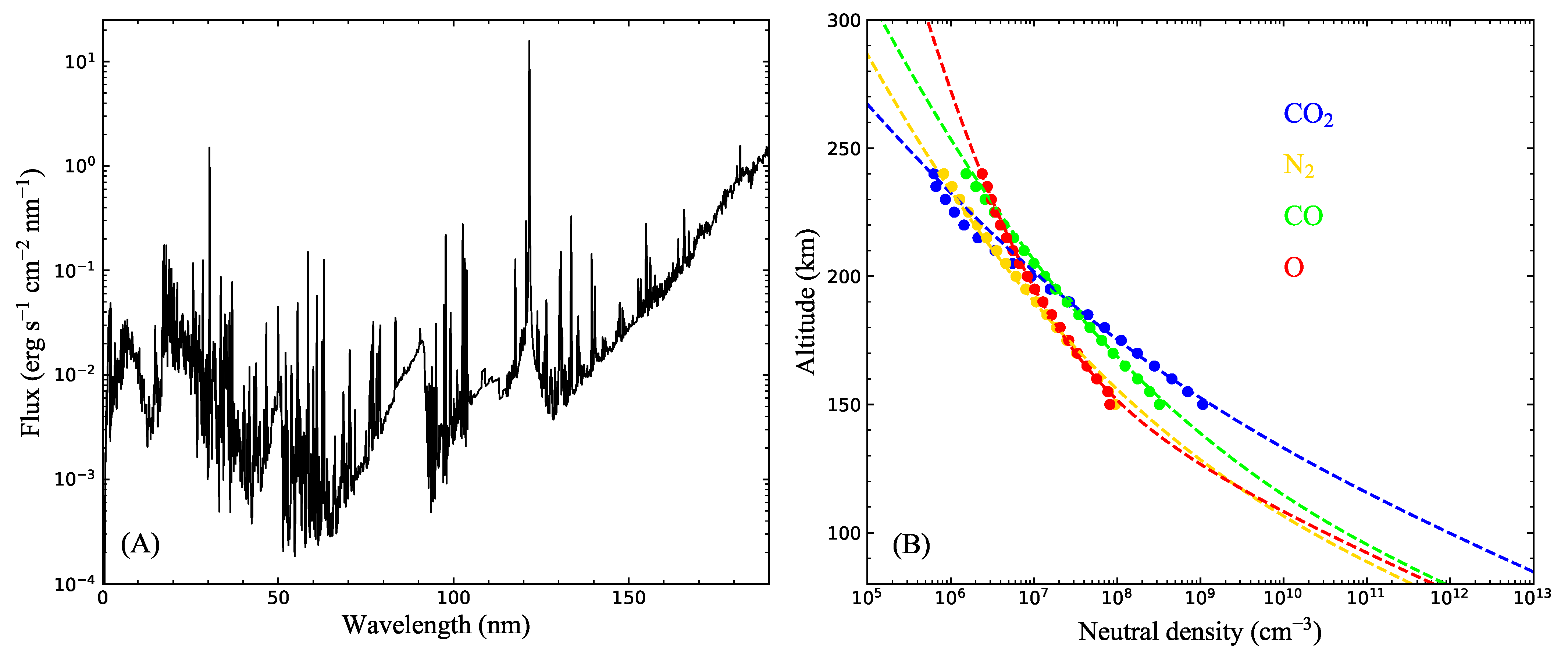
3.1. EUVM-Based Solar Flux
3.2. NGIMS-Based Neutral Density
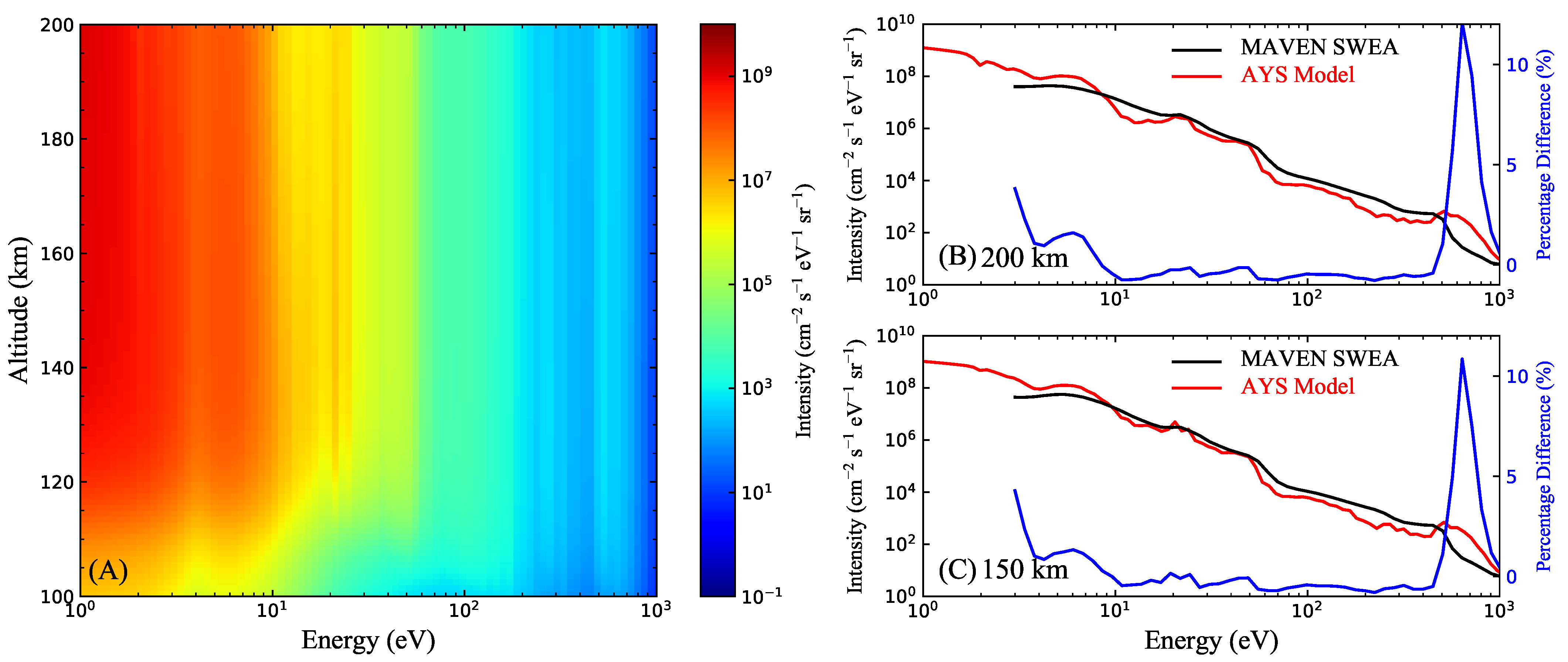
3.3. AYS-Based Photoelectron Intensity
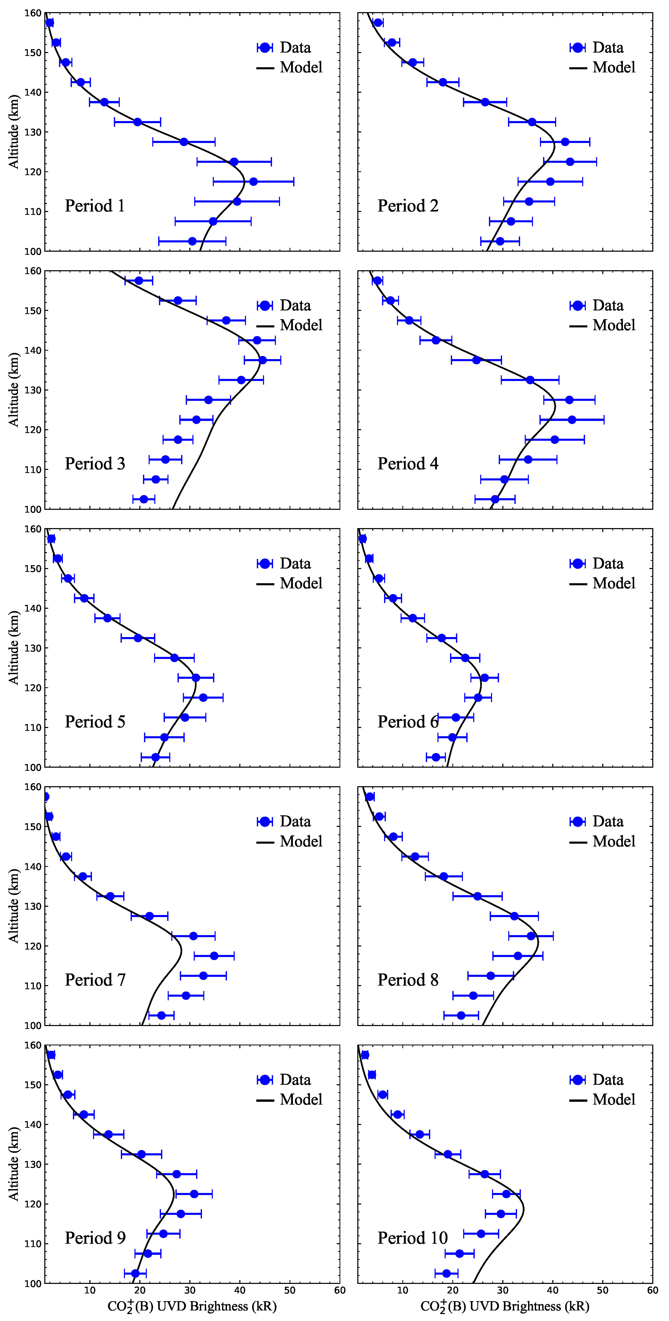
3.4. IUVS-Based CO UVD Emission
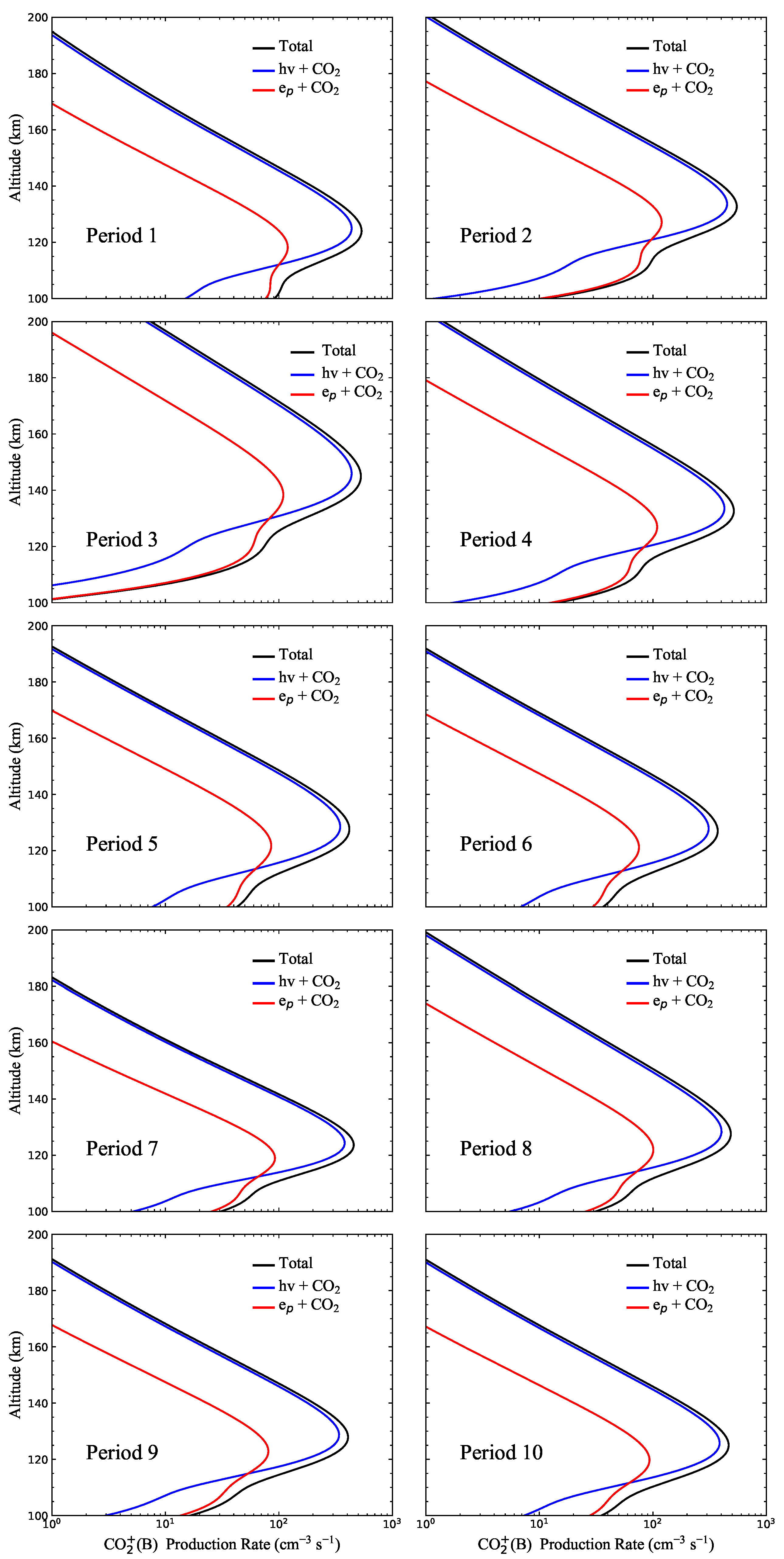
4. Model Results
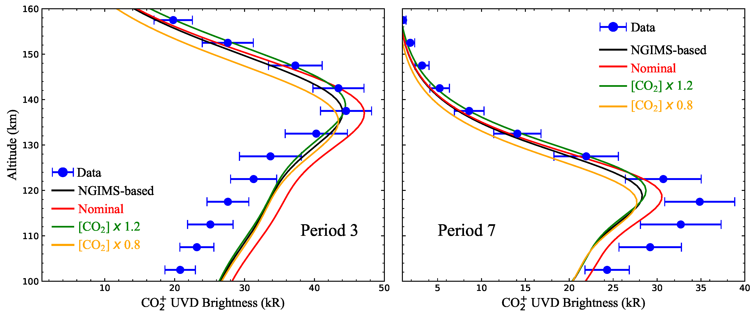
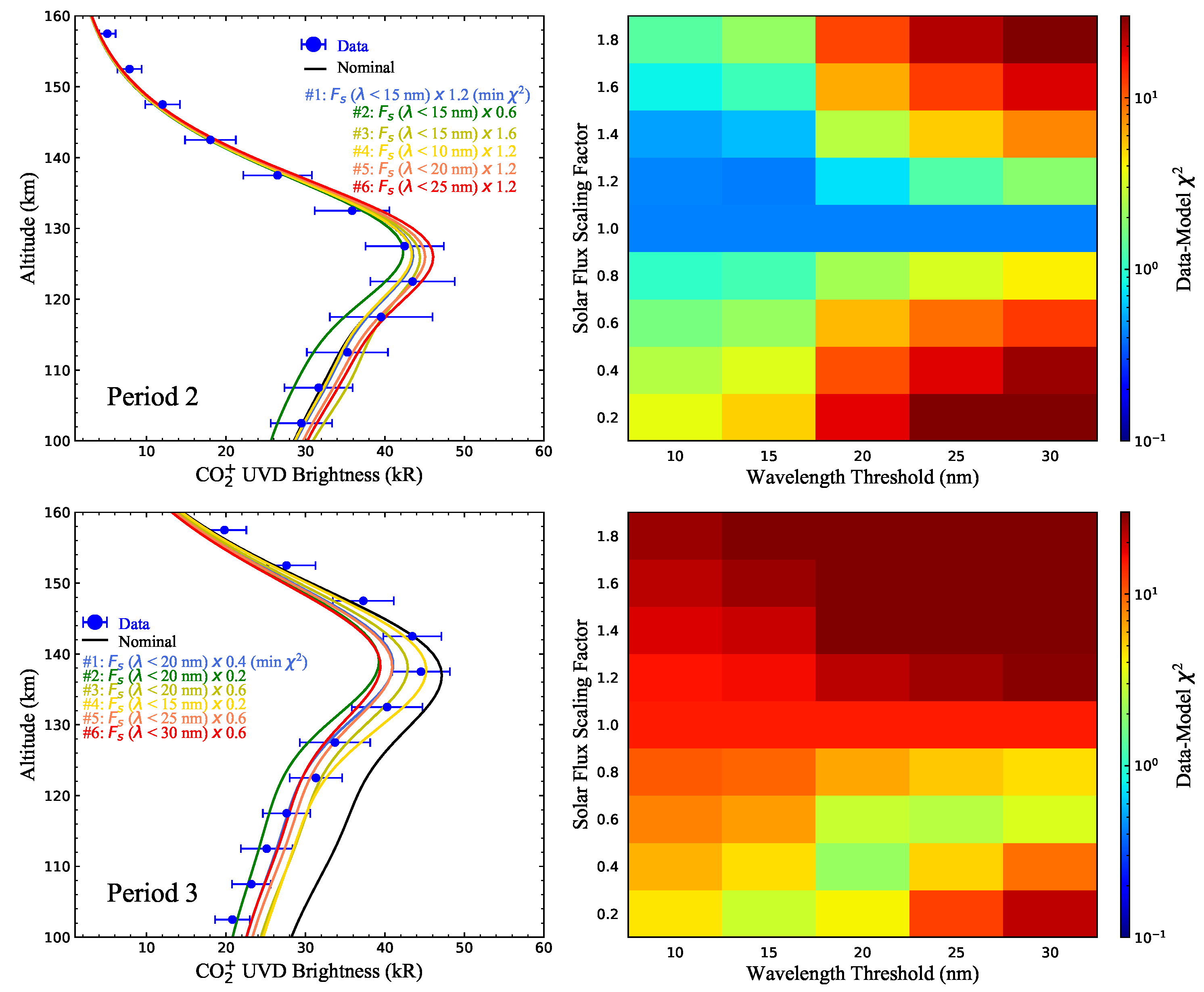
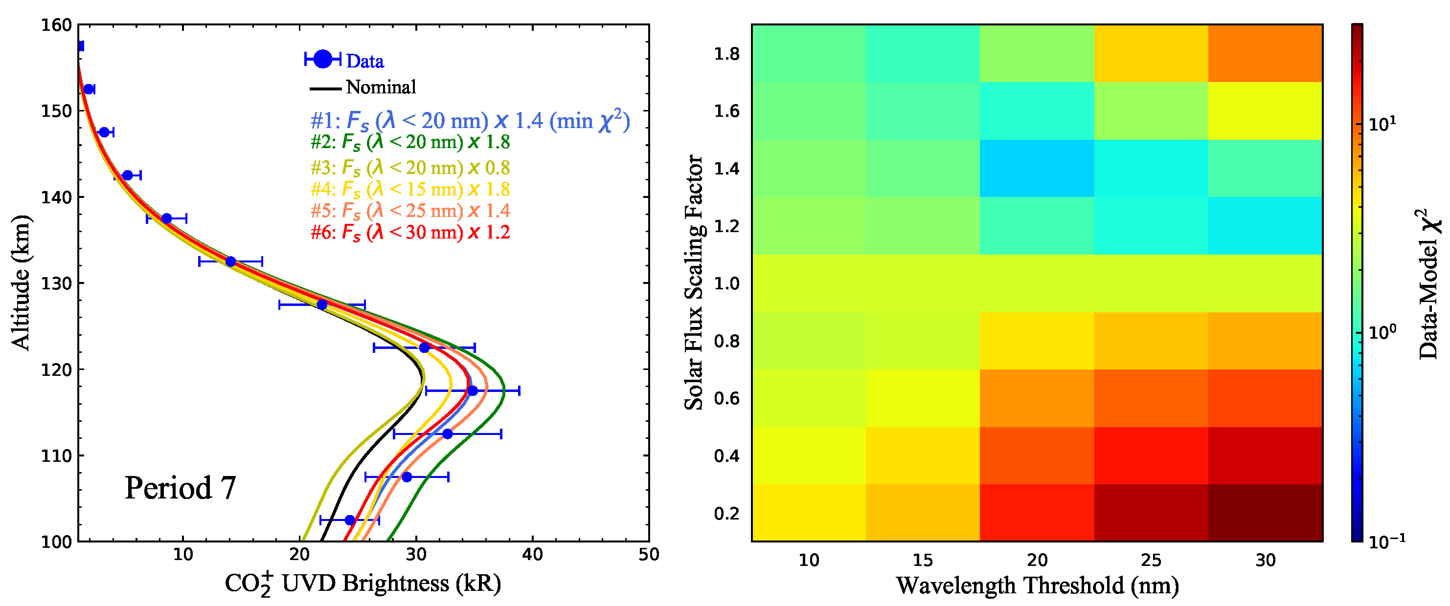
5. Sources of the Data–Model Discrepancy
5.1. Background Atmosphere
5.2. Incident Solar Spectrum
6. Conclusions
Author Contributions
Funding
Institutional Review Board Statement
Informed Consent Statement
Data Availability Statement
Conflicts of Interest
References
- Barth, C.A.; Fastie, W.G.; Hord, C.W.; Pearce, J.B.; Kelly, K.K.; Stewart, A.I.; Thomas, G.E.; Anderson, G.P.; Raper, O.F. Marine 6: Ultraviolet Spectrum of Mars Upper Atmosphere. Science 1969, 165, 1004–1005. [Google Scholar] [CrossRef] [PubMed]
- Barth, C.A.; Hord, C.W.; Pearce, J.B.; Kelly, K.K.; Anderson, G.P.; Stewart, A.I. Mariner 6 and 7 Ultraviolet Spectrometer Experiment: Upper atmosphere data. J. Geophys. Res. 1971, 76, 2213. [Google Scholar] [CrossRef] [Green Version]
- Stewart, A.I. Mariner 6 and 7 Ultraviolet Spectrometer Experiment: Implications of CO, CO and O Airglow. J. Geophys. Res. 1972, 77, 54. [Google Scholar] [CrossRef]
- Stewart, A.I.; Barth, C.A.; Hord, C.W.; Lane, A.L. Mariner 9 Ultraviolet Spectrometer Experiment: Structure of Mars’s Upper Atmosphere (A 5. 3). Icarus 1972, 17, 469–474. [Google Scholar] [CrossRef]
- Leblanc, F.; Chaufray, J.Y.; Lilensten, J.; Witasse, O.; Bertaux, J.L. Martian dayglow as seen by the SPICAM UV spectrograph on Mars Express. J. Geophys. Res. Planets 2006, 111, E09S11. [Google Scholar] [CrossRef]
- Cox, C.; Gérard, J.C.; Hubert, B.; Bertaux, J.L.; Bougher, S.W. Mars ultraviolet dayglow variability: SPICAM observations and comparison with airglow model. J. Geophys. Res. Planets 2010, 115, E04010. [Google Scholar] [CrossRef] [Green Version]
- Stiepen, A.; Gérard, J.C.; Bougher, S.; Montmessin, F.; Hubert, B.; Bertaux, J.L. Mars thermospheric scale height: CO Cameron and CO dayglow observations from Mars Express. Icarus 2015, 245, 295–305. [Google Scholar] [CrossRef]
- Montmessin, F.; Korablev, O.; Lefèvre, F.; Bertaux, J.L.; Fedorova, A.; Trokhimovskiy, A.; Chaufray, J.Y.; Lacombe, G.; Reberac, A.; Maltagliati, L.; et al. SPICAM on Mars Express: A 10 year in-depth survey of the Martian atmosphere. Icarus 2017, 297, 195–216. [Google Scholar] [CrossRef]
- Jain, S.K.; Stewart, A.I.F.; Schneider, N.M.; Deighan, J.; Stiepen, A.; Evans, J.S.; Stevens, M.H.; Chaffin, M.S.; Crismani, M.; McClintock, W.E.; et al. The structure and variability of Mars upper atmosphere as seen in MAVEN/IUVS dayglow observations. Geophys. Res. Lett. 2015, 42, 9023–9030. [Google Scholar] [CrossRef] [Green Version]
- Jain, S.K.; Deighan, J.; Schneider, N.M.; Stewart, A.I.F.; Evans, J.S.; Thiemann, E.M.B.; Chaffin, M.S.; Crismani, M.; Stevens, M.H.; Elrod, M.K.; et al. Martian Thermospheric Response to an X8.2 Solar Flare on 10 September 2017 as Seen by MAVEN/IUVS. Geophys. Res. Lett. 2018, 45, 7312–7319. [Google Scholar] [CrossRef] [Green Version]
- Gérard, J.C.; Gkouvelis, L.; Ritter, B.; Hubert, B.; Jain, S.K.; Schneider, N.M. MAVEN-IUVS Observations of the CO UV Doublet and CO Cameron Bands in the Martian Thermosphere: Aeronomy, Seasonal, and Latitudinal Distribution. J. Geophys. Res. Space Phys. 2019, 124, 5816–5827. [Google Scholar] [CrossRef]
- Li, Z.; Cui, J.; Li, J.; Wu, X.; Zhong, J.; Jian, F. Solar control of CO ultraviolet doublet emission on Mars. Earth Planet. Phys. 2020, 4, 543–549. [Google Scholar] [CrossRef]
- Qin, J. Solar Cycle, Seasonal, and Dust-storm-driven Variations of the Mars Upper Atmospheric State and H Escape Rate Derived from the Lyα Emission Observed by NASA’s MAVEN Mission. Astrophys. J. 2021, 912, 77. [Google Scholar] [CrossRef]
- Fox, J.L.; Dalgarno, A. Ionization, luminosity, and heating of the upper atmosphere of Mars. J. Geophys. Res. 1979, 84, 7315–7333. [Google Scholar] [CrossRef] [Green Version]
- Shematovich, V.I.; Bisikalo, D.V.; Gérard, J.C.; Cox, C.; Bougher, S.W.; Leblanc, F. Monte Carlo model of electron transport for the calculation of Mars dayglow emissions. J. Geophys. Res. Planets 2008, 113, E02011. [Google Scholar] [CrossRef] [Green Version]
- Simon, C.; Witasse, O.; Leblanc, F.; Gronoff, G.; Bertaux, J.L. Dayglow on Mars: Kinetic modelling with SPICAM UV limb data. Planet. Space Sci. 2009, 57, 1008–1021. [Google Scholar] [CrossRef]
- Jain, S.K.; Bhardwaj, A. Impact of solar EUV flux on CO Cameron band and CO UV doublet emissions in the dayglow of Mars. Planet. Space Sci. 2012, 63, 110–122. [Google Scholar] [CrossRef] [Green Version]
- González-Galindo, F.; Chaufray, J.Y.; Forget, F.; García-Comas, M.; Montmessin, F.; Jain, S.K.; Stiepen, A. UV Dayglow Variability on Mars: Simulation With a Global Climate Model and Comparison With SPICAM/MEx Data. J. Geophys. Res. Planets 2018, 123, 1934–1952. [Google Scholar] [CrossRef]
- Nier, A.O.; McElroy, M.B. Structure of the Neutral Upper Atmosphere of Mars: Results from Viking 1 and Viking 2. Science 1976, 194, 1298–1300. [Google Scholar] [CrossRef]
- Bougher, S.W.; Murphy, J.R.; Bell, J.M.; Zurek, R.W. Prediction of the structure of the martian upper atmosphere for the Mars Reconnaissance Orbiter (MRO) mission. Int. J. Mars Sci. Explor. 2006, 2, 10–20. [Google Scholar] [CrossRef]
- Bougher, S.W.; McDunn, T.M.; Zoldak, K.A.; Forbes, J.M. Solar cycle variability of Mars dayside exospheric temperatures: Model evaluation of underlying thermal balances. Geophys. Res. Lett. 2009, 36, L05201. [Google Scholar] [CrossRef] [Green Version]
- Forget, F.; Montmessin, F.; Bertaux, J.L.; González-Galindo, F.; Lebonnois, S.; Quémerais, E.; Reberac, A.; Dimarellis, E.; López-Valverde, M.A. Density and temperatures of the upper Martian atmosphere measured by stellar occultations with Mars Express SPICAM. J. Geophys. Res. Planets 2009, 114, E01004. [Google Scholar] [CrossRef] [Green Version]
- Liemohn, M.W.; Ma, Y.; Kozyra, J.U.; Nagy, A.F.; Frahm, R.A.; Winningham, J.D.; Sharber, J.R.; Barabash, S.V.; Lundin, R.N.; Team, T. MHD and kinetic modeling analysis of high-altitude photoelectron observations at Mars. In AGU Spring Meeting Abstracts; American Geophysical Union: New Orleans, LA, USA, 2005; Volume 2005, p. SA32A-05. [Google Scholar]
- Xu, S.; Liemohn, M.W.; Peterson, W.K.; Fontenla, J.; Chamberlin, P. Comparison of different solar irradiance models for the superthermal electron transport model for Mars. Planet. Space Sci. 2015, 119, 62–68. [Google Scholar] [CrossRef] [Green Version]
- Peterson, W.K.; Thiemann, E.M.B.; Eparvier, F.G.; Andersson, L.; Fowler, C.M.; Larson, D.; Mitchell, D.; Mazelle, C.; Fontenla, J.; Evans, J.S.; et al. Photoelectrons and solar ionizing radiation at Mars: Predictions versus MAVEN observations. J. Geophys. Res. Space Phys. 2016, 121, 8859–8870. [Google Scholar] [CrossRef]
- Jakosky, B.M.; Lin, R.P.; Grebowsky, J.M.; Luhmann, J.G.; Mitchell, D.F.; Beutelschies, G.; Priser, T.; Acuna, M.; Andersson, L.; Baird, D.; et al. The Mars Atmosphere and Volatile Evolution (MAVEN) Mission. Space Sci. Rev. 2015, 195, 3–48. [Google Scholar] [CrossRef]
- McClintock, W.E.; Schneider, N.M.; Holsclaw, G.M.; Clarke, J.T.; Hoskins, A.C.; Stewart, I.; Montmessin, F.; Yelle, R.V.; Deighan, J. The Imaging Ultraviolet Spectrograph (IUVS) for the MAVEN Mission. Space Sci. Rev. 2015, 195, 75–124. [Google Scholar] [CrossRef]
- Mahaffy, P.R.; Benna, M.; King, T.; Harpold, D.N.; Arvey, R.; Barciniak, M.; Bendt, M.; Carrigan, D.; Errigo, T.; Holmes, V.; et al. The Neutral Gas and Ion Mass Spectrometer on the Mars Atmosphere and Volatile Evolution Mission. Space Sci. Rev. 2015, 195, 49–73. [Google Scholar] [CrossRef] [Green Version]
- Mitchell, D.L.; Mazelle, C.; Sauvaud, J.A.; Thocaven, J.J.; Rouzaud, J.; Fedorov, A.; Rouger, P.; Toublanc, D.; Taylor, E.; Gordon, D.; et al. The MAVEN Solar Wind Electron Analyzer. Space Sci. Rev. 2016, 200, 495–528. [Google Scholar] [CrossRef]
- Eparvier, F.G.; Chamberlin, P.C.; Woods, T.N.; Thiemann, E.M.B. The Solar Extreme Ultraviolet Monitor for MAVEN. Space Sci. Rev. 2015, 195, 293–301. [Google Scholar] [CrossRef]
- Gronoff, G.; Simon Wedlund, C.; Mertens, C.J.; Barthélemy, M.; Lillis, R.J.; Witasse, O. Computing uncertainties in ionosphere-airglow models: II. The Martian airglow. J. Geophys. Res. Space Phys. 2012, 117, A05309. [Google Scholar] [CrossRef] [Green Version]
- Evans, J.S.; Stevens, M.H.; Lumpe, J.D.; Schneider, N.M.; Stewart, A.I.F.; Deighan, J.; Jain, S.K.; Chaffin, M.S.; Crismani, M.; Stiepen, A.; et al. Retrieval of CO2 and N2 in the Martian thermosphere using dayglow observations by IUVS on MAVEN. Geophys. Res. Lett. 2015, 42, 9040–9049. [Google Scholar] [CrossRef] [Green Version]
- Wu, X.; Cui, J.; Niu, D.; Ren, Z.; Wei, Y. Compositional Variation of the Dayside Martian Ionosphere: Inference from Photochemical Equilibrium Computations. Astrophys. J. 2021, 923, 29. [Google Scholar] [CrossRef]
- Johnson, M.A.; Zare, R.N.; Rostas, J.; Leach, S. Resolution of the Ã/B∼ photoionization branching ratio paradox for the 12CO B∼(000) state. J. Chem. Phys. 1984, 80, 2407–2428. [Google Scholar] [CrossRef]
- Leach, S.; Stannard, P.R.; Gelbart, W.M. Interelectronic-state perturbation effects on photoelectron spectra and emission quantum yields. Mol. Phys. 1978, 36, 1119–1132. [Google Scholar] [CrossRef]
- Samson, J.A.R.; Gardner, J.L. Fluorescence excitation and photoelectron spectra of CO2 induced by vacuum ultraviolet radiation between 185 and 716 Angstroms. J. Geophys. Res. 1973, 78, 3663. [Google Scholar] [CrossRef]
- Padial, N.; Csanak, G.; McKoy, B.V.; Langhoff, P.W. Photoexcitation and ionization in carbon dioxide: Theoretical studies in the separated-channel static-exchange approximation. Phys. Rev. A Gen. Phys. 1981, 23, 218–235. [Google Scholar] [CrossRef] [Green Version]
- Avakyan, S.V.; Ii’In, R.N.; Lavrov, V.M.; Ogurtsov, G.N. Collision Processes and Excitation of UV Emission from Planetary Atmospheric Gases: A Handbook of Cross Sections; CRC Press: Boca Raton, FL, USA, 1998. [Google Scholar]
- Thiemann, E.M.B.; Chamberlin, P.C.; Eparvier, F.G.; Templeman, B.; Woods, T.N.; Bougher, S.W.; Jakosky, B.M. The MAVEN EUVM model of solar spectral irradiance variability at Mars: Algorithms and results. J. Geophys. Res. Space Phys. 2017, 122, 2748–2767. [Google Scholar] [CrossRef]
- Chamberlin, P.C.; Eparvier, F.G.; Knoer, V.; Leise, H.; Pankratz, A.; Snow, M.; Templeman, B.; Thiemann, E.M.B.; Woodraska, D.L.; Woods, T.N. The Flare Irradiance Spectral Model-Version 2 (FISM2). Space Weather 2020, 18, e02588. [Google Scholar] [CrossRef]
- Krasnopolsky, V.A. Mars’ upper atmosphere and ionosphere at low, medium, and high solar activities: Implications for evolution of water. J. Geophys. Res. Planets 2002, 107, 5128. [Google Scholar] [CrossRef]
- Slipski, M.; Jakosky, B.Â.M.; Benna, M.; Elrod, M.; Mahaffy, P.; Kass, D.; Stone, S.; Yelle, R. Variability of Martian Turbopause Altitudes. J. Geophys. Res. Planets 2018, 123, 2939–2957. [Google Scholar] [CrossRef]
- Wu, X.S.; Cui, J.; Yelle, R.V.; Cao, Y.T.; He, Z.G.; He, F.; Wei, Y. Photoelectrons as a Tracer of Planetary Atmospheric Composition: Application to CO on Mars. J. Geophys. Res. Planets 2020, 125, e06441. [Google Scholar] [CrossRef]
- Lillis, R.J.; Deighan, J.; Fox, J.L.; Bougher, S.W.; Lee, Y.; Combi, M.R.; Cravens, T.E.; Rahmati, A.; Mahaffy, P.R.; Benna, M.; et al. Photochemical escape of oxygen from Mars: First results from MAVEN in situ data. J. Geophys. Res. Space Phys. 2017, 122, 3815–3836. [Google Scholar] [CrossRef]
- Chaufray, J.Y.; Deighan, J.; Chaffin, M.S.; Schneider, N.M.; McClintock, W.E.; Stewart, A.I.F.; Jain, S.K.; Crismani, M.; Stiepen, A.; Holsclaw, G.M.; et al. Study of the Martian cold oxygen corona from the O I 130.4 nm by IUVS/MAVEN. Geophys. Res. Lett. 2015, 42, 9031–9039. [Google Scholar] [CrossRef] [Green Version]
- Fox, J.L.; Johnson, A.S.; Ard, S.G.; Shuman, N.S.; Viggiano, A.A. Photochemical determination of O densities in the Martian thermosphere: Effect of a revised rate coefficient. Geophys. Res. Lett. 2017, 44, 8099–8106. [Google Scholar] [CrossRef]
- Mukundan, V.; Thampi, S.V.; Bhardwaj, A.; Krishnaprasad, C. The dayside ionosphere of Mars: Comparing a one-dimensional photochemical model with MAVEN Deep Dip campaign observations. Icarus 2020, 337, 113502. [Google Scholar] [CrossRef]
- Green, A.E.S.; Jackman, C.H.; Garvey, R.H. Electron impact on atmospheric gases, 2. Yield spectra. J. Geophys. Res. 1977, 82, 5104. [Google Scholar] [CrossRef]
- Bhardwaj, A.; Jain, S.K. Monte Carlo model of electron energy degradation in a CO2 atmosphere. J. Geophys. Res. Space Phys. 2009, 114, A11309. [Google Scholar] [CrossRef] [Green Version]
- Stevens, M.H.; Evans, J.S.; Schneider, N.M.; Stewart, A.I.F.; Deighan, J.; Jain, S.K.; Crismani, M.; Stiepen, A.; Chaffin, M.S.; McClintock, W.E.; et al. New observations of molecular nitrogen in the Martian upper atmosphere by IUVS on MAVEN. Geophys. Res. Lett. 2015, 42, 9050–9056. [Google Scholar] [CrossRef] [Green Version]
- Gkouvelis, L.; Gérard, J.C.; Ritter, B.; Hubert, B.; Schneider, N.M.; Jain, S.K. The O(1S) 297.2-nm Dayglow Emission: A Tracer of CO2 Density Variations in the Martian Lower Thermosphere. J. Geophys. Res. Planets 2018, 123, 3119–3132. [Google Scholar] [CrossRef]
- Cui, J.; Wu, X.S.; Xu, S.S.; Wang, X.D.; Wellbrock, A.; Nordheim, T.A.; Cao, Y.T.; Wang, W.R.; Sun, W.Q.; Wu, S.Q.; et al. Ionization Efficiency in the Dayside Martian Upper Atmosphere. Astrophys. J. Lett. 2018, 857, L18. [Google Scholar] [CrossRef]
- Lillis, R.J.; Xu, S.; Mitchell, D.; Thiemann, E.; Eparvier, F.; Benna, M.; Elrod, M. Ionization Efficiency in the Dayside Ionosphere of Mars: Structure and Variability. J. Geophys. Res. Planets 2021, 126, e06923. [Google Scholar] [CrossRef]
- Fox, J.L.; Galand, M.I.; Johnson, R.E. Energy Deposition in Planetary Atmospheres by Charged Particles and Solar Photons. Space Sci. Rev. 2008, 139, 3–62. [Google Scholar] [CrossRef]
- Wang, J.S.; Nielsen, E. Behavior of the Martian dayside electron density peak during global dust storms. Planet. Space Sci. 2003, 51, 329–338. [Google Scholar] [CrossRef]
- Withers, P.; Pratt, R. An observational study of the response of the upper atmosphere of Mars to lower atmospheric dust storms. Icarus 2013, 225, 378–389. [Google Scholar] [CrossRef] [Green Version]
- Liu, G.; England, S.L.; Lillis, R.J.; Withers, P.; Mahaffy, P.R.; Rowland, D.E.; Elrod, M.; Benna, M.; Kass, D.M.; Janches, D.; et al. Thermospheric Expansion Associated With Dust Increase in the Lower Atmosphere on Mars Observed by MAVEN/NGIMS. Geophys. Res. Lett. 2018, 45, 2901–2910. [Google Scholar] [CrossRef]
- Fox, J.L.; Benna, M.; McFadden, J.P.; Jakosky, B.M.; Maven Ngims Team. Rate coefficients for the reactions of CO with O: Lessons from MAVEN at Mars. Icarus 2021, 358, 114186. [Google Scholar] [CrossRef]
- Mahaffy, P.R.; Benna, M.; Elrod, M.; Yelle, R.V.; Bougher, S.W.; Stone, S.W.; Jakosky, B.M. Structure and composition of the neutral upper atmosphere of Mars from the MAVEN NGIMS investigation. Geophys. Res. Lett. 2015, 42, 8951–8957. [Google Scholar] [CrossRef] [Green Version]
- Tobiska, W.K.; Woods, T.; Eparvier, F.; Viereck, R.; Floyd, L.; Bouwer, D.; Rottman, G.; White, O.R. The SOLAR2000 empirical solar irradiance model and forecast tool. J. Atmos. Sol.-Terr. Phys. 2000, 62, 1233–1250. [Google Scholar] [CrossRef]
- Richards, P.G.; Fennelly, J.A.; Torr, D.G. EUVAC: A solar EUV flux model for aeronomic calculations. J. Geophys. Res. 1994, 99, 8981–8992. [Google Scholar] [CrossRef]
- Jain, S.K.; Bhardwaj, A. Model calculation of N2 Vegard-Kaplan band emissions in Martian dayglow. J. Geophys. Res. Planets 2011, 116, E07005. [Google Scholar] [CrossRef] [Green Version]
- Peterson, W.K.; Woods, T.N.; Fontenla, J.M.; Richards, P.G.; Chamberlin, P.C.; Solomon, S.C.; Tobiska, W.K.; Warren, H.P. Solar EUV and XUV energy input to thermosphere on solar rotation time scales derived from photoelectron observations. J. Geophys. Res. Space Phys. 2012, 117, A05320. [Google Scholar] [CrossRef] [Green Version]


| Period | Date | Ls | SZA | Latitude | Solar Flux 1 |
|---|---|---|---|---|---|
| (erg s−1 cm−2) | |||||
| 1 | 11 October 2015–13 November 2015 | 64° | 55–60° (57°) | 40–17°S (29°S) | 0.98 |
| 2 | 6 April 2016–12 May 2016 | 140° | 52–60° (55°) | 55–74° (66°) | 0.95 |
| 3 | 15 October 2016–29 November 2016 | 259° | 46–60° (51°) | 74–57°S (68°S) | 1.04 |
| 4 | 4 April 2017–17 April 2017 | 346° | 45–60° (52°) | 6–15° (11°) | 0.9 |
| 5 | 1 June 2017–16 June 2017 | 18° | 45–60° (52°) | 47–57° (52°) | 0.78 |
| 6 | 19 September 2017–2 October 2017 | 69° | 45–60° (52°) | 32–41° (36°) | 0.68 |
| 7 | 27 November 2017–8 December 2017 | 97° | 45–60° (52°) | 19–11°S (15°S) | 0.68 |
| 8 | 22 April 2018–6 June 2018 | 175° | 45–60° (50°) | 53–20°S (37°S) | 0.86 |
| 9 | 4 October 2019–15 October 2019 | 91° | 45–60° (52°) | 70–75° (73°) | 0.63 |
| 10 | 28 January 2020–19 February 2020 | 148° | 56–60° (57°) | 49–26°S (38°S) | 0.76 |
| IUVS | Model (Original 1) | Model (Adjusted 2) | ||||
|---|---|---|---|---|---|---|
| Period | Brightness | Altitude | Brightness | Altitude | Brightness | Altitude |
| kR | km | kR | km | kR | km | |
| 1 | 42.7 | 117.5 | 41 | 117 | 42.5 | 118 |
| 2 | 43.8 | 124.1 | 40 | 126 | 43.5 | 126 |
| 3 | 45.0 | 139.0 | 44 | 137 | 45.2 | 138 |
| 4 | 44.3 | 125.0 | 41 | 126 | 42.8 | 126 |
| 5 | 32.8 | 118.5 | 31 | 121 | 31.7 | 121 |
| 6 | 26.5 | 121.4 | 26 | 121 | 26.2 | 122 |
| 7 | 34.9 | 117.0 | 28 | 119 | 34.7 | 118 |
| 8 | 35.7 | 122.3 | 37 | 121 | 34.6 | 122 |
| 9 | 30.9 | 122.4 | 27 | 122 | 30.0 | 122 |
| 10 | 30.9 | 121.2 | 34 | 119 | 30.2 | 120 |
Publisher’s Note: MDPI stays neutral with regard to jurisdictional claims in published maps and institutional affiliations. |
© 2022 by the authors. Licensee MDPI, Basel, Switzerland. This article is an open access article distributed under the terms and conditions of the Creative Commons Attribution (CC BY) license (https://creativecommons.org/licenses/by/4.0/).
Share and Cite
Li, Z.; Niu, D.; Gu, H.; Wu, X.; Huang, Y.; Zhong, J.; Cui, J.
Modeling the CO
Li Z, Niu D, Gu H, Wu X, Huang Y, Zhong J, Cui J.
Modeling the CO
Li, Zichuan, Dandan Niu, Hao Gu, Xiaoshu Wu, Yingying Huang, Jiahao Zhong, and Jun Cui.
2022. "Modeling the CO