
From Forest Dynamics to Wetland Siltation in Mountainous Landscapes: A RS-Based Framework for Enhancing Erosion Control

 ,
,
Abstract
:1. Introduction
2. Objectives
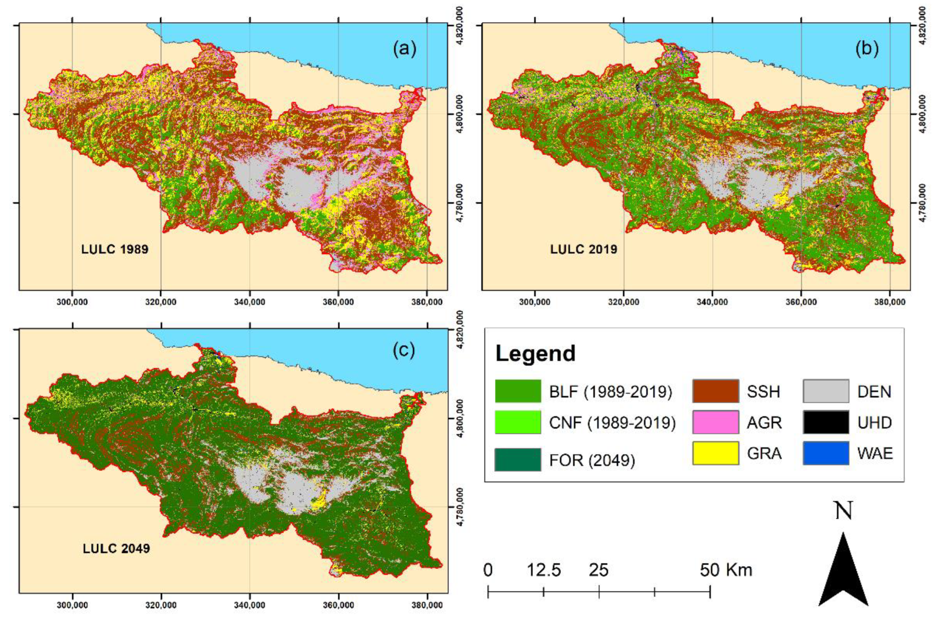
- Mapping LULC dynamics from 1989 to 2019 by coupling Landsat and Sentinel 2 imagery.
- Modelling forest distribution in a future scenario for 2049 based on a reliable maximum forest cover increment defined for the study area.
- Mapping current wetlands distribution supported by extensive fieldwork and photo-interpretation.
- Modelling landscape processes related to the production, transport and deposition of sediment.
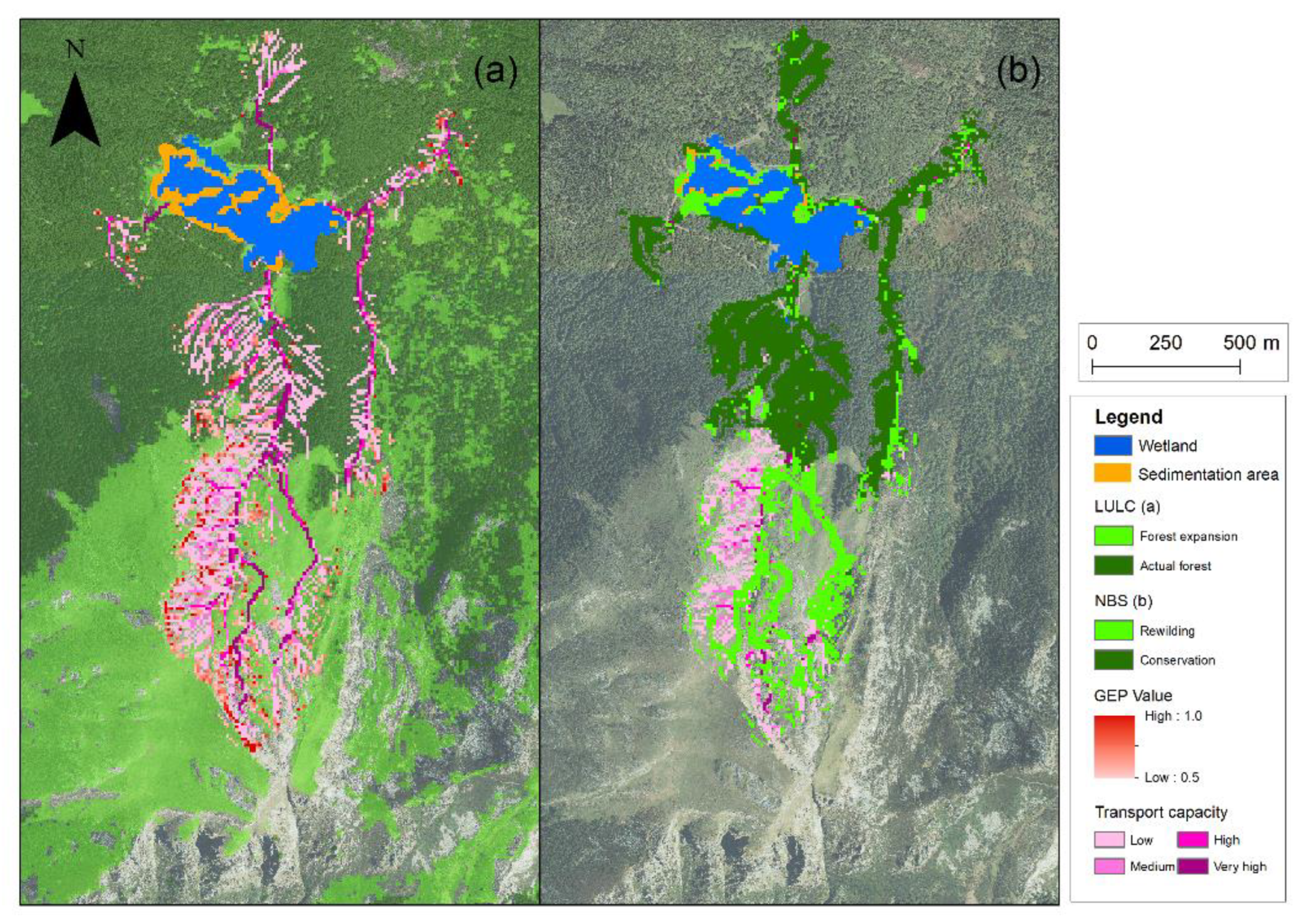
- Application of multi-criteria analyses to identify potential areas for the implementation of NBS (i.e., forest restoration and conservation) to reduce erosion effects on wetland ecosystems.
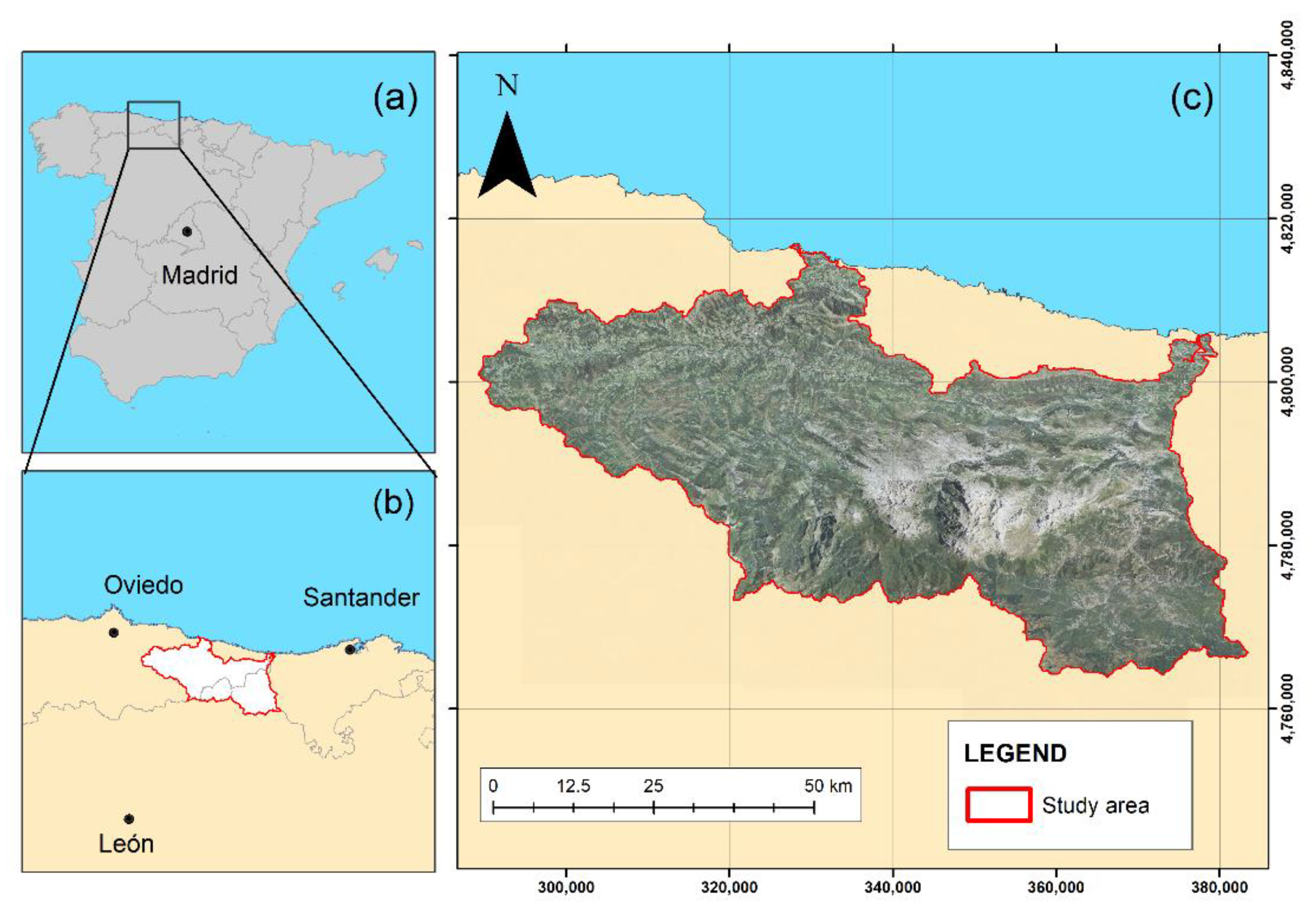
3. Study Area
4. Materials and Methods
4.1. In Situ Data across Environmental Gradients
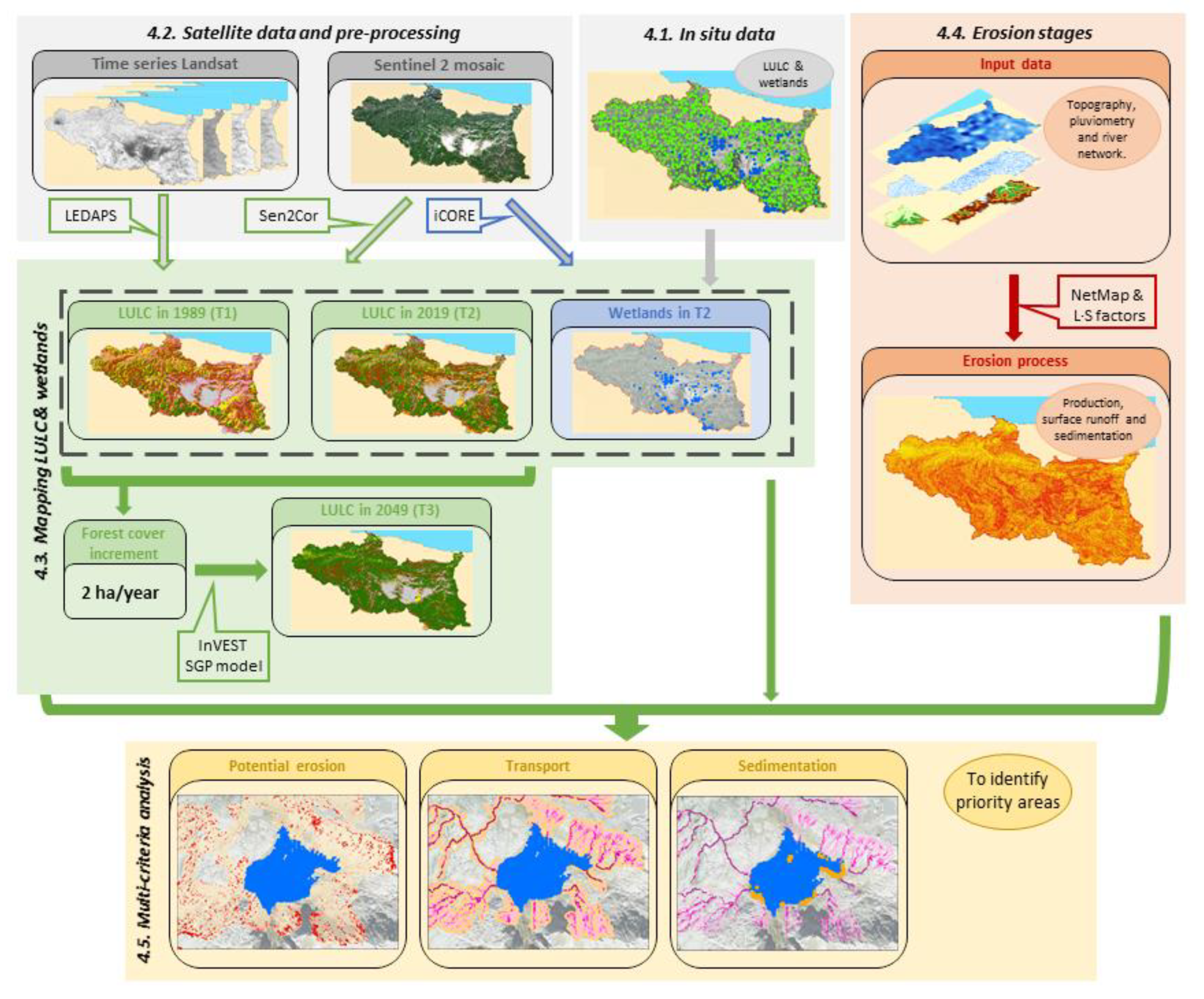
4.2. Satellite Data and Pre-Processing
4.3. Mapping LULC Trends and Wetlands Distribution
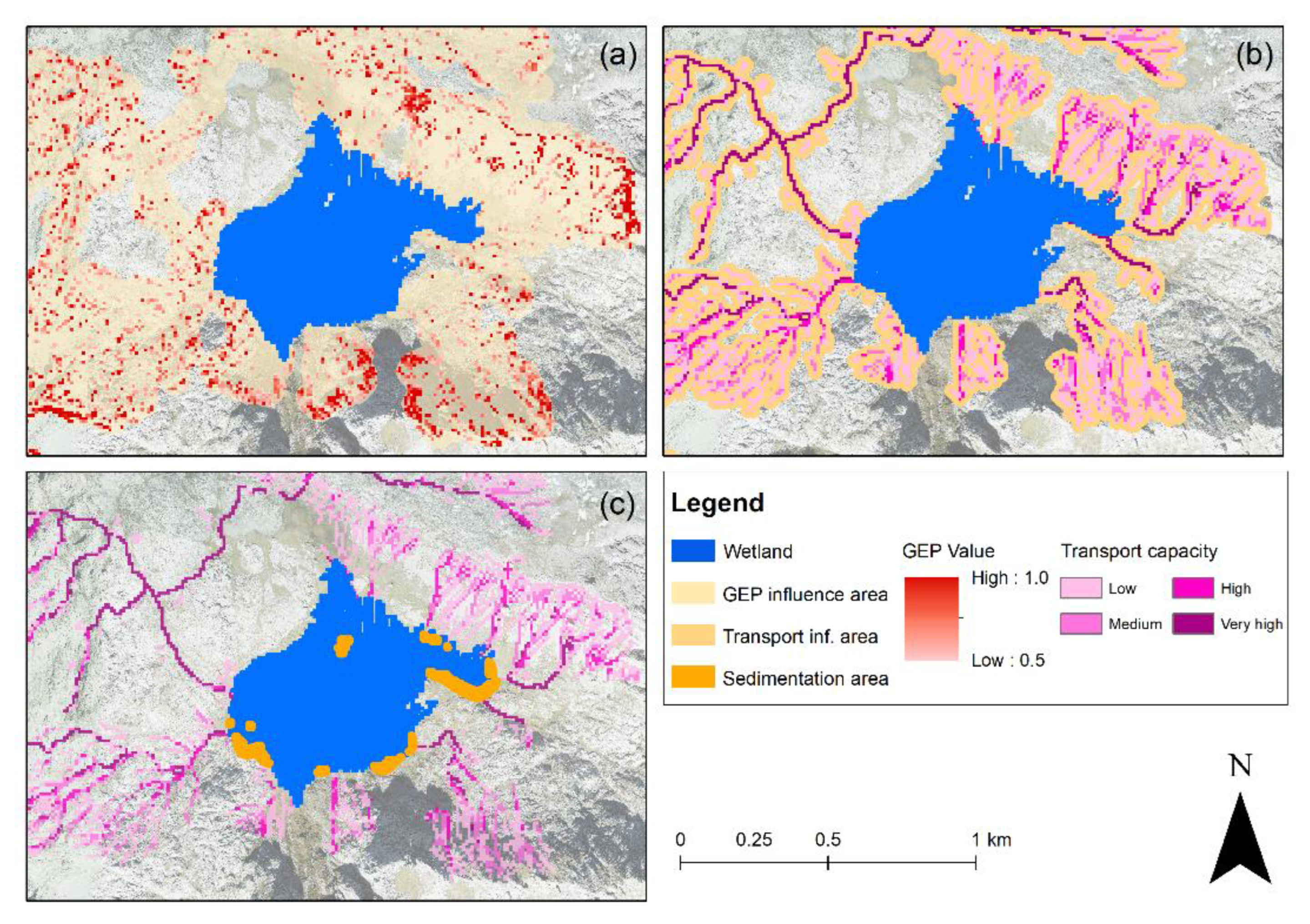
4.4. Potential Erosion, Surface Runoff and Deposition Areas
4.5. Multi-Criteria Analysis: From Forest Dynamics to Wetland Siltation
5. Results
6. Discussion
6.1. Landscape Modelling Approach
6.2. Implications for Landscape Management
7. Conclusions
Author Contributions
Funding
Institutional Review Board Statement
Informed Consent Statement
Data Availability Statement
Acknowledgments
Conflicts of Interest
References
- Biswas, A.K. Integrated water resources management: A reassessment: A water forum contribution. Water Int. 2004, 29, 248–256. [Google Scholar] [CrossRef]
- Flores Díaz, A.C.; Mokondoko Delgadillo, P.; González Mora, I.; Machorro Reyes, J.; Ríos Patrón, E. Servicios Ecosistémicos: Fundamentos desde el Manejo de Cuencas. Cuadernos de Divulgación Ambiental. 2018. Available online: https://agua.org.mx/wp-content/uploads/2018/05/Servicios-ecosistémicos-fundamentos-desde-el-manejo-de-cuencas.pdf (accessed on 11 January 2022).
- Sadoff, C.; Muller, M. Water Management, Water Security and Climate Change Adaptation: Early Impacts and Essential Responses; Global Water Partnership Stockholm: Stockholm, Sweden, 2009. [Google Scholar]
- Pérez-Silos, I.; Álvarez-Martínez, J.M.; Barquín, J. Large-scale afforestation for ecosystem service provisioning: Learning from the past to improve the future. Landsc. Ecol. 2021, 36, 3329–3343. [Google Scholar] [CrossRef]
- Troy, A.; Wilson, M.A. Mapping Ecosystem Services: Practical challenges and opportunities in linking GIS and value transfer. Ecol. Econ. 2006, 60, 435–449. [Google Scholar] [CrossRef]
- Duarte, R.; Pinilla, V.; Serrano, A. Globalization and natural resources: The expansion of the Spanish agrifood trade and its impact on water consumption, 1965–2010. Reg. Environ. Chang. 2016, 16, 259–272. [Google Scholar] [CrossRef] [Green Version]
- Thornton, P.; Herrero, M. The Inter-Linkages between Rapid Growth in Livestock Production, Climate Change, and the Impacts on Water Resources, Land Use, and Deforestation. 2010. Available online: https://ssrn.com/abstract=1536991 (accessed on 11 January 2022).
- Benayas, J.M.R.; Bullock, J.M. Restoration of biodiversity and Ecosystem Services on agricultural land. Ecosystems 2012, 15, 883–899. [Google Scholar] [CrossRef]
- Power, A.G. Ecosystem Services and agriculture: Tradeoffs and synergies. Philos. Trans. R. Soc. B Biol. Sci. 2010, 365, 2959–2971. [Google Scholar] [CrossRef]
- Hein, L.; Van Koppen, K.; De Groot, R.S.; Van Ierland, E.C. Spatial scales, stakeholders and the valuation of Ecosystem Services. Ecol. Econ. 2006, 57, 209–228. [Google Scholar] [CrossRef]
- Reid, W.V.; Mooney, H.A.; Capistrano, D.; Carpenter, S.R.; Chopra, K.; Cropper, A.; Dasgupta, P.; Hassan, R.; Leemans, R.; May, R.M. Nature: The many benefits of Ecosystem Services. Nature 2006, 443, 749. [Google Scholar] [CrossRef]
- Chiabai, A.; Quiroga, S.; Martinez-Juarez, P.; Higgins, S.; Taylor, T. The nexus between climate change, Ecosystem Services and human health: Towards a conceptual framework. Sci. Total Environ. 2018, 635, 1191–1204. [Google Scholar] [CrossRef]
- Daily, G. Introduction: What are Ecosystem Services. In Nature’s Services: Societal Dependence on Natural Ecosystems; Daily, Gretchen: Washington, DC, USA, 1997; Volume 1. [Google Scholar]
- De Groot, R.S.; Alkemade, R.; Braat, L.; Hein, L.; Willemen, L. Challenges in integrating the concept of Ecosystem Services and values in landscape planning, management and decision making. Ecol. Complex. 2010, 7, 260–272. [Google Scholar] [CrossRef]
- Haines-Young, R.; Potschin, M. The links between biodiversity, Ecosystem Services and human well-being. Ecosyst. Ecol. A New Synth. 2010, 1, 110–139. [Google Scholar]
- Heywood, V.; Stuart, S. Species extinctions in tropical forests. Trop. Deforestation Species Extinction 1992, 5, 91–117. [Google Scholar]
- Seidl, R.; Schelhaas, M.-J.; Rammer, W.; Verkerk, P.J. Increasing forest disturbances in Europe and their impact on carbon storage. Nat. Clim. Chang. 2014, 4, 806–810. [Google Scholar] [CrossRef] [PubMed] [Green Version]
- McIntyre, S.; Hobbs, R. A framework for conceptualizing human effects on landscapes and its relevance to management and research models. Conserv. Biol. 1999, 13, 1282–1292. [Google Scholar] [CrossRef]
- Primack, R.B.; Ros, J. Introducción a la Biología de la Conservación; Grupo Planeta (GBS): Madrid, Spain, 2002. [Google Scholar]
- Duraiappah, A.K. Poverty and environmental degradation: A review and analysis of the nexus. World Dev. 1998, 26, 2169–2179. [Google Scholar] [CrossRef]
- Freedman, B. Environmental Ecology: The Ecological Effects of Pollution, Disturbance, and Other Stresses; Elsevier: Amsterdam, The Netherlands, 1995. [Google Scholar]
- Karr, J.R.; Dudley, D.R. Ecological perspective on water quality goals. Environ. Manag. 1981, 5, 55–68. [Google Scholar] [CrossRef]
- Daily, G. What are Ecosystem Services. Glob. Environ. Chall. Twenty-First Century Resour. Consum. Sustain. Solut. 2003, 1, 227–231. [Google Scholar]
- De Groot, R.S.; Wilson, M.A.; Boumans, R.M. A typology for the classification, description and valuation of ecosystem functions, goods and services. Ecol. Econ. 2002, 41, 393–408. [Google Scholar] [CrossRef] [Green Version]
- Council, N.R. Restoration of Aquatic Ecosystems: Science, Technology, and Public Policy; National Academies Press: Cambridge, MA, USA, 1992. [Google Scholar]
- Houlahan, J.E.; Keddy, P.A.; Makkay, K.; Findlay, C.S. The effects of adjacent land use on wetland species richness and community composition. Wetlands 2006, 26, 79–96. [Google Scholar] [CrossRef]
- Winter, T.C. The vulnerability of wetlands to climate change: A hydrologic landscape perspective 1. JAWRA J. Am. Water Resour. Assoc. 2000, 36, 305–311. [Google Scholar] [CrossRef]
- Detenbeck, N.E.; Taylor, D.L.; Lima, A.; Hagley, C. Temporal and spatial variability in water quality of wetlands in the Minneapolis/St. Paul, MN metropolitan area: Implications for monitoring strategies and designs. Environ. Monit. Assess. 1996, 40, 11–40. [Google Scholar] [CrossRef] [PubMed]
- Skagen, S.K.; Melcher, C.P.; Haukos, D.A. Reducing sedimentation of depressional wetlands in agricultural landscapes. Wetlands 2008, 28, 594–604. [Google Scholar] [CrossRef]
- Watson, J.E.; Evans, T.; Venter, O.; Williams, B.; Tulloch, A.; Stewart, C.; Thompson, I.; Ray, J.C.; Murray, K.; Salazar, A. The exceptional value of intact forest ecosystems. Nat. Ecol. Evol. 2018, 2, 599–610. [Google Scholar] [CrossRef] [PubMed]
- Gerten, D.; Schaphoff, S.; Haberlandt, U.; Lucht, W.; Sitch, S. Terrestrial vegetation and water balance—Hydrological evaluation of a dynamic global vegetation model. J. Hydrol. 2004, 286, 249–270. [Google Scholar] [CrossRef]
- Neary, D.G.; Ice, G.G.; Jackson, C.R. Linkages between forest soils and water quality and quantity. For. Ecol. Manag. 2009, 258, 2269–2281. [Google Scholar] [CrossRef]
- Acreman, M.; Holden, J. How wetlands affect floods. Wetlands 2013, 33, 773–786. [Google Scholar] [CrossRef] [Green Version]
- Alonso, J.L.; Pulgar, F.J.Á.; Pedreira, D. El relieve de la Cordillera Cantábrica. Enseñanza Cienc. Tierra 2007, 15, 151–163. [Google Scholar]
- Belmar, O.; Barquín, J.; Álvarez-Martínez, J.M.; Peñas, F.J.; Del Jesus, M. The role of forest maturity in extreme hydrological events. Ecohydrology 2018, 11, e1947. [Google Scholar] [CrossRef]
- Gillson, L.; Ladle, R.J.; Araújo, M.B. Baselines, patterns and process. In Conservation Biogeography; Wiley-Blackwell: Oxford, UK, 2011; Volume 1, pp. 31–44. [Google Scholar]
- Körner, C. Mountain biodiversity, its causes and function. AMBIO J. Hum. Environ. 2004, 33, 11–17. [Google Scholar] [CrossRef]
- Butler, J.R.; Marzano, M.; Pettorelli, N.; Durant, S.M.; du Toit, J.T.; Young, J.C. Decision-making for rewilding: An adaptive governance framework for social-ecological complexity. Front. Conserv. Sci. 2021, 2, 681545. [Google Scholar] [CrossRef]
- Perino, A.; Pereira, H.M.; Navarro, L.M.; Fernández, N.; Bullock, J.M.; Ceaușu, S.; Cortés-Avizanda, A.; van Klink, R.; Kuemmerle, T.; Lomba, A. Rewilding complex ecosystems. Science 2019, 364, eaav5570. [Google Scholar] [CrossRef] [PubMed] [Green Version]
- Borrelli, P.; Robinson, D.A.; Fleischer, L.R.; Lugato, E.; Ballabio, C.; Alewell, C.; Meusburger, K.; Modugno, S.; Schütt, B.; Ferro, V. An assessment of the global impact of 21st century land use change on soil erosion. Nat. Commun. 2017, 8, 2013. [Google Scholar] [CrossRef] [Green Version]
- Panagos, P.; Borrelli, P.; Poesen, J.; Ballabio, C.; Lugato, E.; Meusburger, K.; Montanarella, L.; Alewell, C. The new assessment of soil loss by water erosion in Europe. Environ. Sci. Policy 2015, 54, 438–447. [Google Scholar] [CrossRef]
- Maes, J.; Teller, A.; Erhard, M.; Liquete, C.; Braat, L.; Berry, P.; Egoh, B.; Puydarrieux, P.; Fiorina, C.; Santos, F. Mapping and Assessment of Ecosystems and their Services. Anal. Framew. Ecosyst. Assess. Under Action 2013, 5, 1–58. [Google Scholar]
- Hudson, N. Field Measurement of Soil Erosion and Runoff; Food & Agriculture Org.: Rome, Italy, 1993; Volume 68. [Google Scholar]
- Nearing, M.A.; Foster, G.R.; Lane, L.; Finkner, S. A process-based soil erosion model for USDA-Water Erosion Prediction Project technology. Trans. ASAE 1989, 32, 1587–1593. [Google Scholar] [CrossRef]
- Römkens, M.J.; Helming, K.; Prasad, S. Soil erosion under different rainfall intensities, surface roughness, and soil water regimes. Catena 2002, 46, 103–123. [Google Scholar] [CrossRef]
- Merritt, W.S.; Letcher, R.A.; Jakeman, A.J. A review of erosion and sediment transport models. Environ. Model. Softw. 2003, 18, 761–799. [Google Scholar] [CrossRef]
- McDowell, D.M. A general formula for estimation of the rate of transport of non-cohesive bed-load. J. Hydraul. Res. 1989, 27, 355–361. [Google Scholar] [CrossRef]
- Wohl, E. Legacy effects on sediments in river corridors. Earth-Sci. Rev. 2015, 147, 30–53. [Google Scholar] [CrossRef]
- Álvarez-Cobelas, M.; Sánchez-Carrillo, S.; Cirujano, S.; Angeler, D. A story of the wetland water quality deterioration: Salinization, pollution, eutrophication and siltation. Ecol. Threat. Semi-Arid Wetl. 2010, 2, 109–133. [Google Scholar]
- Johnston, C.A. Sediment and nutrient retention by freshwater wetlands: Effects on surface water quality. Crit. Rev. Environ. Control 1991, 21, 491–565. [Google Scholar] [CrossRef]
- Bilotta, G.S.; Brazier, R.E. Understanding the influence of suspended solids on water quality and aquatic biota. Water Res. 2008, 42, 2849–2861. [Google Scholar] [CrossRef] [PubMed]
- Davies-Colley, R.; Smith, D. Turbidity suspeni) ed sediment, and water clarity: A review 1. JAWRA J. Am. Water Resour. Assoc. 2001, 37, 1085–1101. [Google Scholar] [CrossRef]
- Wood, P.J.; Armitage, P.D. Biological effects of fine sediment in the lotic environment. Environ. Manag. 1997, 21, 203–217. [Google Scholar] [CrossRef]
- Fiskal, A.; Deng, L.; Michel, A.; Eickenbusch, P.; Han, X.; Lagostina, L.; Zhu, R.; Sander, M.; Schroth, M.H.; Bernasconi, S.M. Effects of eutrophication on sedimentary organic carbon cycling in five temperate lakes. Biogeosciences 2019, 16, 3725–3746. [Google Scholar] [CrossRef] [Green Version]
- Akhtar, N.; Syakir Ishak, M.I.; Bhawani, S.A.; Umar, K. Various natural and anthropogenic factors responsible for water quality degradation: A review. Water 2021, 13, 2660. [Google Scholar] [CrossRef]
- Shojaeezadeh, S.A.; Nikoo, M.R.; McNamara, J.P.; AghaKouchak, A.; Sadegh, M. Stochastic modeling of suspended sediment load in alluvial rivers. Adv. Water Resour. 2018, 119, 188–196. [Google Scholar] [CrossRef]
- Stocking, M.; Murnaghan, N. Land degradation. Int. Encycl. Soc. Behav. Sci. 2001, 12, 8242–8247. [Google Scholar]
- Quiñonero-Rubio, J.M.; Nadeu, E.; Boix-Fayos, C.; de Vente, J. Evaluation of the effectiveness of forest restoration and check-dams to reduce catchment sediment yield. Land Degrad. Dev. 2016, 27, 1018–1031. [Google Scholar] [CrossRef]
- Maes, J.; Jacobs, S. Nature-based solutions for Europe’s sustainable development. Conserv. Lett. 2017, 10, 121–124. [Google Scholar] [CrossRef] [Green Version]
- Cohen-Shacham, E.; Andrade, A.; Dalton, J.; Dudley, N.; Jones, M.; Kumar, C.; Maginnis, S.; Maynard, S.; Nelson, C.R.; Renaud, F.G. Core principles for successfully implementing and upscaling Nature-based Solutions. Environ. Sci. Policy 2019, 98, 20–29. [Google Scholar] [CrossRef]
- Meli, P.; Rey Benayas, J.M.; Balvanera, P.; Martínez Ramos, M. Restoration enhances wetland biodiversity and ecosystem service supply, but results are context-dependent: A meta-analysis. PLoS ONE 2014, 9, e93507. [Google Scholar] [CrossRef] [PubMed]
- Chausson, A.; Turner, B.; Seddon, D.; Chabaneix, N.; Girardin, C.A.; Kapos, V.; Key, I.; Roe, D.; Smith, A.; Woroniecki, S. Mapping the effectiveness of nature-based solutions for climate change adaptation. Glob. Chang. Biol. 2020, 26, 6134–6155. [Google Scholar] [CrossRef]
- Gounand, I.; Harvey, E.; Little, C.J.; Altermatt, F. Meta-ecosystems 2.0: Rooting the theory into the field. Trends Ecol. Evol. 2018, 33, 36–46. [Google Scholar] [CrossRef] [Green Version]
- Pérez-Silos, I. Towards Dynamic and Integrative Landscape Management in Mountain Catchments: Definition of an Adaptive Strategy to Global Change Challenges. Ph.D. Thesis, University of Cantabria, Santander, Spain, 2021. [Google Scholar]
- Álvarez-Martínez, J.M.; Suárez-Seoane, S.; Calabuig, E.D.L. Modelling the risk of land cover change from environmental and socio-economic drivers in heterogeneous and changing landscapes: The role of uncertainty. Landsc. Urban Plan. 2011, 101, 108–119. [Google Scholar] [CrossRef]
- García-Llamas, P.; Calvo, L.; Álvarez-Martínez, J.M.; Suárez-Seoane, S. Using Remote Sensing products to classify landscape. A multi-spatial resolution approach. Int. J. Appl. Earth Obs. Geoinf. 2016, 50, 95–105. [Google Scholar] [CrossRef]
- Cord, A.F.; Brauman, K.A.; Chaplin-Kramer, R.; Huth, A.; Ziv, G.; Seppelt, R. Priorities to advance monitoring of Ecosystem Services using earth observation. Trends Ecol. Evol. 2017, 32, 416–428. [Google Scholar] [CrossRef]
- Gómez, C.; White, J.C.; Wulder, M.A. Optical remotely sensed time series data for land cover classification: A review. ISPRS J. Photogramm. Remote Sens. 2016, 116, 55–72. [Google Scholar] [CrossRef] [Green Version]
- Osborne, L.L.; Kovacic, D.A. Riparian vegetated buffer strips in water-quality restoration and stream management. Freshw. Biol. 1993, 29, 243–258. [Google Scholar] [CrossRef]
- Uusi-Kämppä, J.; Yläranta, T.; Mulamoottil, G. Effect of buffer strips on controlling soil erosion and nutrient losses in southern Finland. In Wetlands: Environmental Gradients, Boundaries, and Buffers; Mulamoottil, G., Warner, B.G., McBean, E.A., Eds.; CRC Press, Lewis Publishers: Boca Raton, FL, USA, 1996; pp. 221–235. [Google Scholar]
- Magdaleno, F.; Blanco Garrido, F.; Bonada i Caparrós, N.; Herrera Grao, T. How are riparian plants distributed along the riverbank topographic gradient in Mediterranean rivers? Application to minimally altered river stretches in Southern Spain. Limnetica 2014, 33, 124–138. [Google Scholar] [CrossRef]
- Schuft, M.J.; Moser, T.J.; Wigington, P.; Stevens, D.L.; McAllister, L.S.; Chapman, S.S.; Ernst, T.L. Development of landscape metrics for characterizing riparian-stream networks. Photogramm. Eng. Remote Sens. 1999, 65, 1157–1167. [Google Scholar]
- de Bruin, S.; Lerink, P.; Klompe, A.; van der Wal, T.; Heijting, S. Spatial optimisation of cropped swaths and field margins using GIS. Comput. Electron. Agric. 2009, 68, 185–190. [Google Scholar] [CrossRef]
- López-Vicente, M.; Poesen, J.; Navas, A.; Gaspar, L. Predicting runoff and sediment connectivity and soil erosion by water for different land use scenarios in the Spanish Pre-Pyrenees. Catena 2013, 102, 62–73. [Google Scholar] [CrossRef]
- Navas, A.; López-Vicente, M.; Gaspar, L.; Palazón, L.; Quijano, L. Establishing a tracer-based sediment budget to preserve wetlands in Mediterranean mountain agroecosystems (NE Spain). Sci. Total Environ. 2014, 496, 132–143. [Google Scholar] [CrossRef] [Green Version]
- Barquín, J.; Álvarez Martínez, J.M.; Jiménez-Alfaro González, F.d.B.; García García, D. La integración del conocimiento sobre la Cordillera Cantábrica: Hacia un observatorio inter-autonómico del cambio global. Ecosistemas 2018, 27, 96–104. [Google Scholar] [CrossRef] [Green Version]
- Rivas Martínez, S.; Penas, Á.; Díaz González, T.; Ladero Álvarez, M.; Asensi Marfil, A.; Díez Garretas, B.; Molero Mesa, J.; Valle Tendero, F.; Cano, E.; Costa Talens, M. Mapa de Series, Geoseries y Geopermaseries de Vegetación de España (Memoria del Mapa de Vegetación Potencial de España). Parte II; Fundación Dialnet: Madrid, Spain, 2011; Volume 1. [Google Scholar]
- Jiménez-Alfaro, B. Evaluación del conocimiento florístico de la Cordillera Cantábrica (España) a partir de bases de datos de biodiversidad. Pirineos 2009, 164, 117–133. [Google Scholar] [CrossRef] [Green Version]
- Muñoz-Gallego, A.R. Nuevo Atlas de aves de España Durante la Época Reproductora (2014–2018). Uso de la Lógica Difusa para la Elaboración de los Mapas de Distribución; Universidad de Málaga: Malaga, Spain, 2019; Volume 1. [Google Scholar]
- Palomo, L.J.; Gisbert, J.; Blanco, J.C. Atlas y libro rojo de los Mamíferos Terrestres de España; Organismo Autónomo de Parques Nacionales: Madrid, Spain, 2007. [Google Scholar]
- Pleguezuelos, J.M.; Márquez, R.; Lizana, M. Atlas y libro rojo de los Anfibios y Reptiles de España; Dirección General de Conservación de la Naturaleza Spain: Madrid, Spain, 2002. [Google Scholar]
- Martín, J.; García-Barros, E.; Gurrea, P.; Luciañez, M.; Munguira, M.; Sanz, M.; Simón, J. High endemism areas in the Iberian Peninsula. Belg. J. Entomol. 2000, 2, 47–57. [Google Scholar]
- Pérez-Silos, I.; Álvarez-Martínez, J.M.; Barquín, J. Modelling riparian forest distribution and composition to entire river networks. Appl. Veg. Sci. 2019, 22, 508–521. [Google Scholar] [CrossRef]
- Codrón, J.C.G.; Pedraja, C.G.; Álvarez, D.R. Avenidas e inundaciones históricas en el Cantábrico: Factores climáticos y cambios en el tiempo. In Proceedings of the Cambio climático. Extremos e impactos: [Ponencias presentadas al VIII Congreso Internacional de la Asociación Española de Climatología], Salamanca, Spain, 25–28 September 2012; pp. 339–348. [Google Scholar]
- Fuentes-Pérez, J.; Hevia, J.N.; Legazpi, J.R.; García-Vega, A. Inventario y caracterización morfológica de lagos y lagunas de alta montaña en las provincias de Palencia y León (España). Pirineos 2015, 170, e013. [Google Scholar] [CrossRef] [Green Version]
- Winter, T.C.; LaBaugh, J.W. Hydrologic considerations in defining isolated wetlands. Wetlands 2003, 23, 532–540. [Google Scholar] [CrossRef]
- Fernández Mier, M.; López Gómez, P.; González-Álvarez, D. Prácticas ganaderas en la Cordillera Cantábrica. Aproximación multidisciplinar al estudio de las áreas de pasto en la Edad Media. Debates Arquelogía Mediev. 2013, 3, 167–219. [Google Scholar]
- Álvarez, F.A.; Sánchez, M.F.; Mediavilla, G.G.; Pellejero, R.G.; Estébanez, N.L.; De Lomana, G.M.G.; Pombo, E.S. Una aproximación al análisis comparativo de los paisajes forestales de la cordillera Cantábrica y el Sistema Central. Ería 2014, 94, 161–182. [Google Scholar]
- Pellejero, R.G.; Allende, F.; Sáez, J.A.L.; Frochoso, M.; Sánchez, F.A.; Schaad, D.A. Natural and anthropic dynamics of the vegetative landscape of the inner valleys of western Cantabria (North of Spain). Boletín Asoc. Geógrafos Españoles 2014, 65, 411–438. [Google Scholar]
- Lasanta Martínez, T. Tendencias en el estudio de los cambios de uso del suelo en las montañas españolas. Pirineos 1990, 135, 73–103. [Google Scholar] [CrossRef] [Green Version]
- Álvarez-Martínez, J.M.; Suárez-Seoane, S.; Stoorvogel, J.J.; de Luis Calabuig, E. Influence of land use and climate on recent forest expansion: A case study in the E urosiberian–M editerranean limit of north-west S pain. J. Ecol. 2014, 102, 905–919. [Google Scholar] [CrossRef] [Green Version]
- Bengoa, J. Cambios en el paisaje en la Cordillera Cantábrica (Asturias, Cantabria y Castilla y León) en los últimos 40 años: Comparativa de superficies arboladas a partir del mapa forestal. In La evolución del paisaje vegetal y el uso del fuego en la Cordillera Cantábrica; Fundación Patrimonio Natural de Castilla y León: Valladolid, Spain, 2011; pp. 217–224. [Google Scholar]
- Fernández, I.V. Aprendizaje Histórico en Gestión de Bienes Comunales: Los Pastos en Cantabria (España); Universidad de Cantabria: Santander, Spain, 2016. [Google Scholar]
- Blanco-Fontao, B.; Obeso, J.R.; Bañuelos, M.-J.; Quevedo, M. Habitat partitioning and molting site fidelity in Tetrao urogallus cantabricus revealed through stable isotopes analysis. J. Ornithol. 2012, 153, 555–562. [Google Scholar] [CrossRef]
- Wiegand, T.; Naves, J.; Stephan, T.; Fernandez, A. Assessing the risk of extinction for the brown bear (Ursus arctos) in the Cordillera Cantabrica, Spain. Ecol. Monogr. 1998, 68, 539–570. [Google Scholar] [CrossRef] [Green Version]
- Boardman, J.; Poesen, J.; Evans, R. Socio-economic factors in soil erosion and conservation. Environ. Sci. Policy 2003, 6, 1–6. [Google Scholar] [CrossRef]
- Boardman, J.; Vandaele, K.; Evans, R.; Foster, I.D. Off-site impacts of soil erosion and runoff: Why connectivity is more important than erosion rates. Soil Use Manag. 2019, 35, 245–256. [Google Scholar] [CrossRef] [Green Version]
- Foody, G.M.; Mathur, A. The use of small training sets containing mixed pixels for accurate hard image classification: Training on mixed spectral responses for classification by a SVM. Remote Sens. Environ. 2006, 103, 179–189. [Google Scholar] [CrossRef]
- Deus, E.; Silva, J.S.; Catry, F.X.; Rocha, M.; Moreira, F. Google Street View as an alternative method to car surveys in large-scale vegetation assessments. Environ. Monit. Assess. 2016, 188, 560. [Google Scholar] [CrossRef] [PubMed]
- Olea, P.P.; Mateo-Tomás, P. Assessing species habitat using Google Street View: A case study of cliff-nesting vultures. PLoS ONE 2013, 8, e54582. [Google Scholar] [CrossRef] [Green Version]
- Álvarez-Martínez, J.M.; Silió-Calzada, A.; Barquín, J. Can training data counteract topographic effects in supervised image classification? A sensitivity analysis in the Cantabrian Mountains (Spain). Int. J. Remote Sens. 2018, 39, 8646–8669. [Google Scholar] [CrossRef]
- Fernández-Manso, A.; Fernández-Manso, O.; Quintano, C. SENTINEL-2A red-edge spectral indices suitability for discriminating burn severity. Int. J. Appl. Earth Obs. Geoinf. 2016, 50, 170–175. [Google Scholar] [CrossRef]
- Frampton, W.J.; Dash, J.; Watmough, G.; Milton, E.J. Evaluating the capabilities of Sentinel-2 for quantitative estimation of biophysical variables in vegetation. ISPRS J. Photogramm. Remote Sens. 2013, 82, 83–92. [Google Scholar] [CrossRef] [Green Version]
- Gitelson, A.; Merzlyak, M.N. Spectral reflectance changes associated with autumn senescence of Aesculus hippocastanum L. and Acer platanoides L. leaves. Spectral features and relation to chlorophyll estimation. J. Plant Physiol. 1994, 143, 286–292. [Google Scholar] [CrossRef]
- Pahlevan, N.; Mangin, A.; Balasubramanian, S.V.; Smith, B.; Alikas, K.; Arai, K.; Barbosa, C.; Bélanger, S.; Binding, C.; Bresciani, M. ACIX-Aqua: A global assessment of atmospheric correction methods for Landsat-8 and Sentinel-2 over lakes, rivers, and coastal waters. Remote Sens. Environ. 2021, 258, 112366. [Google Scholar] [CrossRef]
- Renosh, P.R.; Doxaran, D.; Keukelaere, L.D.; Gossn, J.I. Evaluation of atmospheric correction algorithms for sentinel-2-msi and sentinel-3-olci in highly turbid estuarine waters. Remote Sens. 2020, 12, 1285. [Google Scholar] [CrossRef] [Green Version]
- Lastovicka, J.; Svec, P.; Paluba, D.; Kobliuk, N.; Svoboda, J.; Hladky, R.; Stych, P. Sentinel-2 Data in an Evaluation of the Impact of the Disturbances on Forest Vegetation. Remote Sens. 2020, 12, 1914. [Google Scholar] [CrossRef]
- Mustafa, M.T.; Hassoon, K.I.; Hussain, H.M.; Abd, M.H. Using water indices (NDWI, MNDWI, NDMI, WRI and AWEI) to detect physical and chemical parameters by apply Remote Sensing and GIS techniques. Int. J. Res.-Granthaalayah 2017, 5, 117–128. [Google Scholar] [CrossRef]
- Schwatke, C.; Scherer, D.; Dettmering, D. Automated extraction of consistent time-variable water surfaces of lakes and reservoirs based on landsat and sentinel-2. Remote Sens. 2019, 11, 1010. [Google Scholar] [CrossRef] [Green Version]
- Beven, K.J.; Kirkby, M.J. A physically based, variable contributing area model of basin hydrology/Un modèle à base physique de zone d’appel variable de l’hydrologie du bassin versant. Hydrol. Sci. J. 1979, 24, 43–69. [Google Scholar] [CrossRef] [Green Version]
- Álvarez-Martínez, J.M.; Stoorvogel, J.J.; Suárez-Seoane, S.; de Luis Calabuig, E. Uncertainty analysis as a tool for refining land dynamics modelling on changing landscapes: A case study in a Spanish Natural Park. Landsc. Ecol. 2010, 25, 1385–1404. [Google Scholar] [CrossRef]
- Tempfli, K.; Huurneman, G.; Bakker, W.; Janssen, L.L.; Feringa, W.; Gieske, A.; Grabmaier, K.; Hecker, C.; Horn, J.; Kerle, N. Principles of Remote Sensing: An Introductory Textbook; International Institute for Geo-Information Science and Earth Observation: Enschede, The Netherlands, 2009. [Google Scholar]
- Atri, S.; Panahi, M.; Arjmandi, R.; Gharagozlou, A. Predictive modeling of the future of the Jajrood protected area, based on the evaluation of land use change trends of the past 30 years by using InVEST software. Environ. Sci. 2021, 19. [Google Scholar] [CrossRef]
- Berg, C.; Rogers, S.; Mineau, M. Building scenarios for Ecosystem Services tools: Developing a methodology for efficient engagement with expert stakeholders. Futures 2016, 81, 68–80. [Google Scholar] [CrossRef] [Green Version]
- Sharma, R.; Nehren, U.; Rahman, S.A.; Meyer, M.; Rimal, B.; Aria Seta, G.; Baral, H. Modeling land use and land cover changes and their effects on biodiversity in Central Kalimantan, Indonesia. Land 2018, 7, 57. [Google Scholar] [CrossRef] [Green Version]
- Liu, T.; Abd-Elrahman, A.; Morton, J.; Wilhelm, V.L. Comparing fully convolutional networks, random forest, support vector machine, and patch-based deep convolutional neural networks for object-based wetland mapping using images from small unmanned aircraft system. GIScience Remote Sens. 2018, 55, 243–264. [Google Scholar] [CrossRef]
- Benda, L.; Miller, D.; Andras, K.; Bigelow, P.; Reeves, G.; Michael, D. NetMap: A new tool in support of watershed science and resource management. For. Sci. 2007, 53, 206–219. [Google Scholar]
- Benda, L.; Miller, D.; Barquín, J. Creating a catchment scale perspective for river restoration. Hydrol. Earth Syst. Sci. 2011, 15, 2995–3015. [Google Scholar] [CrossRef] [Green Version]
- González-Ferreras, A.M.; Barquín, J. Mapping the temporary and perennial character of whole river networks. Water Resour. Res. 2017, 53, 6709–6724. [Google Scholar] [CrossRef] [Green Version]
- Clarke, S.E.; Burnett, K.M.; Miller, D.J. Modeling Streams and Hydrogeomorphic Attributes in Oregon From Digital and Field Data 1. JAWRA J. Am. Water Resour. Assoc. 2008, 44, 459–477. [Google Scholar] [CrossRef]
- Benda, L.; Litschert, S.S. Erosion, Sediment Sources, and Channel Analysis in the Crystal River, Colorado; Earth Systems Institute: Fort Collins, CO, USA, 2013. [Google Scholar]
- Miller, D.J.; Burnett, K.M. Effects of forest cover, topography, and sampling extent on the measured density of shallow, translational landslides. Water Resour. Res. 2007, 43, 1–23. [Google Scholar] [CrossRef] [Green Version]
- Moore, I.D.; Wilson, J.P. Length-slope factors for the Revised Universal Soil Loss Equation: Simplified method of estimation. J. Soil Water Conserv. 1992, 47, 423–428. [Google Scholar]
- Jain, M.K.; Das, D. Estimation of sediment yield and areas of soil erosion and deposition for watershed prioritization using GIS and Remote Sensing. Water Resour. Manag. 2010, 24, 2091–2112. [Google Scholar] [CrossRef]
- Meinen, B.U.; Robinson, D.T. Mapping erosion and deposition in an agricultural landscape: Optimization of UAV image acquisition schemes for SfM-MVS. Remote Sens. Environ. 2020, 239, 111666. [Google Scholar] [CrossRef]
- Mitasova, H.; Hofierka, J.; Zlocha, M.; Iverson, L.R. Modelling topographic potential for erosion and deposition using GIS. Int. J. Geogr. Inf. Syst. 1996, 10, 629–641. [Google Scholar] [CrossRef]
- Lind, L.; Hasselquist, E.M.; Laudon, H. Towards ecologically functional riparian zones: A meta-analysis to develop guidelines for protecting ecosystem functions and biodiversity in agricultural landscapes. J. Environ. Manag. 2019, 249, 109391. [Google Scholar] [CrossRef]
- Collier, K.; Cooper, A.; Davies-Colley, R.; Rutherford, J.; Smith, C.; Williamson, R. Managing riparian zones. In A Contribution to Protecting New Zealand’s Rivers and Streams; NIWA, Ed.; Department of Conservation: Wellington, New Zealand, 1995; Volume 2. [Google Scholar]
- Astola, H.; Häme, T.; Sirro, L.; Molinier, M.; Kilpi, J. Comparison of Sentinel-2 and Landsat 8 imagery for forest variable prediction in boreal region. Remote Sens. Environ. 2019, 223, 257–273. [Google Scholar] [CrossRef]
- Mandanici, E.; Bitelli, G. Preliminary comparison of sentinel-2 and landsat 8 imagery for a combined use. Remote Sens. 2016, 8, 1014. [Google Scholar] [CrossRef] [Green Version]
- Shang, R.; Zhu, Z. Harmonizing Landsat 8 and Sentinel-2: A time-series-based reflectance adjustment approach. Remote Sens. Environ. 2019, 235, 111439. [Google Scholar] [CrossRef]
- De Keukelaere, L.; Sterckx, S.; Adriaensen, S.; Knaeps, E.; Reusen, I.; Giardino, C.; Bresciani, M.; Hunter, P.; Neil, C.; Van der Zande, D. Atmospheric correction of Landsat-8/OLI and Sentinel-2/MSI data using iCOR algorithm: Validation for coastal and inland waters. Eur. J. Remote Sens. 2018, 51, 525–542. [Google Scholar] [CrossRef] [Green Version]
- Warren, M.A.; Simis, S.G.; Martinez-Vicente, V.; Poser, K.; Bresciani, M.; Alikas, K.; Spyrakos, E.; Giardino, C.; Ansper, A. Assessment of atmospheric correction algorithms for the Sentinel-2A MultiSpectral Imager over coastal and inland waters. Remote Sens. Environ. 2019, 225, 267–289. [Google Scholar] [CrossRef]
- Sánchez-Espinosa, A.; Schröder, C. Land use and land cover mapping in wetlands one step closer to the ground: Sentinel-2 versus landsat 8. J. Environ. Manag. 2019, 247, 484–498. [Google Scholar] [CrossRef] [PubMed]
- Weise, K.; Höfer, R.; Franke, J.; Guelmami, A.; Simonson, W.; Muro, J.; O’Connor, B.; Strauch, A.; Flink, S.; Eberle, J. Wetland extent tools for SDG 6.6. 1 reporting from the Satellite-based Wetland Observation Service (SWOS). Remote Sens. Environ. 2020, 247, 111892. [Google Scholar] [CrossRef]
- Lopes, M.; Fauvel, M.; Ouin, A.; Girard, S. Spectro-temporal heterogeneity measures from dense high spatial resolution satellite image time series: Application to grassland species diversity estimation. Remote Sens. 2017, 9, 993. [Google Scholar] [CrossRef] [Green Version]
- Vina, A.; Liu, W.; Zhou, S.; Huang, J.; Liu, J. Land surface phenology as an indicator of biodiversity patterns. Ecol. Indic. 2016, 64, 281–288. [Google Scholar] [CrossRef] [Green Version]
- Edwards, G.; Lowell, K.E. Modeling uncertainty in photointerpreted boundaries. Photogramm. Eng. Remote Sens. 1996, 62, 377–390. [Google Scholar]
- Fauvel, M.; Lopes, M.; Dubo, T.; Rivers-Moore, J.; Frison, P.-L.; Gross, N.; Ouin, A. Prediction of plant diversity in grasslands using Sentinel-1 and-2 satellite image time series. Remote Sens. Environ. 2020, 237, 111536. [Google Scholar] [CrossRef]
- Topouzelis, K.N. Oil spill detection by SAR images: Dark formation detection, feature extraction and classification algorithms. Sensors 2008, 8, 6642–6659. [Google Scholar] [CrossRef] [Green Version]
- Karim, M.; Maanan, M.; Maanan, M.; Rhinane, H.; Rueff, H.; Baidder, L. Assessment of water body change and sedimentation rate in Moulay Bousselham wetland, Morocco, using geospatial technologies. Int. J. Sediment Res. 2019, 34, 65–72. [Google Scholar] [CrossRef]
- Majumdar, A.; Shrivastava, A.; Sarkar, S.R.; Sathyavelu, S.; Barla, A.; Bose, S. Hydrology, sedimentation and mineralisation: A wetland ecology perspective. Clim. Chang. Environ. Sustain. 2020, 8, 134–151. [Google Scholar] [CrossRef]
- Pulley, S.; Ellery, W.N.; Lagesse, J.V.; Schlegel, P.K.; McNamara, S.J. Gully erosion as a mechanism for wetland formation: An examination of two contrasting landscapes. Land Degrad. Dev. 2018, 29, 1756–1767. [Google Scholar] [CrossRef]
- Keesstra, S.; Nunes, J.; Novara, A.; Finger, D.; Avelar, D.; Kalantari, Z.; Cerdà, A. The superior effect of nature based solutions in land management for enhancing Ecosystem Services. Sci. Total Environ. 2018, 610, 997–1009. [Google Scholar] [CrossRef] [PubMed] [Green Version]
- Gabet, E.J.; Dunne, T. Landslides on coastal sage-scrub and grassland hillslopes in a severe El Nino winter: The effects of vegetation conversion on sediment delivery. Geol. Soc. Am. Bull. 2002, 114, 983–990. [Google Scholar] [CrossRef]
- Montgomery, D.R.; Dietrich, W.E.; Heffner, J.T. Piezometric response in shallow bedrock at CB1: Implications for runoff generation and landsliding. Water Resour. Res. 2002, 38, 10-11–10-18. [Google Scholar] [CrossRef]
- Gonzalez-Ollauri, A.; Mickovski, S.B. Hydrological effect of vegetation against rainfall-induced landslides. J. Hydrol. 2017, 549, 374–387. [Google Scholar] [CrossRef] [Green Version]
- Phillips, C.; Hales, T.; Smith, H.; Basher, L. Shallow landslides and vegetation at the catchment scale: A perspective. Ecol. Eng. 2021, 173, 106436. [Google Scholar] [CrossRef]
- El Kateb, H.; Zhang, H.; Zhang, P.; Mosandl, R. Soil erosion and surface runoff on different vegetation covers and slope gradients: A field experiment in Southern Shaanxi Province, China. Catena 2013, 105, 1–10. [Google Scholar] [CrossRef]
- Genet, M.; Stokes, A.; Fourcaud, T.; Norris, J.E. The influence of plant diversity on slope stability in a moist evergreen deciduous forest. Ecol. Eng. 2010, 36, 265–275. [Google Scholar] [CrossRef]
- Marden, M. Effectiveness of reforestation in erosion mitigation and implications for future sediment yields, East Coast catchments, New Zealand: A review. N. Z. Geogr. 2012, 68, 24–35. [Google Scholar] [CrossRef]
- Lowrance, R.; Altier, L.S.; Newbold, J.D.; Schnabel, R.R.; Groffman, P.M.; Denver, J.M.; Correll, D.L.; Gilliam, J.W.; Robinson, J.L. Water quality functions of riparian forest buffers in Chesapeake Bay watersheds. Environ. Manag. 1997, 21, 687–712. [Google Scholar] [CrossRef] [PubMed]
- White, W.; Morris, L.; Warnell, D.; Pinho, A.; Jackson, C.; West, L. Sediment retention by forested filter strips in the Piedmont of Georgia. J. Soil Water Conserv. 2007, 62, 453–463. [Google Scholar]
- Trenberth, K.E.; Koike, T.; Onogi, K. Progress and prospects for reanalysis for weather and climate. Eos Trans. Am. Geophys. Union 2008, 89, 234–235. [Google Scholar] [CrossRef]
- Bereswill, R.; Golla, B.; Streloke, M.; Schulz, R. Entry and toxicity of organic pesticides and copper in vineyard streams: Erosion rills jeopardise the efficiency of riparian buffer strips. Agric. Ecosyst. Environ. 2012, 146, 81–92. [Google Scholar] [CrossRef]
- Bereswill, R.; Streloke, M.; Schulz, R. Current-use pesticides in stream water and suspended particles following runoff: Exposure, effects, and mitigation requirements. Environ. Toxicol. Chem. 2013, 32, 1254–1263. [Google Scholar] [CrossRef]
- Stehle, S.; Dabrowski, J.M.; Bangert, U.; Schulz, R. Erosion rills offset the efficacy of vegetated buffer strips to mitigate pesticide exposure in surface waters. Sci. Total Environ. 2016, 545, 171–183. [Google Scholar] [CrossRef]
- García, A.K.; Fernandez, H.R.; Rolandi, M.L.; Gultemirian, M.d.L.; Sanchez, N.; Pla, L.; Hidalgo, M. Effect of Diffuse Pollution on Water Quality in Mountain Forest Streams. 2017. Available online: https://ri.conicet.gov.ar/handle/11336/67342 (accessed on 11 January 2022).
- Bonnesoeur, V.; Locatelli, B.; Guariguata, M.R.; Ochoa-Tocachi, B.F.; Vanacker, V.; Mao, Z.; Stokes, A.; Mathez-Stiefel, S.-L. Impacts of forests and forestation on hydrological services in the Andes: A systematic review. For. Ecol. Manag. 2019, 433, 569–584. [Google Scholar] [CrossRef] [Green Version]
- Mengist, W.; Soromessa, T. Assessment of forest ecosystem service research trends and methodological approaches at global level: A meta-analysis. Environ. Syst. Res. 2019, 8, 22. [Google Scholar] [CrossRef] [Green Version]
- Houet, T.; Gremont, M.; Vacquié, L.; Forget, Y.; Marriotti, A.; Puissant, A.; Bernardie, S.; Thiery, Y.; Vandromme, R.; Grandjean, G. Downscaling scenarios of future land use and land cover changes using a participatory approach: An application to mountain risk assessment in the Pyrenees (France). Reg. Environ. Chang. 2017, 17, 2293–2307. [Google Scholar] [CrossRef] [Green Version]
- Verburg, P.H.; van Berkel, D.B.; van Doorn, A.M.; van Eupen, M.; van den Heiligenberg, H.A. Trajectories of land use change in Europe: A model-based exploration of rural futures. Landsc. Ecol. 2010, 25, 217–232. [Google Scholar] [CrossRef]
- Wiener, K.; Schlegel, P.; Grenfell, S.; van der Waal, B. Contextualising sediment trapping and phosphorus removal regulating services: A critical review of the influence of spatial and temporal variability in geomorphic processes in alluvial wetlands in drylands. Wetl. Ecol. Manag. 2022, 1–34. [Google Scholar] [CrossRef]
- García, J.R.; Vegas, J.; López-Vicente, M.; Mata, M.; Morellón, M.; Navas, A.; Salazar, Á.; Sánchez-España, J. El lago de Enol (Asturias): Origen, evolución y dinámica geomorfológica. In Proceedings of the Comprendiendo el relieve: Del pasado al futuro: Actas de la XIV Reunión Nacional de Geomorfología Málaga, Málaga, Spain, 22–25 June 2016; pp. 151–158. [Google Scholar]
- Agnoletti, M. Rural landscape, nature conservation and culture: Some notes on research trends and management approaches from a (southern) European perspective. Landsc. Urban Plan. 2014, 126, 66–73. [Google Scholar] [CrossRef]
- García-Llamas, P.; Geijzendorffer, I.R.; García-Nieto, A.P.; Calvo, L.; Suárez-Seoane, S.; Cramer, W. Impact of land cover change on ecosystem service supply in mountain systems: A case study in the Cantabrian Mountains (NW of Spain). Reg. Environ. Chang. 2019, 19, 529–542. [Google Scholar] [CrossRef]
- Lee, H.; Lautenbach, S. A quantitative review of relationships between Ecosystem Services. Ecol. Indic. 2016, 66, 340–351. [Google Scholar] [CrossRef]


| Legend | Description | |
|---|---|---|
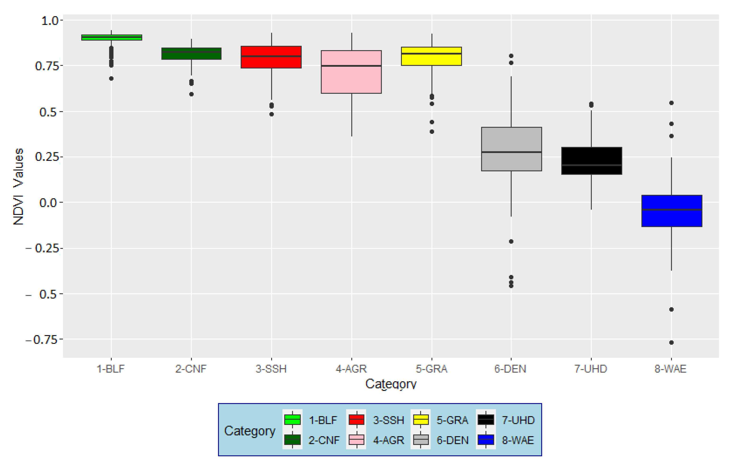
| 1 | Broadleaf forest (BLF) | Vegetation formation composed mainly of mature trees with shrub and undergrowth presence in which broadleaved species predominate. Applicable to mature forests of natural or anthropogenic origin such as pure or mixed broadleaved stands; riparian and gallery forests; broadleaved deciduous thermophiles forests; evergreen sclerophyllous forests; arborescent thickets with sclerophyllous broadleaved species; logging areas; young broadleaved tree plantations; also, to young broadleaved plantations. |
| 2 | Coniferous forest (CNF) | Vegetation formation consisting of mature trees with shrub and undergrowth presence in which coniferous species predominate. Applicable to mature forests of natural or anthropogenic origin such as pure or mixed coniferous stands; deciduous, coniferous forest; arborescent scrub. Furthermore, to young conifer plantations and coniferous wooded dunes. |
| 3 | Shrublands (SSH) | Areas of dense, herbaceous vegetation with occasional scattered trees. Representative of natural development of broadleaved and/or coniferous forest formations in transition by natural succession on abandoned agricultural land; forest regeneration after damage (fire, landslides); stages of forest degeneration caused by natural or anthropogenic stress factors; reforestation after logging or planting in previously non-forested natural or semi-natural areas. |
| 4 | Agricultural land, crops (AGR) | Areas of cultivated land in agricultural use for arable crops irrigated periodically or permanently, using permanent infrastructure (irrigation channels, drainage network and additional irrigation facilities). Most of these crops cannot be cultivated without an artificial water supply. |
| 5 | Pasture and grassland (GRA) | Permanent grasslands characterised by agricultural use or heavy human disturbance. They have a floral composition influenced by human activity, usually grazing or mechanical harvesting of grass meadows. |
| 6 | Denude rock and bare soil (DEN) | Areas of boulders, cliffs, rocky outcrops, including areas of active erosion, rocks and natural no vegetated expanses of sand or pebble/gravel. In coastal or inland locations, such as beaches, dunes, gravel, including torrential stream channel beds. It also includes areas with sparse vegetation consisting of herbaceous and/or semi-woody species covering 10–50% of the area. Includes steppes, tundra, lichen heaths, wastelands, karst areas and sparse vegetation at high altitudes. |
| 7 | Urban and human-derived areas (UHD) | Areas of continuous or discontinuous urban land, as well as industrial areas, road networks, port areas and artificial areas occupied by extractive activities. Areas with artificial vegetation are also included. |
| 8 | Water ecosystem (WAE) | Inland sea area and lower tidal limit as well as lakes, ponds and flowing waters formed by all rivers and streams, including also artificial water bodies such as reservoirs and canals. |
| L.U. | 1989 | 2019 | 2049 | ||||||||
|---|---|---|---|---|---|---|---|---|---|---|---|
| Surface (ha) | % Surface | Surface (ha) | % Surface | Surface (ha) | % Surface | ||||||
| BLF | FOR | 36,499.40 | 36,874.69 | 14.69 | 14.84 | 94,517.00 | 96,499.57 | 38.04 | 38.84 | 153,799.57 | 61.89 |
| CNF | 375.29 | 0.15 | 1982.57 | 0.80 | |||||||
| SSH | 99,809.43 | 40.16 | 85,214.25 | 34.29 | 39,627.61 | 15.95 | |||||
| AGR | 21,619.85 | 8.70 | 11,090.19 | 4.46 | 11,090.19 | 4.46 | |||||
| GRA | 57,229.07 | 23.03 | 21,533.37 | 8.67 | 9820.01 | 3.95 | |||||
| DEN | 31,819.08 | 12.80 | 31,449.75 | 12.66 | 31,449.75 | 12.66 | |||||
| UHD | 767.20 | 0.31 | 2332.19 | 0.94 | 2332.19 | 0.94 | |||||
| WAE | 380.01 | 0.15 | 380.01 | 0.15 | 380.01 | 0.15 | |||||
| Erosion at Source | Sediment Transport | Sediment Deposition | Total | ||||
|---|---|---|---|---|---|---|---|
| Low | Medium | High | Very High | ||||
| Forest conservation (ha) | 92.48 | 308.22 | 122.51 | 85.77 | 77.17 | 5.98 | 692.13 |
| Forest restoration (ha) | 137.48 | 556.24 | 185.90 | 108.47 | 236.42 | 64.6 | 1289.14 |
Publisher’s Note: MDPI stays neutral with regard to jurisdictional claims in published maps and institutional affiliations. |
© 2022 by the authors. Licensee MDPI, Basel, Switzerland. This article is an open access article distributed under the terms and conditions of the Creative Commons Attribution (CC BY) license (https://creativecommons.org/licenses/by/4.0/).
Share and Cite
Hernández-Romero, G.; Álvarez-Martínez, J.M.; Pérez-Silos, I.; Silió-Calzada, A.; Vieites, D.R.; Barquín, J. From Forest Dynamics to Wetland Siltation in Mountainous Landscapes: A RS-Based Framework for Enhancing Erosion Control. Remote Sens. 2022, 14, 1864. https://0-doi-org.brum.beds.ac.uk/10.3390/rs14081864
Hernández-Romero G, Álvarez-Martínez JM, Pérez-Silos I, Silió-Calzada A, Vieites DR, Barquín J. From Forest Dynamics to Wetland Siltation in Mountainous Landscapes: A RS-Based Framework for Enhancing Erosion Control. Remote Sensing. 2022; 14(8):1864. https://0-doi-org.brum.beds.ac.uk/10.3390/rs14081864
Chicago/Turabian StyleHernández-Romero, Gonzalo, Jose Manuel Álvarez-Martínez, Ignacio Pérez-Silos, Ana Silió-Calzada, David R. Vieites, and Jose Barquín. 2022. "From Forest Dynamics to Wetland Siltation in Mountainous Landscapes: A RS-Based Framework for Enhancing Erosion Control" Remote Sensing 14, no. 8: 1864. https://0-doi-org.brum.beds.ac.uk/10.3390/rs14081864