
Evaluating Atmospheric Correction Algorithms Applied to OLCI Sentinel-3 Data of Chesapeake Bay Waters


Abstract
:
1. Introduction
2. Materials and Methods
2.1. Study Area
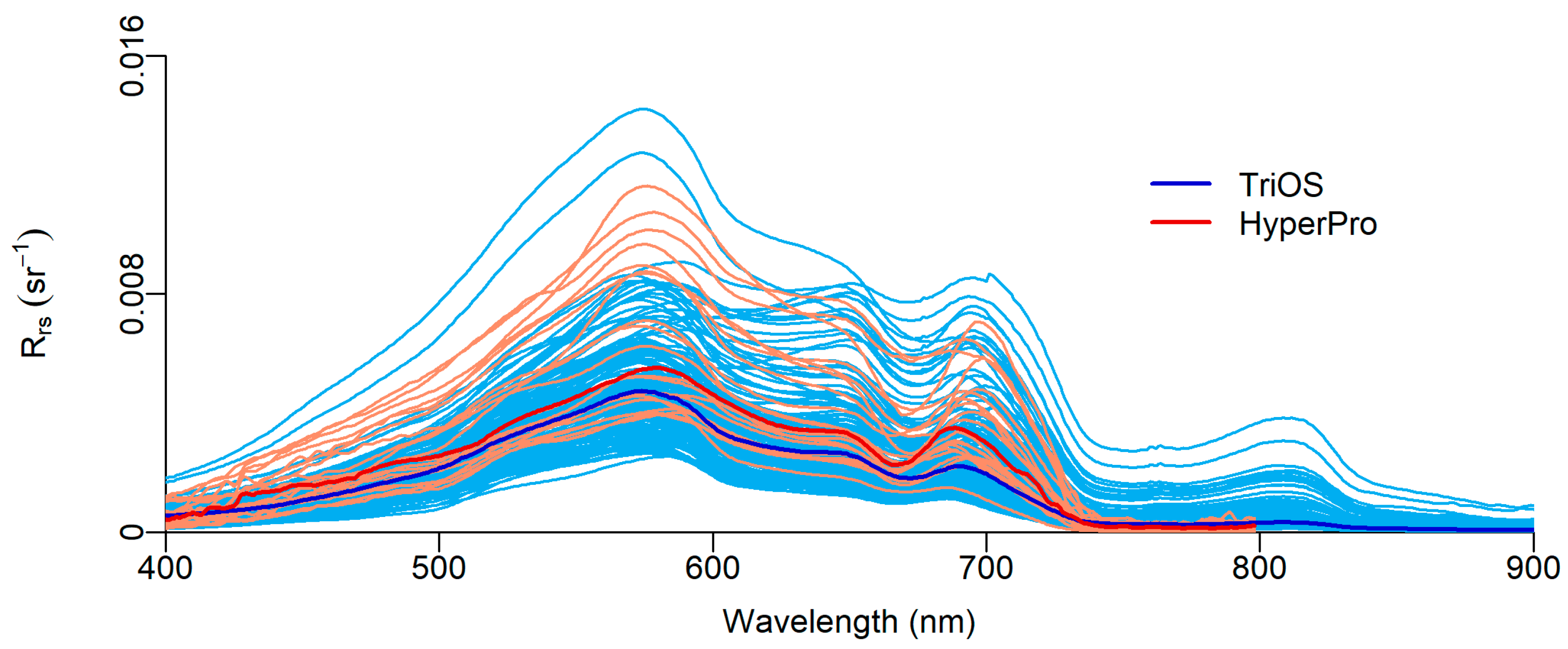
2.2. In Situ Radiometry
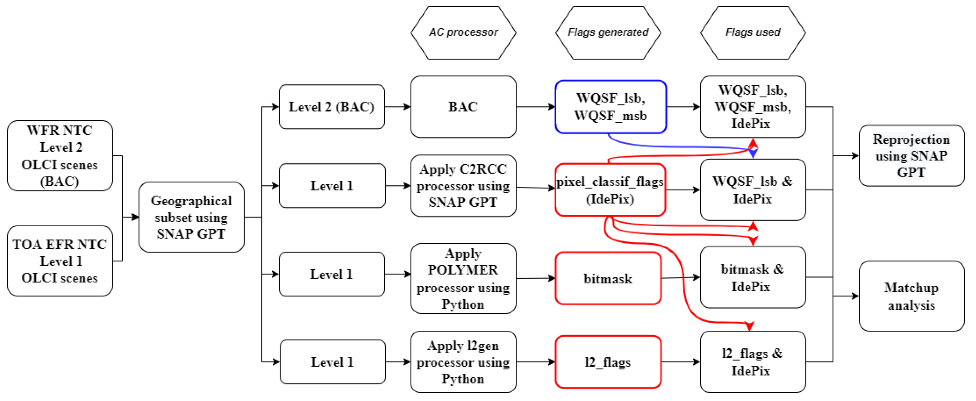
2.3. Satellite Data Collection
2.4. Atmospheric Correction Algorithms
2.5. Match-Up Analysis
2.6. OLCI Composites
3. Results
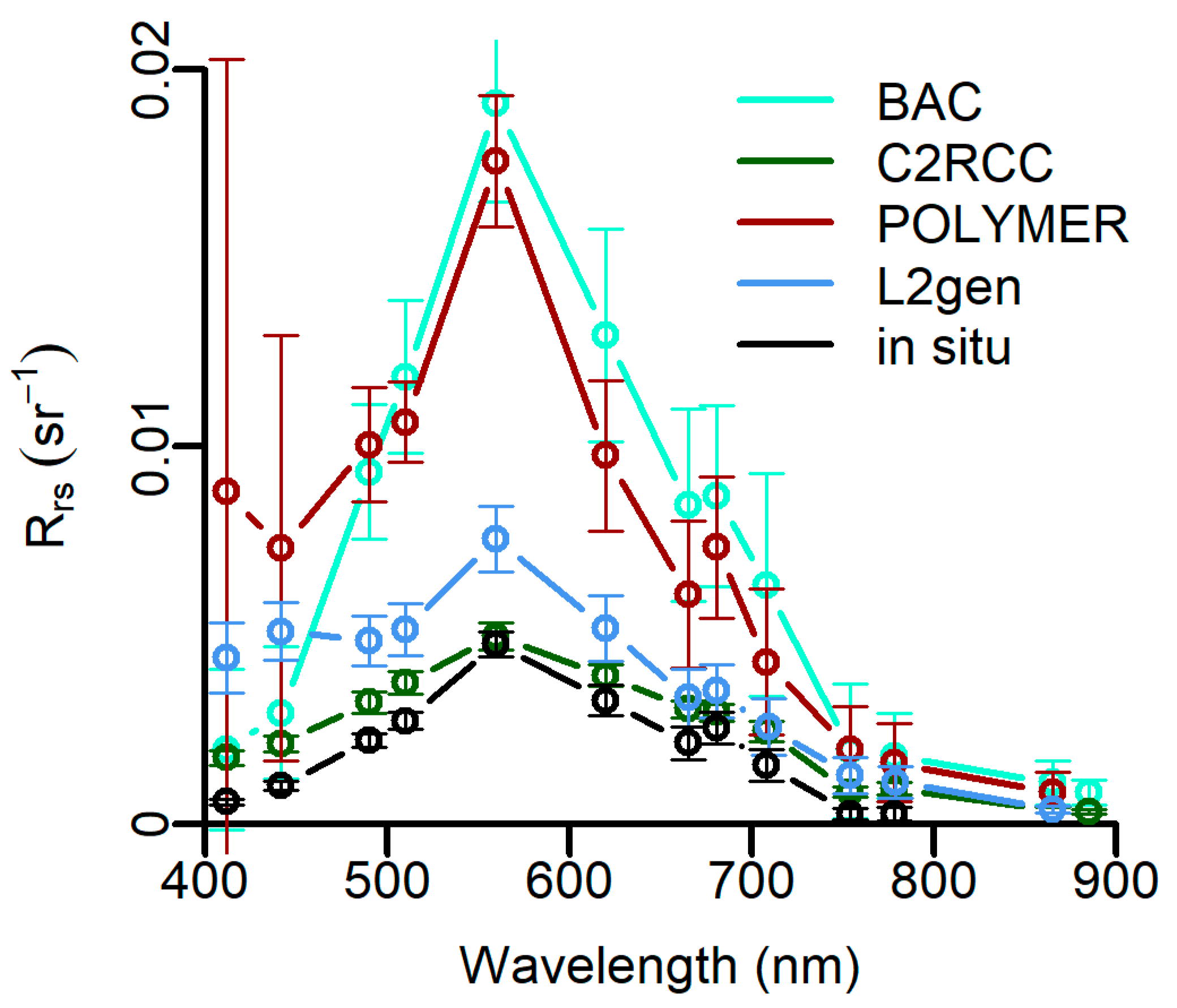
3.1. In Situ and Satellite-Derived Radiometry
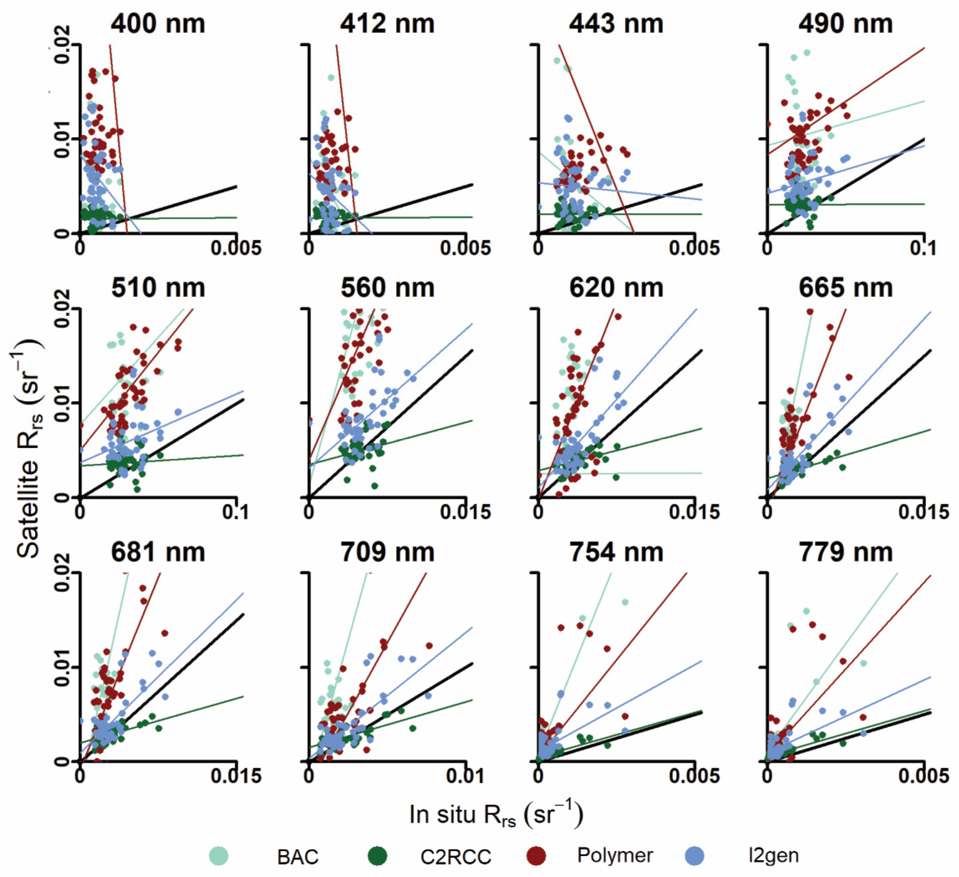
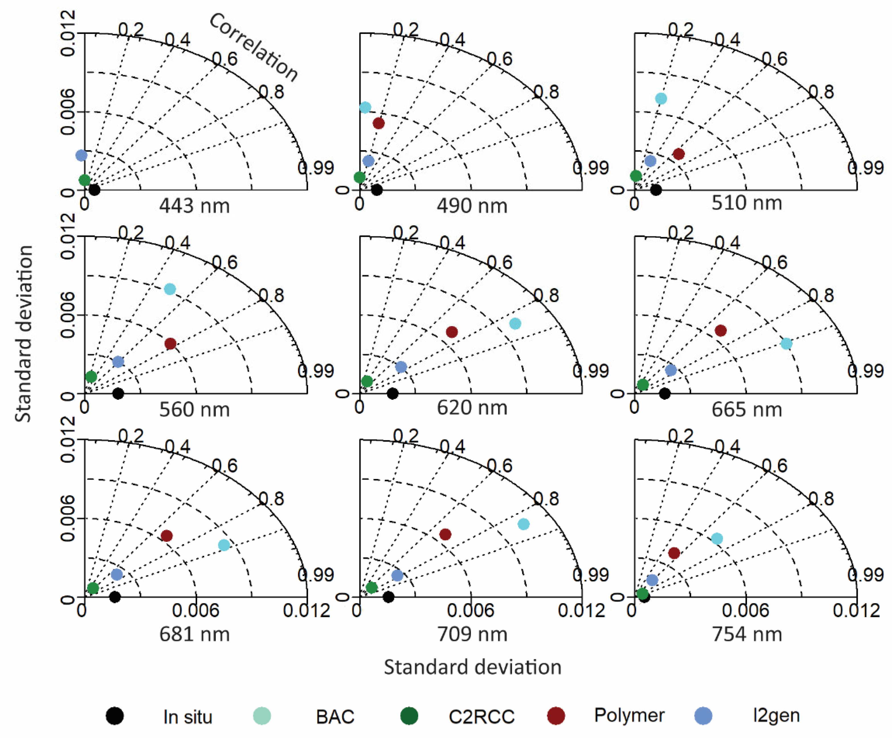
3.2. Matchup Analysis
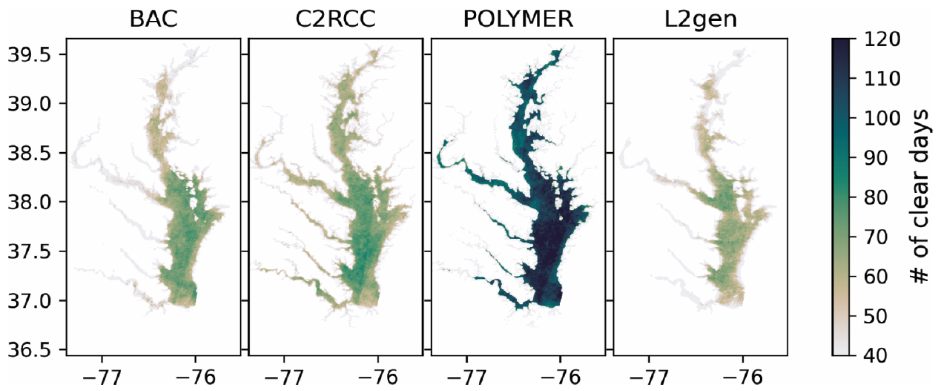
3.3. Pixel Flagging
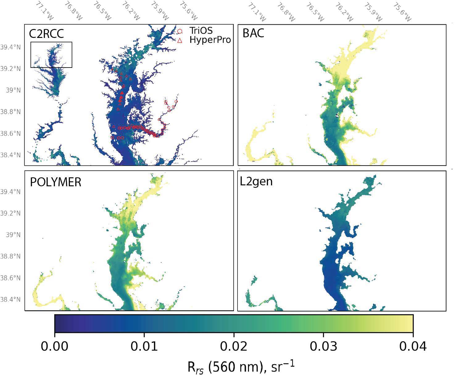
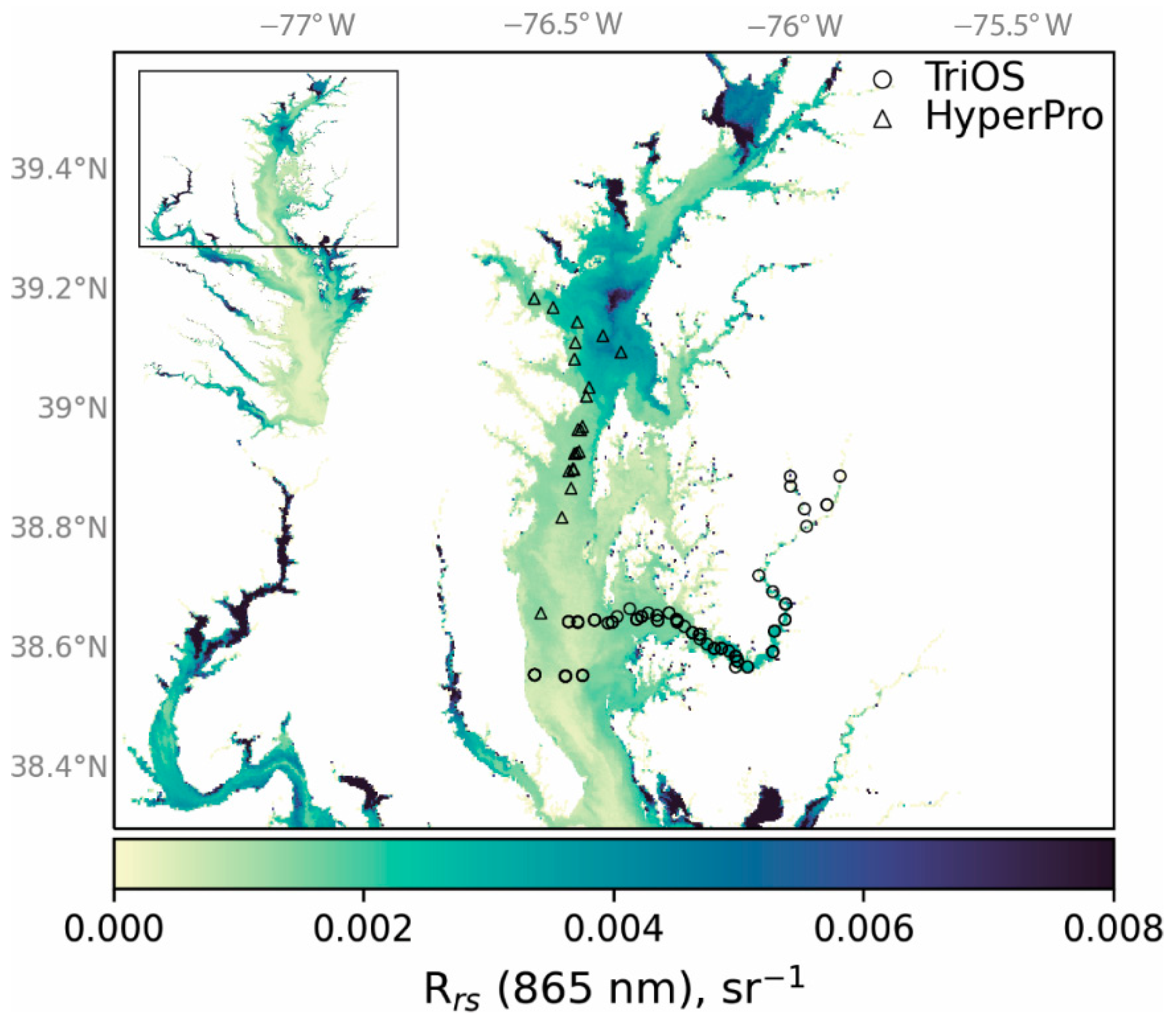
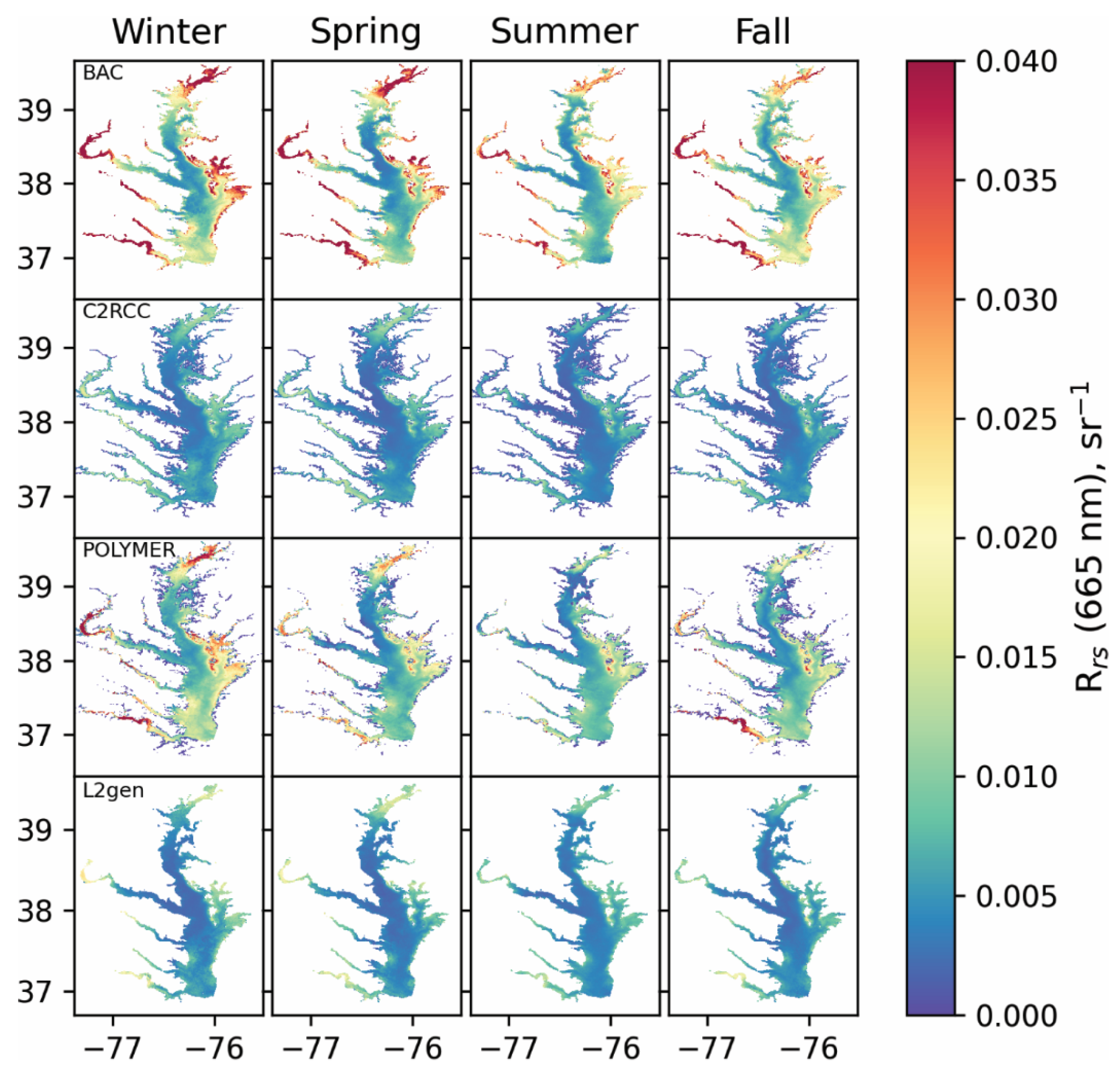
3.4. Rrs Composites
4. Discussion
4.1. Performance of Atmospheric Correction Processors in Chesapeake Bay
4.2. Comparison to Similar Studies
4.3. Matchup Uncertainties
4.4. Pixel Flagging
4.5. Management Implications
4.6. Future Approaches
5. Conclusions
Supplementary Materials
Author Contributions
Funding
Data Availability Statement
Acknowledgments
Conflicts of Interest
References
- IOCCG. Remote Sensing of Inherent Optical Properties: Fundamentals, Tests of Algorithms, and Applications; Lee, Z.-P., Ed.; Reports of the International Ocean-Colour Coordinating Group, No. 5; IOCCG: Dartmouth, NS, Canada, 2006. [Google Scholar]
- O’Reilly, J.E.; Maritorena, S.; Mitchell, B.G.; Siegel, D.A.; Carder, K.L.; Garver, S.A.; Kahru, M.; McClain, C. Ocean Color Chlorophyll Algorithms for SeaWiFS. J. Geophys. Res. Ocean. 1998, 103, 24937–24953. [Google Scholar] [CrossRef] [Green Version]
- Mannino, A.; Russ, M.E.; Hooker, S.B. Algorithm Development and Validation for Satellite-Derived Distributions of DOC and CDOM in the U.S. Middle Atlantic Bight. J. Geophys. Res. Ocean. 2008, 113. [Google Scholar] [CrossRef]
- Lee, Z.P.; Du, K.P.; Arnone, R. A Model for the Diffuse Attenuation Coefficient of Downwelling Irradiance. J. Geophys. Res. C Ocean. 2005, 110, 1–10. [Google Scholar] [CrossRef]
- Nechad, B.; Ruddick, K.G.; Park, Y. Calibration and Validation of a Generic Multisensor Algorithm for Mapping of Total Suspended Matter in Turbid Waters. Remote Sens. Environ. 2010, 114, 854–866. [Google Scholar] [CrossRef]
- Ondrusek, M.; Stengel, E.; Kinkade, C.S.; Vogel, R.L.; Keegstra, P.; Hunter, C.; Kim, C. The Development of a New Optical Total Suspended Matter Algorithm for the Chesapeake Bay. Remote Sens. Environ. 2012, 119, 243–254. [Google Scholar] [CrossRef] [Green Version]
- IOCCG. Atmospheric Correction for Remotely-Sensed Ocean-Colour Products; Wang, M., Ed.; Reports of the International Ocean-Colour Coordinating Group, No. 10; IOCCG: Dartmouth, NS, Canada, 2020. [Google Scholar]
- Mobley, C.D.; Werdell, J.; Franz, B.; Ahmad, Z.; Bailey, S. Atmospheric Correction for Satellite Ocean Color Radiometry; No. GSFC-E-DAA-TN35509; NASA: Washington, DC, USA, 2016. [Google Scholar]
- Ahmad, Z.; Franz, B.A.; McClain, C.R.; Kwiatkowska, E.J.; Werdell, J.; Shettle, E.P.; Holben, B.N. New aerosol models for the retrieval of aerosol optical thickness and normalized water-leaving radiances from the SeaWiFS and MODIS sensors over coastal regions and open oceans. Appl. Opt. 2010, 49, 5545–5560. [Google Scholar] [CrossRef]
- Shettle, E.; Fenn, R.W. Models for the Aerosols of the Lower Atmosphere and the Effects of Humidity Variations on Their Optical Properties. Air Force Geophys. Lab. Air Force Syst. Command United States Air Force 1976, 79, 214. [Google Scholar]
- Gordon, H.R.; Wang, M. Retrieval of Water-Leaving Radiance and Aerosol Optical Thickness over the Oceans with SeaWiFS: A Preliminary Algorithm. Appl. Opt. 1994, 33, 443–452. [Google Scholar] [CrossRef]
- Siegel, D.A.; Wang, M.; Maritorena, S.; Robinson, W. Atmospheric Correction of Satellite Ocean Color Imagery: The Black Pixel Assumption. Appl. Opt. 2000, 39, 3582–3591. [Google Scholar] [CrossRef]
- Gordon, H.R. Removal of Atmospheric Effects from Satellite Imagery of the Oceans. Appl. Opt. 1978, 17, 1631. [Google Scholar] [CrossRef]
- Antoine, D.; Morel, A.; Antoine, D.; Morell, A. A Multiple Scattering Algorithm for Atmospheric Correction of Remotely Sensed Ocean Colour (MERIS Instrument): Principle and Implementation for Atmospheres Carrying Various Aerosols Including Absorbing Ones. Int. J. Remote Sens. 1999, 20, 1875–1916. [Google Scholar] [CrossRef]
- IOCCG. Remote Sensing of Ocean Colour in Coastal, and Other Optically-Complex, Waters; Sathyendranath, S., Ed.; Reports of the International Ocean-Colour Coordinating Group, No. 3; IOCCG: Dartmouth, NS, Canada, 2000. [Google Scholar]
- Ruddick, K.G.; de Cauwer, V.; Park, Y.J.; Moore, G. Seaborne Measurements of near Infrared Water-Leaving Reflectance: The Similarity Spectrum for Turbid Waters. Limnol. Oceanogr. 2006, 51, 1167–1179. [Google Scholar] [CrossRef] [Green Version]
- Mouw, C.B.; Greb, S.; Aurin, D.; DiGiacomo, P.M.; Lee, Z.; Twardowski, M.; Binding, C.; Hu, C.; Ma, R.; Moore, T.; et al. Aquatic color radiometry remote sensing of coastal and inland waters: Challenges and recommendations for future satellite missions. Remote Sens. Environ. 2015, 160, 15–30. [Google Scholar] [CrossRef]
- Zheng, G.; DiGiacomo, P.M. Uncertainties and Applications of Satellite-Derived Coastal Water Quality Products. Prog. Oceanogr. 2017, 159, 45–72. [Google Scholar] [CrossRef]
- Wang, M.; Shi, W. The NIR-SWIR Combined Atmospheric Correction Approach for MODIS Ocean Color Data Processing. Opt. Express 2007, 15, 15722–15733. [Google Scholar] [CrossRef] [Green Version]
- Wang, M. Remote Sensing of the Ocean Contributions from Ultraviolet to Near-Infrared Using the Shortwave Infrared Bands: Simulations. Appl. Opt. 2007, 46, 1535–1547. [Google Scholar] [CrossRef]
- Shi, W.; Wang, M. An Assessment of the Black Ocean Pixel Assumption for MODIS SWIR Bands. Remote Sens. Environ. 2009, 113, 1587–1597. [Google Scholar] [CrossRef]
- Werdell, P.J.; Franz, B.A.; Bailey, S.W. Evaluation of Shortwave Infrared Atmospheric Correction for Ocean Color Remote Sensing of Chesapeake Bay. Remote Sens. Environ. 2010, 114, 2238–2247. [Google Scholar] [CrossRef] [Green Version]
- Vanhellemont, Q.; Ruddick, K. Atmospheric Correction of Sentinel-3/OLCI Data for Mapping of Suspended Particulate Matter and Chlorophyll-a Concentration in Belgian Turbid Coastal Waters. Remote Sens. Environ. 2021, 256, 112284. [Google Scholar] [CrossRef]
- Ibrahim, A.; Franz, B.A.; Ahmad, Z.; Bailey, S.W. Multiband Atmospheric Correction Algorithm for Ocean Color Retrievals. Front. Earth Sci. 2019, 7, 116. [Google Scholar] [CrossRef]
- Ruddick, K.G.; Ovidio, F.; Rijkeboer, M. Atmospheric Correction of SeaWiFS Imagery for Turbid Coastal and Inland Waters. Appl. Opt. 2000, 39, 897–912. [Google Scholar] [CrossRef] [PubMed] [Green Version]
- Goyens, C.; Jamet, C.; Schroeder, T. Evaluation of Four Atmospheric Correction Algorithms for MODIS-Aqua Images over Contrasted Coastal Waters. Remote Sens. Environ. 2013, 131, 63–75. [Google Scholar] [CrossRef]
- Stumpf, R.P.; Arnone, R.A.; Gould, R.W.; Martinolich, P.M.; Ransibrahmanakul, V. A partially coupled ocean-atmosphere model for retrieval of water-leaving radiance from SeaWiFS in coastal waters. NASA Tech. Memo 2003, 206892, 51–59. [Google Scholar]
- Bailey, S.W.; Franz, B.A.; Werdell, P.J. Estimation of near-infrared water-leaving reflectance for satellite ocean color data processing. Opt. Express 2010, 18, 7521–7527. [Google Scholar] [CrossRef] [PubMed]
- Lavender, S.J.; Pinkerton, M.H.; Moore, G.F.; Aiken, J.; Blondeau-Patissier, D. Modification to the Atmospheric Correction of SeaWiFS Ocean Colour Images over Turbid Waters. Cont. Shelf Res. 2005, 25, 539–555. [Google Scholar] [CrossRef]
- Schroeder, T.; Behnert, I.; Schaale, M.; Fischer, J.; Doerffer, R.; Schroeder, T.H.; Behnert, I.; Schaale, M.; Fischer, J.; Doerffer, R. Atmospheric Correction Algorithm for MERIS above Case-2 Waters. Int. J. Remote Sens. 2007, 28, 1469–1486. [Google Scholar] [CrossRef]
- Doerffer, R.; Schiller, H. The MERIS Case 2 Water Algorithm. Int. J. Remote Sens. 2007, 28, 517–535. [Google Scholar] [CrossRef]
- Kuchinke, C.P.; Gordon, H.R.; Franz, B.A. Spectral Optimization for Constituent Retrieval in Case 2 Waters I: Implementation and Performance. Remote Sens. Environ. 2009, 113, 571–587. [Google Scholar] [CrossRef]
- Steinmetz, F.; Deschamps, P.Y.; Ramon, D. Atmospheric correction in presence of sun glint: Application to MERIS. Opt. Express 2011, 19, 9783–9800. [Google Scholar] [CrossRef] [Green Version]
- Hieronymi, M.; Müller, D.; Doerffer, R. The OLCI Neural Network Swarm (ONNS): A Bio-Geo-Optical Algorithm for Open Ocean and Coastal Waters. Front. Mar. Sci. 2017, 4, 140. [Google Scholar] [CrossRef] [Green Version]
- Mograne, M.; Jamet, C.; Loisel, H.; Vantrepotte, V.; Mériaux, X.; Cauvin, A. Evaluation of Five Atmospheric Correction Algorithms over French Optically-Complex Waters for the Sentinel-3A OLCI Ocean Color Sensor. Remote Sens. 2019, 11, 668. [Google Scholar] [CrossRef] [Green Version]
- Gossn, J.I.; Ruddick, K.G.; Dogliotti, A.I. Atmospheric Correction of OLCI Imagery over Extremely Turbid Waters Based on the Red, NIR and 1016 Nm Bands and a New Baseline Residual Technique. Remote Sens. 2019, 11, 220. [Google Scholar] [CrossRef] [Green Version]
- Kyryliuk, D.; Kratzer, S. Evaluation of Sentinel-3A OLCI Products Derived Using the Case-2 Regional Coastcolour Processor over the Baltic Sea. Sensors 2019, 19, 3609. [Google Scholar] [CrossRef] [PubMed] [Green Version]
- Pereira-Sandoval, M.; Ruescas, A.; Urrego, P.; Ruiz-Verdú, A.; Delegido, J.; Tenjo, C.; Soria-Perpinyà, X.; Vicente, E.; Soria, J.; Moreno, J. Evaluation of Atmospheric Correction Algorithms over Spanish Inland Waters for Sentinel-2 Multi Spectral Imagery Data. Remote Sens. 2019, 11, 1469. [Google Scholar] [CrossRef] [Green Version]
- Renosh, P.R.; Doxaran, D.; de Keukelaere, L.; Gossn, J.I. Evaluation of Atmospheric Correction Algorithms for Sentinel-2-MSI and Sentinel-3-OLCI in Highly Turbid Estuarine Waters. Remote Sens. 2020, 12, 1285. [Google Scholar] [CrossRef] [Green Version]
- Giannini, F.; Hunt, B.P.V.; Jacoby, D.; Costa, M. Performance of OLCI Sentinel-3A Satellite in the Northeast Pacific Coastal Waters. Remote Sens. Environ. 2021, 256, 112317. [Google Scholar] [CrossRef]
- Kemp, W.M.; Boynton, W.R.; Adolf, J.E.; Boesch, D.F.; Boicourt, W.C.; Brush, G.; Cornwell, J.C.; Fisher, T.R.; Glibert, P.M.; Hagy, J.D.; et al. Eutrophication of Chesapeake Bay: Historical Trends and Ecological Interactions. Mar. Ecol. Prog. Ser. 2005, 303, 1–29. [Google Scholar] [CrossRef]
- Miller, W.D.; Kimmel, D.G.; Harding, L.W. Predicting Spring Discharge of the Susquehanna River from a Winter Synoptic Climatology for the Eastern United States. Water Resour. Res. 2006, 42. [Google Scholar] [CrossRef] [Green Version]
- Harding, L.W.; Magnuson, A.; Mallonee, M.E. SeaWiFS Retrievals of Chlorophyll in Chesapeake Bay and the Mid-Atlantic Bight. Estuar. Coast. Shelf Sci. 2005, 62, 75–94. [Google Scholar] [CrossRef]
- Tzortziou, M.; Subramaniam, A.; Herman, J.R.; Gallegos, C.L.; Neale, P.J.; Harding, L.W. Remote Sensing Reflectance and Inherent Optical Properties in the Mid Chesapeake Bay. Estuar. Coast. Shelf Sci. 2007, 72, 16–32. [Google Scholar] [CrossRef]
- Froidefond, J.-M.; Ouillon, S. Introducing a Mini-Catamaran to Perform Reflectance Measurements above and below the Water Surface. Opt. Express 2015, 13, 926–936. [Google Scholar] [CrossRef] [PubMed]
- Ahn, Y.H.; Ryu, J.H.; Moon, J.E. Development of Red tide & Water Turbidity Algorithms Using Ocean Color Satellite; Report No. BSPE 98721-00-1224-01; KORDI: Seoul, Korea, 1999. [Google Scholar]
- Lee, Z.; Pahlevan, N.; Ahn, Y.H.; Greb, S.; O’Donnell, D. Robust approach to directly measuring water-leaving radiance in the field. Appl. Opt. 2013, 52, 1693–1701. [Google Scholar] [CrossRef] [PubMed]
- Lee, Z.; Wei, J.; Shang, Z.; Garcia, R.; Dierssen, H.M.; Ishizaka, J.; Castagna, A. On-water radiometry measurements: Skylight-blocked approach and data processing. Appendix to Protocols for Satellite Ocean Colour Data Validation: In Situ Optical Radiometry. IOCCG Ocean Opt. Biogeochem. Protoc. Satell. Ocean Colour Sens. Valid. 2019, 3, 7. [Google Scholar]
- Ondrusek, M.E.; Stengel, E.; Rella, M.A.; Goode, W.; Ladner, S.; Feinholz, M. Validation of ocean color sensors using a profiling hyperspectral radiometer. In Ocean Sensing and Monitoring VI; International Society for Optics and Photonics: Bellingham, WA, USA, 2014; Volume 9111, p. 91110Y. [Google Scholar]
- EUMETSAT. Sentinel-3 OLCI Marine User Handbook 2018. Available online: https://earth.esa.int/eogateway/documents/20142/1564943/Sentinel-3-OLCI-Marine-User-Handbook.pdf (accessed on 13 March 2022).
- Moore, G.F.; Aiken, J.; Lavender, S.J. The Atmospheric Correction of Water Colour and the Quantitative Retrieval of Suspended Particulate Matter in Case II Waters: Application to MERIS. Int. J. Remote Sens. 1999, 20, 1713–1733. [Google Scholar] [CrossRef]
- Moore, G.F.; Mazeran, C.; Huot, J.P. Case II.S Bright Pixel Atmospheric Correction; MERIS Algorithm Theoretical. Basis Document (ATBD) 2.6; MERIS ATBD-ESA Earth Online: Frascati, Italy, 2017; p. 82. [Google Scholar]
- Barker, K.; Mazeran, C.; Lerebourg, C.; Bouvet, M.; Antoine, D.; Ondrusek, M.; Zibordi, G.; Lavender, S. Mermaid: The MERIS matchup in-situ database. In Proceedings of the 2nd (A) ATSR and MERIS Workshop, Frascati, Italy, 22–26 September 2008. [Google Scholar]
- Mobley, C. Light and Water: Radiative Transfer in Natural Waters; Academic: San Diego, CA, USA, 1994. [Google Scholar]
- Brockmann, C.; Doerffer, R.; Peters, M.; Kerstin, S.; Embacher, S.; Ruescas, A. Evolution of the C2RCC neural network for Sentinel 2 and 3 for the retrieval of ocean colour products in normal and extreme optically complex waters. In Proceedings of the Living Planet Symposium, Prague, Czech Republic, 9–13 May 2016; Volume 740, p. 54. [Google Scholar]
- Soppa, M.A.; Silva, B.; Steinmetz, F.; Keith, D.; Scheffler, D.; Bohn, N.; Bracher, A. Assessment of Polymer Atmospheric Correction Algorithm for Hyperspectral Remote Sensing Imagery over Coastal Waters. Sensors 2021, 21, 4125. [Google Scholar] [CrossRef]
- Steinmetz, F.; Ramon, D. Sentinel-2 MSI and Sentinel-3 OLCI Consistent Ocean Colour Products Using POLYMER. In Remote Sensing of the Open and Coastal Ocean and Inland Waters; International Society for Optics and Photonics: Bellingham, WA, USA, 2018; Volume 10778, p. 107780E. [Google Scholar] [CrossRef]
- Kratzer, S.; Plowey, M. Integrating Mooring and Ship-Based Data for Improved Validation of OLCI Chlorophyll-a Products in the Baltic Sea. Int. J. Appl. Earth Obs. Geoinf. 2021, 94, 102212. [Google Scholar] [CrossRef]
- Sathyendranath, S.; Brewin, R.J.; Brockmann, C.; Brotas, V.; Calton, B.; Chuprin, A.; Cipollini, P.; Couto, A.B.; Dingle, J.; Doerffer, R.; et al. An Ocean-Colour Time Series for Use in Climate Studies: The Experience of the Ocean-Colour Climate Change Initiative (OC-CCI). Sensors 2019, 19, 4285. [Google Scholar] [CrossRef] [Green Version]
- EUMETSAT. Sentinel-3 OLCI L2 Report for Baseline Collection OL_L2M_003. 2021. Available online: https://www.eumetsat.int/media/47794 (accessed on 13 March 2022).
- Taylor, K.E. Summarizing Multiple Aspects of Model Performance in a Single Diagram. J. Geophys. Res. Atmos. 2001, 106, 7183–7192. [Google Scholar] [CrossRef]
- Jolliff, J.K.; Kindle, J.C.; Shulman, I.; Penta, B.; Friedrichs, M.A.; Helber, R.; Arnone, R.A. Summary Diagrams for Coupled Hydrodynamic-Ecosystem Model Skill Assessment. J. Mar. Syst. 2009, 76, 64–82. [Google Scholar] [CrossRef]
- Gitelson, A.A.; Schalles, J.F.; Hladik, C.M. Remote Chlorophyll-a Retrieval in Turbid, Productive Estuaries: Chesapeake Bay Case Study. Remote Sens. Environ. 2007, 109, 464–472. [Google Scholar] [CrossRef]
- Gitelson, A.A.; Dall’Olmo, G.; Moses, W.; Rundquist, D.C.; Barrow, T.; Fisher, T.R.; Gurlin, D.; Holz, J. A Simple Semi-Analytical Model for Remote Estimation of Chlorophyll-a in Turbid Waters: Validation. Remote Sens. Environ. 2008, 112, 3582–3593. [Google Scholar] [CrossRef]
- Spyrakos, E.; O’donnell, R.; Hunter, P.D.; Miller, C.; Scott, M.; Simis, S.G.; Neil, C.; Barbosa, C.C.; Binding, C.E.; Bradt, S.; et al. Optical Types of Inland and Coastal Waters. Limnol. Oceanogr. 2018, 63, 846–870. [Google Scholar] [CrossRef] [Green Version]
- Frouin, R.J.; Franz, B.A.; Ibrahim, A.; Knobelspiesse, K.; Ahmad, Z.; Cairns, B.; Chowdhary, J.; Dierssen, H.M.; Tan, J.; Dubovik, O.; et al. Atmospheric Correction of Satellite Ocean-Color Imagery During the PACE Era. Front. Earth Sci. 2019, 7. [Google Scholar] [CrossRef] [Green Version]
- Son, S.H.; Wang, M. Water Properties in Chesapeake Bay from MODIS-Aqua Measurements. Remote Sens. Environ. 2012, 123, 163–174. [Google Scholar] [CrossRef] [Green Version]
- Gons, H.J.; Rijkeboer, M.; Ruddick, K.G. A Chlorophyll-Retrieval Algorithm for Satellite Imagery (Medium Resolution Imaging Spectrometer) of Inland and Coastal Waters. J. Plankton Res. 2002, 24, 947–951. [Google Scholar] [CrossRef] [Green Version]
- Moses, W.J.; Saprygin, V.; Gerasyuk, V.; Povazhnyy, V.; Berdnikov, S.; Gitelson, A.A. OLCI-Based NIR-Red Models for Estimating Chlorophyll-a Concentration in Productive Coastal Waters—A Preliminary Evaluation. Environ. Res. Commun. 2019, 1, 011002. [Google Scholar] [CrossRef]
- Zibordi, G.; Holben, B.N.; Talone, M.; D’Alimonte, D.; Slutsker, I.; Giles, D.M.; Sorokin, M.G. Advances in the Ocean Color Component of the Aerosol Robotic Network (AERONET-OC). J. Atmos. Ocean. Technol. 2021, 38, 725–746. [Google Scholar] [CrossRef]
- Alikas, K.; Ansko, I.; Vabson, V.; Ansper, A.; Kangro, K.; Uudeberg, K.; Ligi, M. Consistency of Radiometric Satellite Data over Lakes and Coastalwaters with Local Field Measurements. Remote Sens. 2020, 12, 616. [Google Scholar] [CrossRef] [Green Version]
- Xue, K.; Ma, R.; Shen, M.; Li, Y.; Duan, H.; Cao, Z.; Wang, D.; Xiong, J. Variations of Suspended Particulate Concentration and Composition in Chinese Lakes Observed from Sentinel-3A OLCI Images. Sci. Total Environ. 2020, 721, 137774. [Google Scholar] [CrossRef]
- Schroeder, T.; Schaale, M.; Lovell, J.; Blondeau-Patissier, D. An Ensemble Neural Network Atmospheric Correction for Sentinel-3 OLCI over Coastal Waters Providing Inherent Model Uncertainty Estimation and Sensor Noise Propagation. Remote Sens. Environ. 2022, 270, 112848. [Google Scholar] [CrossRef]
- Zibordi, G.; Ruddick, K.; Ansko, I.; Moore, G.; Kratzer, S.; Icely, J.; Reinart, A. In Situ Determination of the Remote Sensing Reflectance: An Inter-Comparison. Ocean Sci. 2012, 8, 567–586. [Google Scholar] [CrossRef] [Green Version]
- Shang, Z.; Lee, Z.; Dong, Q.; Wei, J. Self-Shading Associated with a Skylight-Blocked Approach System for the Measurement of Water-Leaving Radiance and Its Correction. Appl. Opt. 2017, 56, 7033. [Google Scholar] [CrossRef] [PubMed]
- Ruddick, K.G.; Voss, K.; Boss, E.; Castagna, A.; Frouin, R.; Gilerson, A.; Hieronymi, M.; Johnson, B.C.; Kuusk, J.; Lee, Z.; et al. A Review of Protocols for Fiducial Reference Measurements of Water-Leaving Radiance for Validation of Satellite Remote-Sensing Data over Water. Remote Sens. 2019, 11, 2198. [Google Scholar] [CrossRef] [Green Version]
- Vabson, V.; Kuusk, J.; Ansko, I.; Vendt, R.; Alikas, K.; Ruddick, K.; Ansper, A.; Bresciani, M.; Burmester, H.; Costa, M.; et al. Field Intercomparison of Radiometers Used for Satellite Validation in the 400–900 Nm Range. Remote Sens. 2019, 11, 1129. [Google Scholar] [CrossRef] [Green Version]
- Tilstone, G.; Dall’Olmo, G.; Hieronymi, M.; Ruddick, K.; Beck, M.; Ligi, M.; Costa, M.; D’alimonte, D.; Vellucci, V.; Vansteenwegen, D.; et al. Field Intercomparison of Radiometer Measurements for Ocean Colour Validation. Remote Sens. 2020, 12, 1587. [Google Scholar] [CrossRef]
- Alikas, K.; Vabson, V.; Ansko, I.; Tilstone, G.H.; Dall’Olmo, G.; Nencioli, F.; Vendt, R.; Donlon, C.; Casal, T. Comparison of Above-Water Seabird and TriOS Radiometers along an Atlantic Meridional Transect. Remote Sens. 2020, 12, 1669. [Google Scholar] [CrossRef]
- Antoine, D.; Slivkoff, M.; Klonowski, W.; Kovach, C.; Ondrusek, M. Uncertainty Assessment of Unattended Above-Water Radiometric Data Collection from Research Vessels with the Dynamic Above-Water Radiance (L) and Irradiance (E) Collector (DALEC). Opt. Express 2021, 29, 4607. [Google Scholar] [CrossRef]
- Morel, A.; Antoine, D.; Gentili, B. Bidirectional Reflectance of Oceanic Waters: Accounting for Raman Emission and Varying Particle Scattering Phase Function. Appl. Opt. 2002, 41, 6289. [Google Scholar] [CrossRef]
- Voss, K.J.; Morel, A.; Antoine, D. Detailed Validation of the Bidirectional Effect in Various Case 1 Waters for Application to Ocean Color Imagery. Biogeosciences 2007, 4, 781–789. [Google Scholar] [CrossRef] [Green Version]
- Gilerson, A.; Hlaing, S.; Harmel, T.; Tonizzo, A.; Arnone, R.; Weidemann, A.; Ahmed, S. Bidirectional Reflectance Function in Coastal Waters: Modeling and Validation. In Remote Sensing of the Ocean, Sea Ice, Coastal Waters, and Large Water Regions; SPIE: Bellingham, DC, USA, 2011; Volume 8175, p. 81750. [Google Scholar]
- Fan, Y.; Li, W.; Voss, K.J.; Gatebe, C.K.; Stamnes, K. A Neural Network Method to Correct Bidirectional Effects in Water-Leaving Radiance. In Proceedings of the AIP Conference Proceedings; American Institute of Physics Inc.: College Park, MD, USA, 2018; Volume 1810. [Google Scholar]
- Franz, B.A.; Bailey, S.W.; Werdell, P.J.; McClain, C.R. Sensor-Independent Approach to the Vicarious Calibration of Satellite Ocean Color Radiometry. Appl. Optics. 2007, 46, 5068–5082. [Google Scholar] [CrossRef]
- Hu, C.; Barnes, B.B.; Feng, L.; Wang, M.; Jiang, L. On the Interplay between Ocean Color Data Quality and Data Quantity: Impacts of Quality Control Flags. IEEE Geosci. Remote Sens. Lett. 2020, 17, 745–749. [Google Scholar] [CrossRef]
- Feng, L.; Hu, C. Land Adjacency Effects on MODIS Aqua Top-of-Atmosphere Radiance in the Shortwave Infrared: Statistical Assessment and Correction. J. Geophys. Res. Ocean. 2017, 122, 4802–4818. [Google Scholar] [CrossRef]
- Harding, L.W.; Mallonee, M.E.; Perry, E.S.; Miller, W.D.; Adolf, J.E.; Gallegos, C.L.; Paerl, H.W. Long-Term Trends, Current Status, and Transitions of Water Quality in Chesapeake Bay. Sci. Rep. 2019, 9, 1–19. [Google Scholar] [CrossRef] [PubMed]
- Glibert, P.M. Harmful Algae at the Complex Nexus of Eutrophication and Climate Change. Harmful Algae 2020, 91, 101583. [Google Scholar] [CrossRef]
- Wolny, J.L.; Tomlinson, M.C.; Schollaert Uz, S.; Egerton, T.A.; McKay, J.R.; Meredith, A.; Reece, K.S.; Scott, G.P.; Stumpf, R.P. Current and Future Remote Sensing of Harmful Algal Blooms in the Chesapeake Bay to Support the Shellfish Industry. Front. Mar. Sci. 2020, 7, 337. [Google Scholar] [CrossRef]
- Feng, L.; Hou, X.; Li, J.; Zheng, Y. Exploring the Potential of Rayleigh-Corrected Reflectance in Coastal and Inland Water Applications: A Simple Aerosol Correction Method and Its Merits. ISPRS J. Photogramm. Remote Sens. 2018, 146, 52–64. [Google Scholar] [CrossRef]
- Tomlinson, M.C.; Stumpf, R.P.; Vogel, R.L. Approximation of Diffuse Attenuation, Kd, for MODIS High-Resolution Bands. Remote Sens. Lett. 2019, 10, 178–185. [Google Scholar] [CrossRef]
- Turner, J.S.; Friedrichs, C.T.; Friedrichs, M.A.M. Long-Term Trends in Chesapeake Bay Remote Sensing Reflectance: Implications for Water Clarity. J. Geophys. Res. Ocean. 2021, 126, e2021JC017959. [Google Scholar] [CrossRef]
- Aurin, D.; Mannino, A.; Franz, B. Spatially Resolving Ocean Color and Sediment Dispersion in River Plumes, Coastal Systems, and Continental Shelf Waters. Remote Sens. Environ. 2013, 137, 212–225. [Google Scholar] [CrossRef] [Green Version]
- Werdell, P.J.; Behrenfeld, M.J.; Bontempi, P.S.; Boss, E.; Cairns, B.; Davis, G.T.; Franz, B.A.; Gliese, U.B.; Gorman, E.T.; Hasekamp, O.; et al. The Plankton, Aerosol, Cloud, Ocean Ecosystem Mission Status, Science, Advances. Bull. Am. Meteorol. Soc. 2019, 100, 1775–1794. [Google Scholar] [CrossRef]
- Liu, J.; He, X.; Liu, J.; Bai, Y.; Wang, D.; Chen, T.; Wang, Y.; Zhu, F. Polarization-Based Enhancement of Ocean Color Signal for Estimating Suspended Particulate Matter: Radiative Transfer Simulations and Laboratory Measurements. Opt. Express 2017, 25, A323. [Google Scholar] [CrossRef] [PubMed]


| BAC (n = 27) | C2RCC (n = 41) | |||||||||||
| λ (nm) | Slope | Int | r2 | RMSE (sr−1) | MD (sr−1) | MPD | Slope | Int | r2 | RMSE (sr−1) | MD (sr−1) | MPD |
| 400 | −7.97 | 0.009 | 0.07 | 0.009 | 0.002 | 1470 | 0.03 | 0.002 | 0 | 0.001 | 0.001 | 303 |
| 412 | −5.73 | 0.008 | 0.05 | 0.008 | 0.001 | 1130 | 0.02 | 0.002 | 0 | 0.001 | 0.001 | 236 |
| 443 | −2.8 | 0.009 | 0.03 | 0.008 | 0.002 | 548 | 0.01 | 0.002 | 0 | 0.001 | 0.001 | 119 |
| 490 | 0.47 | 0.009 | 0 | 0.010 | 0.006 | 397 | 0 | 0.003 | 0 | 0.002 | 0.001 | 64 |
| 510 | 1.85 | 0.008 | 0.04 | 0.013 | 0.008 | 365 | 0.11 | 0.003 | 0.01 | 0.002 | 0.001 | 47 |
| 560 | 4.01 | 0.001 | 0.25 | 0.018 | 0.014 | 333 | 0.3 | 0.004 | 0.08 | 0.002 | 0 | 24 |
| 620 | 5.89 | −0.006 | 0.71 | 0.015 | 0.009 | 311 | 0.28 | 0.003 | 0.16 | 0.001 | 0 | 29 |
| 665 | 5.43 | −0.003 | 0.82 | 0.012 | 0.006 | 230 | 0.33 | 0.002 | 0.32 | 0.001 | 0 | 34 |
| 681 | 4.93 | −0.003 | 0.78 | 0.011 | 0.006 | 298 | 0.32 | 0.002 | 0.3 | 0.001 | 0 | 30 |
| 709 | 5.98 | −0.002 | 0.72 | 0.013 | 0.005 | 396 | 0.48 | 0.002 | 0.47 | 0.001 | 0.001 | 51 |
| 754 | 8.22 | 0.001 | 0.5 | 0.007 | 0.002 | 1043 | 0.94 | 0.001 | 0.72 | 0.001 | 0 | 249 |
| 779 | 4.52 | 0.001 | 0.48 | 0.005 | 0.002 | 774 | 0.95 | 0.001 | 0.7 | 0.001 | 0.001 | 378 |
| Mean | 2.07 | 0.003 | 0.37 | 0.011 | 0.010 | 608 | 0.31 | 0.002 | 0.23 | 0.001 | 0.001 | 130 |
| POLYMER (n = 48) | L2gen (n = 46) | |||||||||||
| λ (nm) | Slope | Int | r2 | RMSE (sr−1) | MD (sr−1) | MPD | Slope | Int | r2 | RMSE (sr−1) | MD (sr−1) | MPD |
| 400 | −36.28 | 0.054 | 0.04 | 0.060 | 0.01 | 9809 | −4.26 | 0.008 | 0.11 | 0.006 | 0.005 | 1514 |
| 412 | −30.19 | 0.041 | 0.05 | 0.046 | 0.008 | 4483 | −3.14 | 0.007 | 0.08 | 0.005 | 0.004 | 790 |
| 443 | −8.32 | 0.024 | 0.05 | 0.024 | 0.006 | 1403 | −0.34 | 0.006 | 0.01 | 0.005 | 0.004 | 394 |
| 490 | 1.13 | 0.008 | 0.04 | 0.010 | 0.008 | 395 | 0.5 | 0.004 | 0.04 | 0.004 | 0.003 | 154 |
| 510 | 2.08 | 0.005 | 0.43 | 0.009 | 0.008 | 277 | 0.73 | 0.003 | 0.13 | 0.004 | 0.002 | 103 |
| 560 | 2.54 | 0.003 | 0.6 | 0.013 | 0.012 | 233 | 0.98 | 0.002 | 0.36 | 0.004 | 0.003 | 60 |
| 620 | 2.8 | −0.001 | 0.53 | 0.009 | 0.006 | 192 | 1.25 | 0 | 0.55 | 0.003 | 0.002 | 55 |
| 665 | 2.85 | −0.001 | 0.49 | 0.007 | 0.004 | 205 | 1.21 | 0.001 | 0.55 | 0.002 | 0.001 | 59 |
| 681 | 2.71 | −0.001 | 0.47 | 0.007 | 0.005 | 194 | 1.08 | 0.001 | 0.51 | 0.002 | 0.001 | 51 |
| 709 | 2.98 | −0.002 | 0.49 | 0.006 | 0.003 | 196 | 1.33 | 0 | 0.61 | 0.002 | 0.001 | 667 |
| 754 | 4.12 | 0.001 | 0.29 | 0.004 | 0.002 | 1122 | 1.84 | 0.001 | 0.35 | 0.002 | 0.001 | 719 |
| 779 | 3.65 | 0.001 | 0.35 | 0.004 | 0.001 | 1059 | 1.54 | 0.001 | 0.39 | 0.002 | 0.001 | 757 |
| Mean | −4.16 | 0.011 | 0.32 | 0.017 | 0.006 | 1631 | 0.23 | 0.003 | 0.31 | 0.003 | 0.002 | 444 |
| 443 | 560 | 665 | 754 | ||||||||||
|---|---|---|---|---|---|---|---|---|---|---|---|---|---|
| n | r2 | MD | MPD | r2 | MD | MPD | r2 | MD | MPD | r2 | MD | MPD | |
| This study | |||||||||||||
| BAC | 27 | 0.03 | 0.002 | 548 | 0.25 | 0.014 | 333 | 0.82 | 0.006 | 230 | 0.50 | 0.002 | 1043 |
| C2RCC | 41 | 0 | 0.001 | 119 | 0.08 | 0 | 24 | 0.32 | 0 | 34 | 0.72 | 0 | 249 |
| POLYMER | 48 | 0.05 | 0.006 | 1403 | 0.60 | 0.012 | 233 | 0.49 | 0.004 | 205 | 0.29 | 0.002 | 1122 |
| L2gen | 46 | 0.01 | 0.004 | 394 | 0.36 | 0.003 | 60 | 0.55 | 0.001 | 59 | 0.35 | 0.001 | 719 |
| Mograne et al., 2019 | |||||||||||||
| BAC | 18 | 0.38 * | -- | −40 * | 0.95 * | -- | −10 * | 0.95 * | -- | −40 * | -- | -- | -- |
| C2RCC | 16 | 0.63 * | -- | −5 * | 0.93 * | -- | 0 * | 0.95 * | -- | −20 * | -- | -- | -- |
| C2R-CCAltNets | 19 | 0.84 * | -- | 15 * | 0.94 * | -- | 10 * | 0.90 * | -- | 5 * | -- | -- | -- |
| POLYMER | 35 | 0.54 * | -- | −18 * | 0.86 * | -- | −12 * | 0.93 * | -- | −18 * | -- | -- | -- |
| L2gen | 17 | 0.50 * | -- | 22 * | 0.98 * | -- | −4 * | 0.98 * | -- | −12 * | -- | -- | -- |
| Alikas et al., 2020 | |||||||||||||
| BAC | 22 | 0.028 | -- | −192 | 0.59 | -- | −2 | -- | -- | 12 | -- | -- | 58 |
| C2RCC | 22 | 0.29 | -- | 64 | 0.6 | -- | 16 | -- | -- | 39 | -- | -- | 122 |
| C2RCC ALTNN | 22 | 0.003 | -- | 50 | 0.37 | -- | 7 | -- | -- | 41 | -- | -- | 72 |
| POLYMER | 22 | 0.82 | -- | 6 | 0.96 | -- | 14 | -- | -- | 20 | -- | -- | 55 |
| Vanhellemont & Ruddick, 2021 | |||||||||||||
| BAC | 46 | 0.61 | −0.013 | -- | 0.86 | −0.008 | -- | 0.90 | 0.000 | -- | 0.73 | −0.001 | -- |
| POLYMER | 27 | -- | −0.025 * | -- | -- | −0.033 | -- | -- | −0.025 | -- | -- | −0.015 * | -- |
| C2RCC | 27 | -- | −0.005 * | -- | -- | −0.018 | -- | -- | −0.017 | -- | -- | −0.008 * | -- |
| L2gen | 27 | -- | −0.005 * | -- | -- | −0.012 | -- | -- | −0.007 | -- | -- | 0.000 * | -- |
| ACOLITE/DSF | 46 | 0.37 | −0.005 | -- | 0.86 | −0.004 | -- | 0.90 | −0.003 | -- | 0.67 | 0.001 | -- |
| Giannini et al., 2021 | |||||||||||||
| C2RCC | 24 | 0.74 | -- | −33.6 | 0.83 | -- | −28.8 | 0.76 | -- | −36.3 | -- | -- | -- |
| C2RCC altNN | 24 | 0.36 | -- | −36.9 | 0.72 | -- | −18.2 | 0.66 | -- | −12 | -- | -- | -- |
| POLYMER | 24 | 0.73 | -- | −41.5 | 0.83 | -- | −23.6 | 0.71 | -- | −28.4 | -- | -- | -- |
Publisher’s Note: MDPI stays neutral with regard to jurisdictional claims in published maps and institutional affiliations. |
© 2022 by the authors. Licensee MDPI, Basel, Switzerland. This article is an open access article distributed under the terms and conditions of the Creative Commons Attribution (CC BY) license (https://creativecommons.org/licenses/by/4.0/).
Share and Cite
Windle, A.E.; Evers-King, H.; Loveday, B.R.; Ondrusek, M.; Silsbe, G.M. Evaluating Atmospheric Correction Algorithms Applied to OLCI Sentinel-3 Data of Chesapeake Bay Waters. Remote Sens. 2022, 14, 1881. https://0-doi-org.brum.beds.ac.uk/10.3390/rs14081881
Windle AE, Evers-King H, Loveday BR, Ondrusek M, Silsbe GM. Evaluating Atmospheric Correction Algorithms Applied to OLCI Sentinel-3 Data of Chesapeake Bay Waters. Remote Sensing. 2022; 14(8):1881. https://0-doi-org.brum.beds.ac.uk/10.3390/rs14081881
Chicago/Turabian StyleWindle, Anna E., Hayley Evers-King, Benjamin R. Loveday, Michael Ondrusek, and Greg M. Silsbe. 2022. "Evaluating Atmospheric Correction Algorithms Applied to OLCI Sentinel-3 Data of Chesapeake Bay Waters" Remote Sensing 14, no. 8: 1881. https://0-doi-org.brum.beds.ac.uk/10.3390/rs14081881