
SST Anywhere—A Portable Solution for Wide Field Low Earth Orbit Surveillance


1
Computer Science Department, Technical University of Cluj-Napoca, 400114 Cluj-Napoca, Romania
2
Romanian Academy, Astronomical Observatory Cluj-Napoca, 400487 Cluj-Napoca, Romania
*
Author to whom correspondence should be addressed.
Remote Sens. 2022, 14(8), 1905; https://0-doi-org.brum.beds.ac.uk/10.3390/rs14081905
Submission received: 8 March 2022
/
Revised: 8 April 2022
/
Accepted: 12 April 2022
/
Published: 15 April 2022
(This article belongs to the Special Issue New Trends in High Resolution Imagery Processing)
Abstract
:The low-Earth orbit (LEO) is filled with active satellites, but also with space debris, which need constant observation. The orbiting objects may be affected by collisions or by atmospheric drag, and therefore they can change their orbit or even fall to the ground, a process known as reentry. The low altitude of these objects (below 2000 km, usually even below 1000 km) means that at given time they can be observed from a limited range of locations on the Earths’ surface, and therefore having multiple, easy to set up observation stations can be extremely useful. This paper presents a portable hardware solution for on-demand wide-field surveillance of the LEO region, the image processing algorithms for detecting the satellite streaks and for joining these streaks into tracklets, and the solution for astrometrical reduction and generating the result file for each tracklet. An automatic validation solution that is able to automatically identify the detected satellites and compute the measurement angular errors is also presented. The acquisition and processing system is built with commercially available items of low and moderate costs and is capable of on-site acquisition and real-time processing of images. The acquired images are processed by background subtraction, analysis of the difference between frames, extraction of elongated objects corresponding to the satellite streaks, and forming trajectories (tracklets) from consecutive detections. The pixel coordinates of the tracklets are converted to angular coordinates using the tools from Astrometry.net, subsequently filtered for improving the accuracy. The results are validated by using daily updated orbital parameters (TLEs), which are used to predict the angular positions that are subsequently matched with the detection results.
1. Introduction
The low-Earth orbit region (LEO region) is defined as the region around the Earth that contains objects having a distance to the Earth’s surface (the altitude) of less than 2000 km. The LEO satellites have an orbital period of less than 128 min, and the eccentricity of their orbit is less than 0.25. The LEO family includes communication satellites, Earth Observation satellites (civil and military), scientific satellites, but also space debris such as rocket bodies or satellite fragments. Many of these fragments will eventually reenter the atmosphere. The fast motion, the changing nature of the orbit due to the proximity of the Earth, and the drag caused by the Earth’s atmosphere, their sheer number, and the periodic reentry events, are all reasons for intense observation of their position.
The LEO satellites are close to the ground, and many of them are visible to the naked eye or through a photographic camera lens. Due to their small orbital period, they move very fast, both in terms of absolute speed and also in terms of the perceived angular speed. This means that they will pass quickly out of a narrow field of view (FOV) of a telescope and will generate long streaks in images captured with long exposure times.
According to the European Space Agency (ESA), a Space Surveillance and Tracking (SST) system detects space objects, catalogues objects, and determines and predicts their orbits. The data generated by an SST system can be used to predict hazards to operational spacecraft, such as a potential collision with a debris objects, or to infrastructure on the ground, in the case of a re-entering object. An SST system can be considered a “processing pipeline” based on observation data acquired by sensors—the telescopes, radars or laser-ranging stations—and can provide derived applications and services, comprising collision warnings, fragmentation detection, and re-entry predictions [1].
The optical sensors, i.e., lenses or telescopes attached to digital cameras, are the easiest solution to employ for observing orbital objects. They are usually cheap, do not require much power to operate, and are passive, receiving the light reflected by the satellite as it is lit by the Sun.
A review of observation strategies and image processing techniques for SST systems based on optical sensors is presented in [2]. Based on this study, the most popular observation approaches are the ones that track the sky (sidereal tracking mode), causing the background stars to be fixed in the image sequence and the satellite to be perceived as a streak, or the ones which track a previously known object (target tracking mode), causing it to be a point in the image and the stars to be the streaks. While the target tracking strategy seems to start from an already solved problem, as the position and speed of the object are known, the satellite can also have variable intensity over time or can deviate slightly from its predicted position, and these changes need to be analyzed, as shown in [3].
When the starry background is fixed, the satellite is seen as a linear streak. If detection is desired for a single frame, the streak can be detected using matched filters, as presented in [4,5], or using a transformation that emphasizes the linear aspect of the streak, such as the Hough transform [6] or the Radon transform [7,8]. If multiple frames are available to be processed consecutively, the streaks can be detected as differences followed by validation based on shape [9]. A more complex approach, which assumes neither sidereal tracking (fixed background) nor target tracking, uses image registration to match the stars between frames and is shown in [10].
Optical surveillance methods face significant challenges when tasked with observing the LEO region. The poor accuracy of the orbital information for many orbiting objects leads to inaccurate prediction of the passes, which is a significant problem for a narrow FOV instrument. The small time window for observing the LEO objects, due to the Earth’s shadow or due to daylight, limits the useful acquisition time to a few hours a day. Besides these problems, there is the generic problem of the weather, which affects all optical observations, for all orbits.
The most common solution for these problems is the use of a space radar. However, a space radar system is expensive, requires a lot of power to operate, and therefore is not within the reach of everybody. This paper proposes an alternative solution: a portable system, which is also cheap and can be replicated and transported in many places of the world, so that even though individual observations are of limited accuracy, they can be combined to obtain a complete and accurate picture.
1.1. Related Work
The vast majority of tracking systems for LEO satellites use radar. The most advanced radar-based system currently, Space Fence, is specialized in detecting microsatellites and debris in low-earth orbit. Previously, the Space Surveillance Network was able to monitor more than 20,000 LEO objects. Since 2019, the capabilities of detecting debris improved significantly according to Space Fence [11].
The greatest advantage of optical systems, such as the one presented in this paper, is related to costs. Compared to radar detection systems, the optical ones are much more accessible cost-wise. One more advantage of optical systems is the field of view, which is wider than the range of detection for radars. Even though optical systems depend on weather conditions or light pollution, this problem can be reduced by constructing a network of such systems spread across the globe.
An experiment was conducted by the Korea Astronomy and Space Science Institute from the Republic of Korea starting in 2016. The institute constructed a network, called OWL-Net, of 0.5 m wide-field optical telescopes that were positioned as evenly as possible over the longitude grid (Mongolia, Morocco, Israel, South Korea, and USA). Data are processed locally for each of the identical systems but are centralized in Daejeon, Korea [12]. The interconnected systems are automated to work without human intervention, starting with the scheduling phase for observations, then the preparation and the actual observations, followed by the data storage part [12]. OWL-Net has seven operation modes, being applicable to GEO and MEO satellites, in addition to LEO.
A network of passive telescopes dedicated to the Space Surveillance and Tracking operations called TAROT (Télescope à Action Rapide pour les Objets Transitoires) was developed for France’s space sector starting in 2000 [13]. The network is composed of three small telescopes (two of them have a 25 cm aperture and one has an 18 cm aperture) and a large telescope (1 m aperture), distributed in France, Chile, Réunion Island, and Australia. The detectors are Andor back-illuminated CCD (charge coupled device) and FLI front-illuminated CCD, with a resulting FOV of 1.8° × 1.8°, 4° × 4° and 20 arcmin × 20 arcmin. The small telescopes take advantage of the custom-made equatorial mounts with very fast pointing speed (up to 60°/s) and very precise tracking capabilities. Typical exposures times for satellite tracking are 10–30 s. The processing chain uses some common centralized parts and some distributed software that runs with the telescopes. The medium number of images generated per night for each small telescope is 400, making the TAROT network one of the most efficient robotic sensor networks in generating SST data.
An approach for detecting low-orbit space objects similar to the one presented in the current paper was developed at the German Aerospace Center Stuttgart. It was based on the “Stare and Chase” method for initial detection of passing objects in images with a large FOV sensor with a starry background and subsequent recapture of some of the detected objects with a small FOV secondary sensor. The system was composed of two telephoto lenses and CCD/CMOS cameras with a wide FOV, which are the “stare” parts, a main telescope and a CMOS camera with a small FOV, which is the “chase” part, an Arduino Uno, and a GPS timer, for time synchronization. The initial detection “stare” telephoto lenses were different Canon lenses: 135 mm f/2.0, 200 mm f/2.0. The two corresponding cameras were a ProLine 16803 from Finger Lakes Instrumentation (FLI), with a CCD sensor, optimized for low noise, and an Andor Zyla camera, with a CMOS type sensor chip, having the advantage of fast readout. The recapture “chase” telescope used was a corrected Dall–Kirkham telescope with an aperture of 17 inch (432 mm). The camera used for the telescope was an Andor Zyla camera, with a CMOS type sensor chip. The GPS timer was used for synchronization of readings between the two cameras and the telescope. Data processing was done on an Arduino Uno [14]. Different tests were performed with short and long exposure times, concluding that the short one, between 5 s and 15 s was sufficiently precise. A Monte Carlo simulation was used to determine the minimum focal length of the lenses, resulting in the best performance with a 135 mm lens [14].
The Astronomical Observatory Institute in Cracow, Poland, performed LEO optical observations using small telescopes: 0.7 m RBT/PST2 in the USA (AO AMU) and 0.4 m Solaris Observatory in Poland (6ROADS). The experiment was part of a joint campaign between 6 Remote Observatories for Asteroid and Debris Searching (6ROADS) and the Astronomical Observatory of Adam Mickiewicz University. The timing problem was approached using an ATmega32u4 controller and a NEO-7M GPS module. The GEODYN II software from NASA was used for precisely determining the orbit of LEO satellites [15]. Their experiment is valuable to determine how multiple interconnected optical systems, compared to OWL-Net, could work together to detect and follow satellites from different regions of the globe.
A group of researchers from Macquarie University, Sydney, Australia, developed a very low-cost optical system able to detect and point towards satellites in space during nighttime, called “TrackInk”. The processing unit is a Raspberry Pi 4B+. Two servo motors can orient a telescope in automatic or manual mode, using a joystick. For localization, the system uses an IMU (magnetometer, accelerometer, and gyroscope), as well as a GPS receiver. Results show that the system can identify and track an object above the horizon, which has the highest priority, including the sun, the moon, and Mars [16]. Several improvements can be made by using more advanced cameras and adapting the implementation to detect only satellites and more than one object at a time in a given field of view.
A project developed by Leiden University and Space Security Center, The Netherlands, uses the existing two robotic, multi lens, all-sky camera system coupled to a dedicated data reduction pipeline to automatically determine orbital parameters of LEO satellites [17]. The existing all-sky-cameras systems were MASCARA [18] and bRing [19]. Both systems use the same wide-field lenses Canon 24 mm f/1.4 USML II with 17 mm aperture, and CCD cameras with Kodak KAI -11002 front-illuminated interline CCD with microlens array and electronic shutter. The automated data reduction pipeline developed in this project identifies the satellite tracks using Hough transform and the Ransac method and determines and refines satellite orbital elements to a subpixel accuracy level.
A similar approach using an array of low-cost optical telescopes with a wide FOV for surveillance of LEO object was adopted in a project by a team comprised of DEIMOS Space, Bordon, Hants, UK, DEIMOS Engineering System, Madrid, Spain, DEIMOS Space SLU, Madrid, Spain, Inverse Quanta Ltd., Farnham, Surrey, UK, and SJE Space Ltd., Reading, Berkshire, UK [20,21]. The system specifications for an LCLEOSEN (Low-Cost Low Earth Orbit optical surveillance SENsor) were designed. A prototype for one of the LCLEOSEN channels was designed, implemented, and tested.
Airbus Defence and Space GmbH, Germany, designed and implemented a robotic telescope for Space Surveillance and Tracking ART (Airbus Robotic Telescope) [22]. The telescope of 400 mm f/2.4 gives up to a 4.2 deg diagonal FOV, which is relatively small compared with other presented systems, but its fast equatorial direct drive mount can perform in both survey and tracking mode for LEO to GEO space objects. The sensor is located in Extremadura, Spain, taking advantage of good observation conditions. The system uses the Airbus proprietary SST data processing system.
1.2. Summary of the Contributions
This paper presents a complete system for space surveillance in the LEO region. Section 2.1 describes the architecture of the portable acquisition system and computing platform, Section 2.2 describes the image processing algorithm for detecting the satellite as a sequence of streaks (a tracklet), Section 2.3 describes the astrometric calibration and the angular coordinates generation, and Section 3 describes the testing methodology and the results. The algorithm is based on detecting differences without the use of sidereal tracking, which means that the background is not completely static. The differences are analyzed by computing their geometric properties, to extract initial streak candidates, and then the candidates are validated by analyzing their trajectory across multiple frames. This simple approach allows real-time processing of large images and is sensitive enough to detect dim satellites from an urban location and also to have a minimum of false positives even in the presence of clouds. The trajectories (tracklets), in the form of pixel coordinates with timestamps, are then transformed into celestial angular coordinates of right ascension (RA) and declination (DEC), using the astrometric calibration based on the tools from astrometry.net [23,24]. The astrometry engine uses the Tycho-2 reference catalog [25], in the form of index files that can be downloaded from http://broiler.astrometry.net/~dstn/4100/ (last accessed on 11 April 2022). Tycho-2 coordinates are given in the J2000.0 ICRS reference system; therefore, the coordinates derived for the detected satellites are in a celestial reference frame apparent (topocentric) for the epoch J2000.0. Key frames, taken every 2 min, are used to generate the calibration files, and then these files are used to convert each tracklet into angular coordinates. Each tracklet is converted using multiple files, and the results are filtered using the median filter to ensure the exclusion of erroneous outliers. For validation, the results are compared with predictions based on the sgp4 model [26] and the up-to-date orbital elements downloaded from space-track.org.
2. Materials and Methods
2.1. The Image Acquisition and Processing System
2.1.1. Hardware Architecture
The portable space surveillance system is based on three main components:
- One laptop PC, running a Unix-based operating system;
- One DSLR camera equipped with a wide-angle lens of high aperture, for increased light sensitivity;
- A custom-made synchronization device that will act as the interface between the PC and the camera.
The block diagram of the complete system is shown in Figure 1. For our systems, we used the following components:
- Laptop PC: 13-inch 2020 MacBook Pro, equipped with an Apple M1 processor and 16 GB of RAM. The MacOS system is Unix compatible and able to run the required dependencies for astrometry. The high battery autonomy is sufficient to power up the whole setup for the whole duration of the acquisition and processing, without the need of external power source, which may limit portability.
- Camera: Off-the-shelf Canon EOS 800D, one of the cheapest commercially available DSLR cameras. The camera is equipped with a 24-megapixel CMOS sensor, supports external triggering and exposure control via the trigger pulse width, and can be interfaced with the PC to transfer the captured images directly, in real time, without the need of a memory card. The image size is set to 2400 × 1600 pixels.
- Lens: Sigma 20 mm f/1.8 EX DG Aspherical, a 94.5° wide-angle lens with low distortion and high aperture. With the Canon camera, the effective field of the acquired images is 60° × 40°.
- Synchronization device: Built using a low-cost microcontroller board (Arduino Uno, based on the AVR AtMega 328 microcontroller) and a HW 658 GPS receiver board using the L80 receiver chip, able to provide GPS location and time data via the UART interface, and the precise time synchronization signal 1PPS, once per second.
Figure 1.
The hardware architecture of the image acquisition and processing system.

The camera and lens assembly is mounted on a fixed photographic tripod, without any tracking system to compensate for the Earth’s rotation (no sidereal tracking). While this solution impacts accuracy, causing the background stars to move slightly between shots and to deviate from the point-like or circular shape for long exposures, it greatly increases the ease of use and portability, as the system can be set up anywhere without any preparation, and reduces the overall costs.
The assembled and operational system is shown in Figure 2. We built two such systems, both operational.
2.1.2. The Triggering Process
For space surveillance and target tracking, it is very important that the time of observation is accurately established, especially in the case of very fast-moving targets such as the LEO objects. The most accurate but still cost-effective solution is the use of a GPS receiver capable of outputting the 1pps (1 pulse per second) signal, which is synchronized with the global time.
For accurate triggering, we built an Arduino-based interface between the PC and the camera. The PC will use the USB-based serial port to communicate with the interface. The triggering device receives the following commands:
- ‘L’ will read the location from the GPS receiver and will send it to the PC. This needs to be executed once for a new observation sequence to store the location in a configuration file.
- ‘nnnnn*’—nnnnn is the number of milliseconds of exposure, for example, 3000 for a 3-s exposure time. This command needs to be sent once before the beginning of the capture sequence.
- ‘X’—this command triggers the capture of one image. The interface will wait until the next GPS synchronized second and will set the camera trigger signal to zero, which will open the camera’s shutter. The system will then wait for the exposure time and then set the trigger signal back to one, closing the shutter. The global UTC time will be read from the GPS receiver’s UART output, and the image name, containing the time, will be sent to the PC via the USB interface.
From the PC’s point of view, the image acquisition process has the following steps:
- Configuration of the exposure time by sending the exposure value to the interface;
- Reading the location from the interface, via the USB interface;
- Send the ‘X’ command to the interface;
- Wait for the image to be acquired. The image will be stored by the camera’s driver on the PC;
- Read the image name from the interface, via USB. For example, IMG_2021_10_24_16_33_42.jpg means that the image was acquired on 24 October 2021, at 16:33:42, UTC time;
- Rename the captured image using the name provided by the synchronization interface;
- Go to step 3.
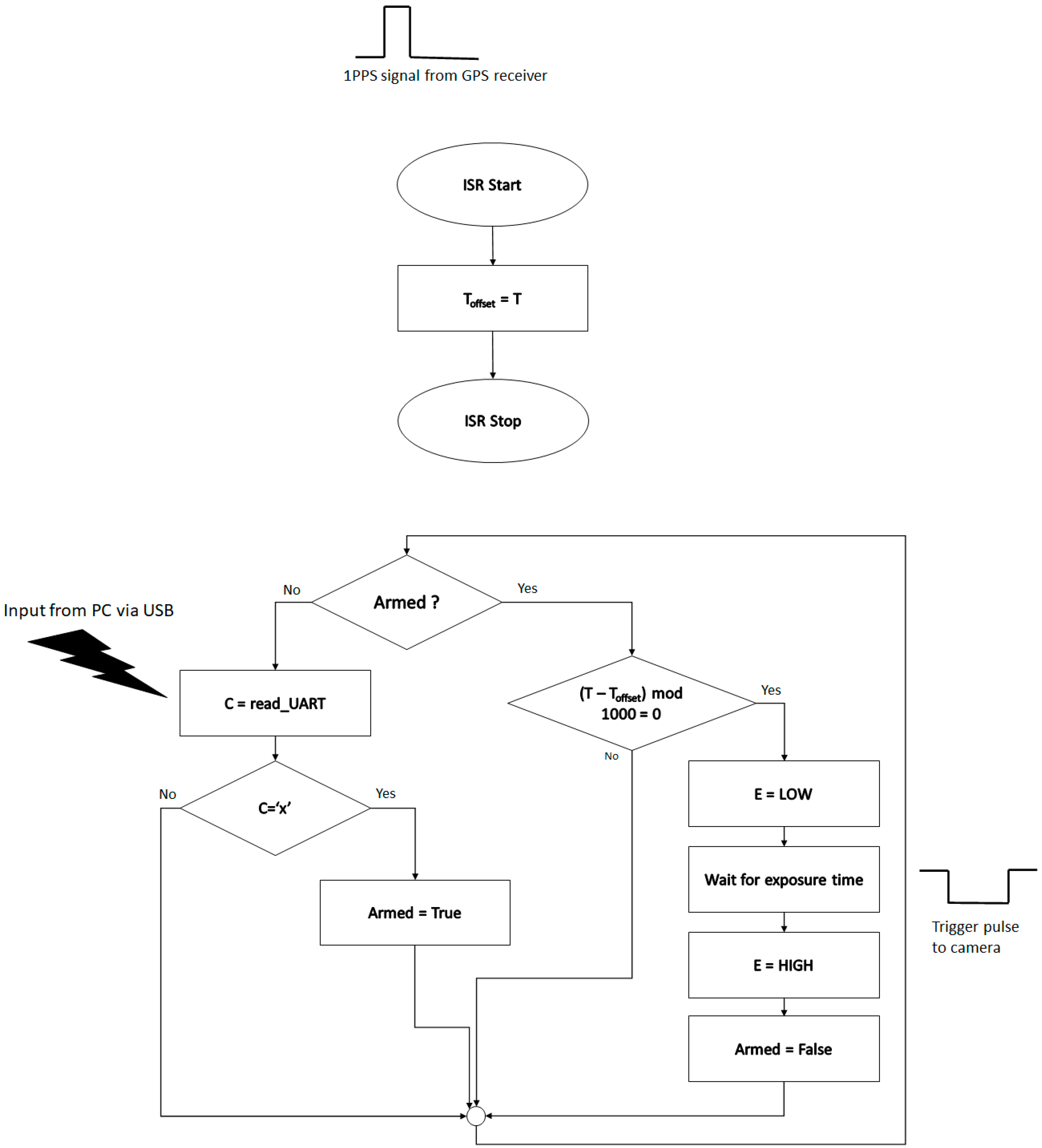
The algorithm running on the synchronization device for the triggering of one image is shown in Figure 3. The main idea is to use the 1pps signal from the GPS receiver to time the start of the exposure of the camera to the start of the UTC second. The 1pps signal is generated by the GPS receiver when the reception is good enough for accurate positioning and timing. Unfortunately, sometimes this signal can be temporarily lost, and thus relying on it for every frame can lead to lost frames in the acquisition sequence. For this reason, we have chosen the solution of using the internal timing mechanism of the microcontroller, but every time the 1pps signal is available, the internal time will be synchronized with the global time.
The program has a main loop, which processes inputs from the PC via the UART/USB interface. If the PC gives the trigger command (‘X’), the program goes into the ‘Armed’ mode and will trigger the camera at the next full second. The symbol T denotes the current microcontroller time, in milliseconds, and Toffset is the offset synchronized with the GPS 1pps signal. When the difference between them is an integer multiple of 1000, and the system is armed, the exposure digital signal (denoted as E) will be set to 0, opening the camera shutter. After the required exposure time has passed, the exposure signal is set to 1, and the shutter will be closed.
The 1pps signal from the GPS receiver is handled asynchronously using an interrupt service routine (ISR) attached to the external interrupt 0, which is configured to be triggered on the signal’s rising edge. The ISR will adjust the time offset Toffset to be equal to the current time T, thus bringing the internal time in sync with the global UTC time.
After the camera is triggered, the GPRMC string from the GPS receiver is read using a software serial interface and parsed to extract the time, and the name for the image file is created. This name is then sent to the PC. This process has not been depicted in Figure 3.
2.1.3. Software Architecture
The detection system has four main components, as shown in Figure 4. The acquisition component, which was described in the previous section, provides synchronized and timestamped images to the processing modules. The tracklet detection module uses the image sequence to detect differences between consecutive images, classifies these differences to extract streak candidates, and joins the streaks, if locally collinear, into tracklets. More details about this module will be presented in Section 2.2. The astrometric calibration module is based on the tools from astrometry.net, and because it is very computationally intensive, will use only one out of every 20 frames to compute the calibration information. The necessity of repeating the calibration periodically stems from the lack of sidereal tracking, which causes the star background to move. The angular results generation module takes the pixel coordinates of the tracklets and the calibration results and produces the final results, the tracklets in right ascension (RA) and declination (DEC) coordinates. The astrometric calibration and results generation module will be described in Section 2.3.
2.2. Tracklet Detection from Image Sequences
2.2.1. Extracting the Moving Features
The strategy for detecting the satellites from an image sequence takes advantage of their moving nature against the quasi-fixed starry background. If an accurate sidereal tracking system were used, the starry background can be assumed to be fixed. In a single frame, a satellite will cause a linear streak, as it moves during the camera exposure time. In consecutive frames, the streak will change its position, moving in a quasi-linear manner. These two properties lead to the basic strategy of finding different regions between consecutive frames, check to see whether these regions are elongated shapes that may be caused by a moving satellite, and then analyze subsequent frames to see whether the streaks detected in those frames are aligned on the same trajectory. This approach has been used before; as shown in [2,9], it can be implemented easily using basic image processing techniques and can process large images in real time, with robust results when the images are acquired under good observation conditions such as low light pollution, no clouds, and a fixed background, i.e., conditions that are usually available when the observation is carried out in an astronomical observatory. Our objective is to have a system that can work with light pollution from cities or the uneven background of the sunrise or the sunset, without star tracking to ensure a stationary background, and we aim to detect even the faint, short streaks, which are impossible to see with the naked eye. For these reasons, significant improvements had to be made to the basic streak detection approach.
The first problem to be solved is the unevenly lit background. This problem is especially relevant in the case of observing LEO satellites, as they are visible only near sunset or near sunrise, otherwise they are either in the Earth’s shadow or the sunlight is too powerful and renders them invisible. Unfortunately, these times are exactly the times the sky is unevenly lit. Figure 5 shows a full frame with uneven background light and the detail around a satellite streak (brightness and contrast are enhanced in the detail image, for visibility, but the enhancements are not used in the detection process).
The background light can be modeled as a parametric surface, whose parameters are estimated based on the observed data, as seen in [5]. However, this model can be limited if the sources of light pollution are multiple, such as city lights combined with the sunset/sunrise. In our experiments, we found that a median filter of a sufficiently large size can model the background light accurately, without the need for assumptions, as seen in Figure 6.
Formally, if we denote by It the image acquired at time t, and we compute the background light image Bt by median filtering, the dark background image Dt will be obtained by subtracting the background from the acquired image:
A detailed dark image is presented in Figure 7.
The sequence of dark background images Dt is then used for identifying the pixels belonging to moving regions. For each time stamp t, the image Dt is compared to the past image Dt−1, obtaining the movement image Mt.
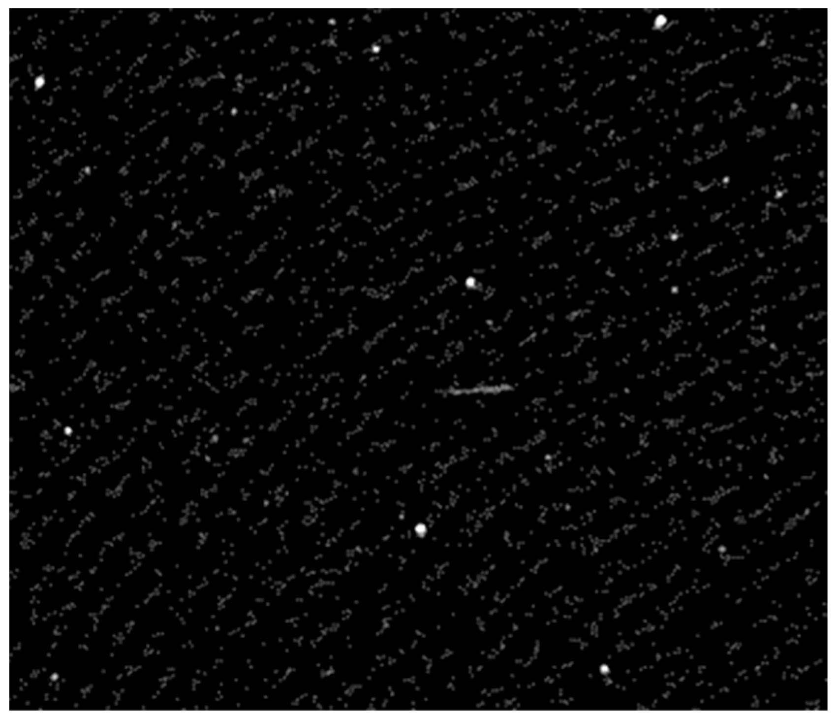
All subtractions shown in Equations (2) and (3) are performed using saturation, meaning that any pixel difference below 0 is set to 0. The movement image is then thresholded with a very low threshold (the threshold can be changed in the configuration file, usually we set it to Tthreshold = 2). In this way, any small variation of intensity is taken into consideration. The result for our detail window is seen (in negative) in Figure 8.
As we can see, many features, including parts of the stars, are present in the binary image. This is due mostly to the fact that we do not use a star tracking mount for the camera, to compensate for the Earth’s rotation. The satellite streaks will be extracted by further analyzing the size and shape of the binary objects.
2.2.2. Classifying Moving Features into Streak Candidates
The binary image is further processed by extracting the connected components, using the process of labeling. First, for each connected component, we compute the area or the number of pixels included in the object. This first property is used to filter out the binary objects that are too small to be taken into consideration. The area threshold, Athreshold, is a parameter of the system, and will be read from the configuration file. We have set this value to 15, experimentally.
The binary objects with the area below the threshold are discarded. For the remaining objects, the following geometric properties are computed:
- Center of mass (x0, y0),
- Major ellipse axis length (Lmajor),
- Minor ellipse axis length (Lminor),
- Eccentricity (e), computed from the axes’ lengths,
- Orientation angle (φ), computed from the points (x, y) belonging to the object S, and the center of mass.
The major axis length is compared to the threshold Lthreshold, read from the configuration file. A typical value is 30 pixels, but we can decrease this threshold for increased sensitivity for small streaks, which correspond to satellites further away. The eccentricity will also be compared to ethreshold, read from the configuration file. A value of 0.95 will identify the clear streaks, but for increased sensitivity in the presence of smaller streaks, this parameter can be decreased to 0.85 or even lower.
A summary of the conditions for an object to be accepted as a streak candidate:
- Area greater than Athreshold (15 pixels or more);
- Major ellipse axis length greater than Lthreshold (30 pixels typical, can be as low as 15 for increased sensitivity);
- Eccentricity greater than ethreshold (0.95 typical, but as low as 0.80 for increased sensitivity).
Together with Tthreshold used for binary image generation, these values are the configuration parameters of the algorithm.
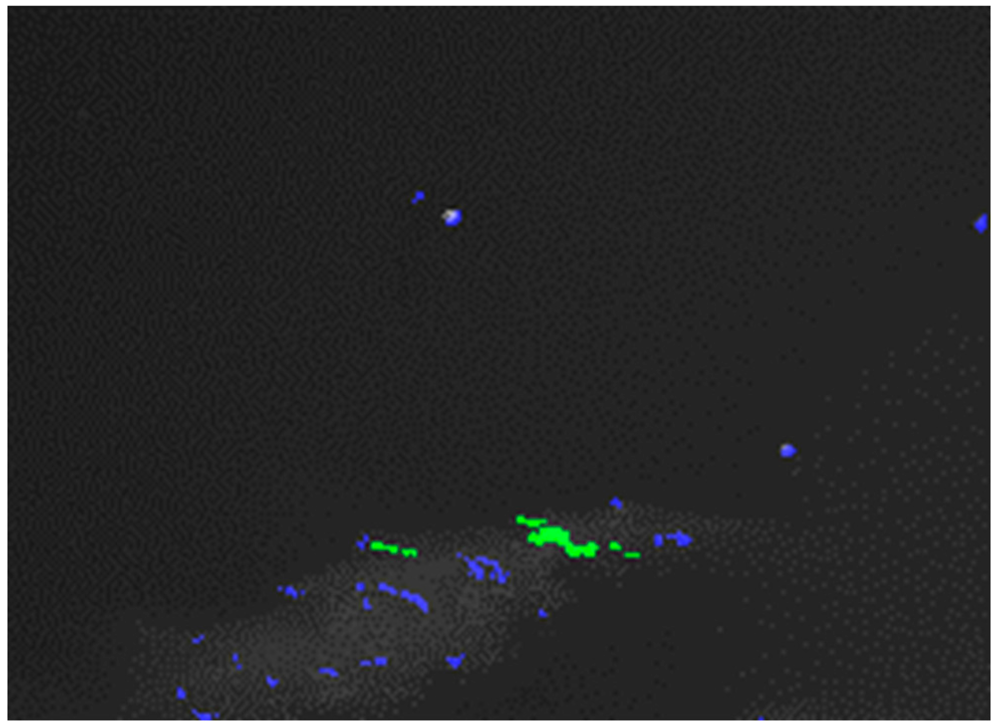
A result of the streak classification process is shown in Figure 9. The streak candidate has the pixels labeled with the color green, and the rest of the objects, which are caused by the relative motion of the stars in the background, are labeled blue. The contrast, brightness, and saturation are increased for better visualization.
The conditions for the streak candidate are not strict because the distance of a LEO from the observation site varies greatly, along with the perceived angular speed, and therefore the streak length can vary significantly. The variable brightness of the satellite also affects the thickness of the streak. Thus, strict criteria will lead to a lot of missed targets. However, our lax criteria will lead to a lot of false positives when other moving features are present in the image, such as clouds, as seen in Figure 10. In order to have the best of both worlds, high sensitivity and a low number of false positives, we validated the streaks by their trajectory.
2.2.3. Trajectory Analysis and Tracklet Formation
For every possible streak candidate, we computed three key points, which define the streak as a line segment (see Figure 11). The first point is the center of mass, already known, denoted as O, having the coordinates x0 and y0. The other two points are denoted as A and B, and their coordinates are computed by starting from the streak’s center and going along its orientation axis, progressively increasing the distance r from the center until the current point passes beyond the pixel set of the streak. The search is performed in both directions, and therefore the coordinates of the streak ends are computed as follows:
The distances from the center O, rA and rB, are usually equal, but they may differ when the streak has uneven illumination (for example, when the satellite is spinning fast).
The trajectories will be formed based on individual streaks detected in consecutive images. Having the two streaks defined by the three points O, A, and B, and O’, A′, B′, we can define two types of distances between them:
- The Euclidean distance between centroids, due to velocity, dV;
- The distances between one streak’s points and the line defined by the other streak, d(P, A, B), where P can be either the centroid of the new streak, O′, or one of the end points, A′ and B′.
The two types of distances are shown in Figure 11.
Figure 11.
Computing distances between two streaks.

A tracklet is a sequence of streaks that depict the same LEO object at different moments in time. A new tracklet is started when a new streak is detected, and this streak cannot be associated with an existing tracklet.
In our algorithm, a tracklet can have the following states:
State 0—empty tracklet.
State 1—a new streak has been detected, and a new tracklet has been initialized. In this state, the speed of the streak is not yet known, and neither is the orientation along the trajectory line. This state is depicted in Figure 12: the gray areas are the locations of the possible new streaks to be matched to this track. Even though we do not know the speed of the tracklet, we can assume that it is similar to the length of the streak, as the exposure time is equal to the time between frames (this is set explicitly in the acquisition program. A shorter or longer time between frames can be used, and the condition for the distance between streaks can be adjusted proportionally). Thus, we will impose an acceptable interval for the distance dV.
State 2—at least two streaks are associated with the tracklet, and therefore the speed and the orientation of the trajectory are known. In this state, the area allowed for the new detections is limited to the side pointed by the speed vector, as shown in Figure 13.
State 3—a state 2 tracker will eventually pass beyond the borders of the image, or no new streaks will be added to it for a significant number of frames. This state represents a “closed” tracklet, which will be delivered as output for the angular coordinates generation module.
The tracking (tracklet generation) algorithm:
- For each detected streak S
- For each active tracklet T (state 1 or 2)
- Predict the state of the tracklet based on the speed and the time stamp.
- Compute the centroid distance dV between the predicted centroid and the streak centroid, using equation (10). If the track is in state 1, assume the speed is equal to the streak length and make predictions on both sides.
- Compute the distances d(A′, A, B) and d(B′, A, B) between the extremities A′, B′ of the detected streak and the line defined by points A, B of the previous streak associated with the track using equation (11).
- If the distances dV, d(A′, A, B) and d(B′, A, B) are below a threshold, associate streak S with tracklet T.
- If T was in state 1, change the state to 2.
- If the prediction of the centroid falls outside of the image, change the state to 3, and output the tracklet results.
- If streak S remains unassociated with a tracklet, start a new tracklet from S, with state 1.
The process is illustrated step by step in Figure 14. When a new streak is detected, and it cannot be associated with an existing tracklet, a new tracklet is created as shown in Figure 14b. The tracklet has no clear orientation, only a linear direction. When a new streak is detected, it is associated with the new tracklet, as seen in Figure 14d. Now the tracklet has a clear orientation and will only associate with streaks that confirm to it, as seen in Figure 14f. The white circle represents the predicted centroid. When the tracklet is in state 1, the prediction is shown in the place of the first streak, but after the tracklet is in state 2, the prediction relies on the speed and orientation. When the prediction passes beyond the limits of the image, the tracklet is finished. The 2nd degree curve fit to the tracklet points is shown for illustration purposes only.
In Figure 14, at the bottom of the individual images, we can also see false streaks caused by clouds. While they will create new tracklets, these tracklets will usually not go beyond state 1, and therefore they will not be included in the results.
The result of the image processing algorithm is the tracklet file, containing the pixel coordinates and timestamps for all detected positions of a tracklet. An example of tracklet file contents:
          Track 73
          2021 11 24 3 14 4.080000 389.000000 433.000000
          2021 11 24 3 14 16.080000 608.000000 345.000000
          2021 11 24 3 14 23.080000 739.000000 294.000000
          2021 11 24 3 14 29.080000 863.000000 245.000000
          2021 11 24 3 14 35.080002 989.000000 197.000000
          2021 11 24 3 14 41.080002 1124.000000 148.000000
          2021 11 24 3 14 47.080002 1261.000000 98.000000
          2021 11 24 3 14 53.080002 1406.000000 47.000000
The first six columns contain the timestamp. The number that shows the second is not an integer because we added to the GPS time the camera shutter lag time, which for the Canon EOS 800D is 80 ms. The last two columns are the image x coordinate and the image y coordinate of the streak. The streak point identified by these coordinates is either point A or point B of the tracklet; the selection between them is based on the tracklet’s speed vector orientation. Our intention is to identify the first point of the streak corresponding to the satellite’s position in the image space at the start of the exposure time.
2.3. Astrometry and Angular Results Generation
2.3.1. Astrometric Calibration
The detection results are so far expressed in pixel coordinates, a tracklet being a sequence of (x, y) pixel coordinates associated with the acquisition timestamps for the corresponding frames. For the results to be useful from the SST perspective, they need to be expressed in astronomical, celestial angular coordinates. These coordinates are the right ascension (RA), similar to the geographical longitude, and the declination (DEC), similar to the geographical latitude. These coordinates can be further used to compute or update the orbit of the observed space object, a process which is beyond the scope of this paper.
The principle behind translation from pixels to RA/DEC coordinates is the use of background stars as reference markers. All stars are catalogued, and their RA/DEC coordinates are known, and therefore the process can be described as the task of identifying the stars in the image, creating a model of the coordinate mapping from the image pixels to the angular coordinates, and then mapping the detection points. While the process may sound simple, it involves a search through a very large parameter space, including the angular pixel size (the scale), which depends on the camera and the image sensor, the coordinates of the image center, which depend on the orientation of the camera/lens, the angle of the camera sensor with respect to the horizon, and the distortion (non-linearity) coefficients, which are not negligible when the observed field is as wide as in our case.
The freely available tools from Astrometry.net are designed to recognize the stars and generate the mapping between pixels and angular coordinates with minimum to no user input or prior knowledge about the acquisition conditions. The tools can be easily installed on any computer running a Unix-compatible operating system or even on Windows machines that use the Cygwin emulator. The tools work with .jpg images, such as in our case, but also with .FITS images acquired by professional astronomical cameras.
Figure 15 shows four types of calls to the field solver program of the Astrometry.net package, the program that automatically recognizes the stars in the input image and generates the pixels to RA/DEC angles mapping model. The first call is the generic, blind call, when no information about the acquisition conditions is available. This call is the simplest, can take a very long time to complete, but is useful when nothing is known about the lens and the camera. One of the most important pieces of information is the pixel size, which, after a successful first blind calibration can then be restricted to a narrow range, as long as the camera and lens are not changed. This is what is shown in the second call: as the initial calibration found a pixel size of about 92 arcseconds/pixel, we will limit the further calls to a lower limit (-L) of 85 and a higher limit (-H) of 95, specifying the unit or arcseconds per pixel (-u app). In this way, the calibration time is significantly shortened to about one minute or less.
Due to the fact that the observed field is 60 × 40 degrees wide, the default degree for the SIP (simple imaging polynomial) that models the nonlinear distortions of the plate calibration [27] is sometimes not accurate enough, especially for the peripheral areas of the image. We can instruct the calibration tool to use a higher degree polynomial, as seen in call number 3 (-t 7). The argument 7 is the degree of the distortion polynomial and was found by experiment. For a narrower field of view, this degree may be significantly lower than or to the left of the default value. In this way, the model will be more accurate, but the calibration time can be again increased.
Call number 4 shows how we can further decrease the processing time by using the past results to restrict the search field. The parameters RA and DEC in the call (--ra RA --dec DEC --radius 40) are the coordinates of the plate center obtained from the previous call in a sequence, forcing the next calibration to focus around the previous sky region instead of considering the whole sky. In this way, the processing time for each image can be reduced to about 10 s. This may seem as a major impediment to using the system for real-time detection, but one calibration can be used for multiple detections in subsequent frames.
Based on the four types of calls already described, and shown in Figure 15, the complete strategy for astrometric calibration is the following:
- Use blind call 1 for a new instrument, once, for establishing the angular size of the pixel.
- For an acquired image sequence, process every 1 in 20 frames:
- Use call 3 for the first processed frame to establish the first plate center by searching the whole sky;
- Use call 4 for the subsequent frames, restricting the search space around the previous found plate center;
- Store the calibration file along with its timestamp for converting the tracklets into RA/DEC coordinates.
A result of the automatic star recognition for an acquired image is shown in Figure 16.
2.3.2. Computing the Angular Coordinates of the Tracklets
If a calibration file is available, the astrometry.net tools can compute the relationship between image pixel coordinates and the world coordinates, by invoking the wcs-xy2rd command. The process is, however, complicated by the following challenges:
- The lack of sidereal tracking means that the sky configuration in the moment of calibration is not the same as the configuration for each observation point;
- Errors in calibration, due mostly to less-than-ideal conditions and to the wide field of view.
To overcome the first challenge, we have to take into consideration the time between the calibration and the observation. Denoting the time of the observation point i as ti, the time of the calibration c as tc, and the angular coordinates provided by wcs-xy2rd as RAc and DECc, the angular coordinates for the point i will be computed as:
In Equation (12), the times are expressed in hours, and the angles in degrees. The equation will compensate for the Earth’s rotation during the time difference, with a speed of 15 degrees for every sidereal hour. The term 1.0027379093 in Equation (12) is the conversion factor from UTC to sidereal time. The right ascension angle will be affected by this rotation, but the declination angle will not, as stated by Equation (13).
By compensating for the Earth’s rotation, we can use the calibration files at any time, as long as the time difference is not too high. For example, in 20 min, the sky will rotate by approximately 5 degrees, an amount which is almost 10% of our observation field, and therefore we have chosen not to use calibration files that have a higher time difference than 20 min from the observation time.
The second challenge is related to the errors in the astrometrical process. In order to overcome these errors, we compute, for each track, the angular coordinates using all available calibration files in the ±20 min range. While most of the results will be in agreement, there is a significant chance of outliers, as seen in Figure 17.
For each observation point i, and each of n usable calibration frames c (within the 40-min wide window, c), we have a list of right ascension values , and a list of declination values, The filtered, final result for the two angles will be provided by the median filter (Equations (14) and (15)), which eliminates the outliers and selects the middle value of a sorted sequence.
The final result will be written as a Track Data Message (.tdm) file [28]. The .tdm file for the tracklet shown in Figure 17 will have the following content:
          CREATION_DATE = 2022-01-17T09:50:0.000000
          ORIGINATOR = UTCN
          META_START
          COMMENT LONGITUDE 23.607456 EAST
          COMMENT LATITUDE 46.792990 NORTH
          COMMENT ALTITUDE 376.000000 M
          TIME_SYSTEM = UTC
          ANGLE_TYPE = RADEC
          REFERENCE_FRAME = EME2000
          META_STOP
          DATA_START
          ANGLE_1=2021-11-24T03:14:4.080000 224.247955
          ANGLE_2=2021-11-24T03:14:4.080000 51.636265
          ANGLE_1=2021-11-24T03:14:16.080000 216.112122
          ANGLE_2=2021-11-24T03:14:16.080000 49.333347
          ANGLE_1=2021-11-24T03:14:23.080000 211.565292
          ANGLE_2=2021-11-24T03:14:23.080000 47.648979
          ANGLE_1=2021-11-24T03:14:29.080000 207.471420
          ANGLE_2=2021-11-24T03:14:29.080000 45.897671
          ANGLE_1=2021-11-24T03:14:35.080002 203.605835
          ANGLE_2=2021-11-24T03:14:35.080002 43.953228
          ANGLE_1=2021-11-24T03:14:41.080002 199.806335
          ANGLE_2=2021-11-24T03:14:41.080002 41.710945
          ANGLE_1=2021-11-24T03:14:47.080002 196.226089
          ANGLE_2=2021-11-24T03:14:47.080002 39.337502
          ANGLE_1=2021-11-24T03:14:53.080002 192.780472
          ANGLE_2=2021-11-24T03:14:53.080002 36.729244
          DATA_STOP
3. Results
3.1. Testing Methodology
The detection results were tested against the known orbits of the satellites. The website space-track.org maintains up-to-date orbital information files for more than 20000 satellites and space debris, which can be freely downloaded. We developed a Matlab application that uses the SGP4 predictor [24] to generate angular coordinates for a given satellite’s orbital parameters, given observation timestamps, and the known geographical location of the observer. The application loads the result .tdm file, extracts the timestamps and the location, generates the predicted coordinates for each satellite based on its Two Line Element (TLE) data, and compares the results with the measured angles from the .tdm file. The process, for a given orbit and a given result file, is shown in Figure 18.
The predicted and the measured trajectories were compared using two error measurements, the Cross Track Error (cte) and the Along Track Error (ate). The Cross Track Error is the distance between corresponding line segments generated by the measurement and the prediction, and the Along Track Error is the error generated by the displacement of the detected point along the line segment (or along the trajectory). In practice, for every measurement point, we compute the distance to the closest predicted line segment, for computing the cte, and then the Euclidean distance to the predicted corresponding point. Using Pythagoras’ theorem, we obtain then the second side, which is the ate, as seen in Figure 19.
The cte and the ate are computed for every point of the tracklet. The cte and the ate errors for the whole tracklet are computed as the means of the individual point errors.
The validation application compares each result file of the acquired sequence with each satellite orbit downloaded from space-track.org. A match is declared if the cross-track error and along-track error are below some thresholds established as a function of sensor characteristics and object orbit type (e.g., eccentric orbits are subject to larger thresholds). For our sensor, a match is declared if the cross-track error is less than 1 degree and the along-track error is less than 10 degrees. These large thresholds are considered to cover cases of the re-entry objects, of which the orbits are strongly perturbed by the upper atmosphere conditions. If we exclude these objects, the thresholds could be considerably lower as can be seen from the results presented in Table 1 and Table 2.
3.2. Testing the Portable SST System
The complete portable SST system was tested in two locations in the city of Cluj-Napoca, Romania. The locations are in populated areas, with mostly houses less than three stories high, and the observations were made from balconies. The city lights and the light of sunset or sunrise were present, which created an uneven and fairly bright background.
Below we present the results for two sequences. The first sequence was captured with the camera facing south-west, where the LEO satellites are usually observable around sunset. A typical frame from the 2-h sequence is shown in Figure 20. Most of the detected satellites were not visible to the naked eyes.
In Figure 21, we can see several detected and recognized satellites. The system also detected satellite-like objects that were not recognized by the TLE-based prediction. Some of these objects were planes (the city of Cluj-Napoca also has an airport and the air traffic is significant), but some may also be satellites or space debris with outdated TLE data Unfortunately, for very faint objects, which can be either planes illuminated by the sun or space debris, we do not have any means of determining their nature. In Table 1, we also show the number of tracklets that we were not able to match with the TLE data, and by manual analysis of the image sequence, we identified that most of them were planes (11 out of 14), but there were still three tracklets with LEO characteristics.
The detected and recognized objects ranged from 600 to more than 1500 km from the observation point. The range was extracted from the orbit-based position prediction, as the detection system is not able to directly measure the range.
A summary of the sequence, including the errors, is shown in Table 1.
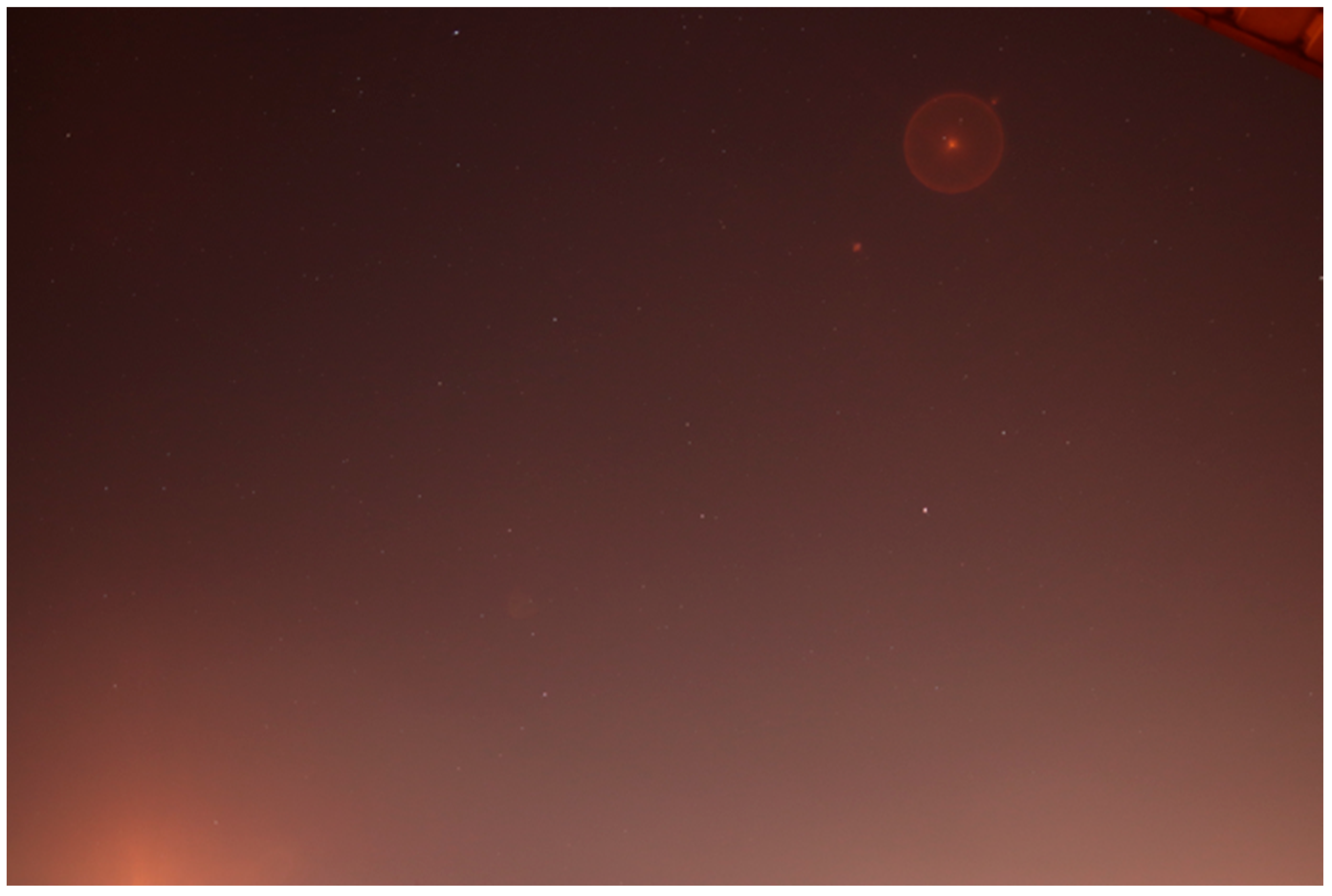
The second sequence was captured before sunrise, and the camera was oriented towards East. The location of the system, in this case, was more challenging, as the street lights were much closer and their effect was much more visible, even creating a lens flare, as seen in Figure 22, in the top right region. No satellites in this sequence could be seen by the naked eye or by directly looking at the images.
From this sequence, less than one hour long, the system detected 14 satellites, all recognized based on TLE orbital parameter prediction. The range, from prediction, was between 650 and 1300 km. A selection of recognized satellites, compared with their predicted trajectories, is shown in Figure 23.
A summary of the sequence, including the errors, is shown in Table 2.
From analysis of the errors, we observed that the cross-track errors were lower than the along-track errors: the average absolute error was equivalent to around 1 pixel, and the median cross-track error was nearly half a pixel, which means that the system is limited by the camera resolution and lens focal length and does not add errors through processing. The median errors were lower because they excluded the outliers that appeared when the satellite was first and last seen, and the streak was not completely included in the image.
The along-track error, for both sequences, was much higher. This is the error of locating the satellite along its trajectory at a specific moment in time, and therefore it is mostly caused by imperfections in the synchronization system. Due to the fact that the acquisitions were performed from balconies, the GPS did not have perfect reception, and the time synchronization was less than perfect.
3.3. Testing the Processing System with Precisely Timed Telescope Images
The software system can also act as an automatic processing tool for image sequences acquired with different instruments. We processed sequences provided by the Astronomical Observatory of Cluj-Napoca, acquired from the Feleacu observation site. For observing LEOs, the setup is based on an Orion ShortTube 80 telescope, with aperture of 80 mm and focal distance of 400 mm, mounted on a PlaneWave L600 equatorial mount, operating in star tracking mode. The images were acquired with an astronomical CCD camera operating in binning mode, the resulting FITS image size being 768 × 512 pixels. The field of view was 1.98 × 1.32 degrees, and the pixel angular size was 9.28 arcseconds. The time was precisely synchronized using a GNSS-based Synoptes device (https://www.spacetech.ro/en/synoptes/, last accessed on 11 April 2022).
All of the processing algorithms, from detection to .tdm file generation, were the same as for the wide-field instrument. There was no change in algorithm, not even in the algorithm settings (thresholds, etc.), with the sole exception of the range of the angular pixel size, which instead of 85 to 95 became much smaller, 8 to 10. A custom function for reading the FITS files and the metadata including the location and timestamp was added to the software tool.
A frame from a sequence acquired with the previously described setup is shown in Figure 24.
The ground truth was generated using the astrometrical reduction tool Astrometrica [29]. The accuracy comparison was based not on trajectory, but on the corresponding angular coordinates. The error statistics are shown in Table 3.
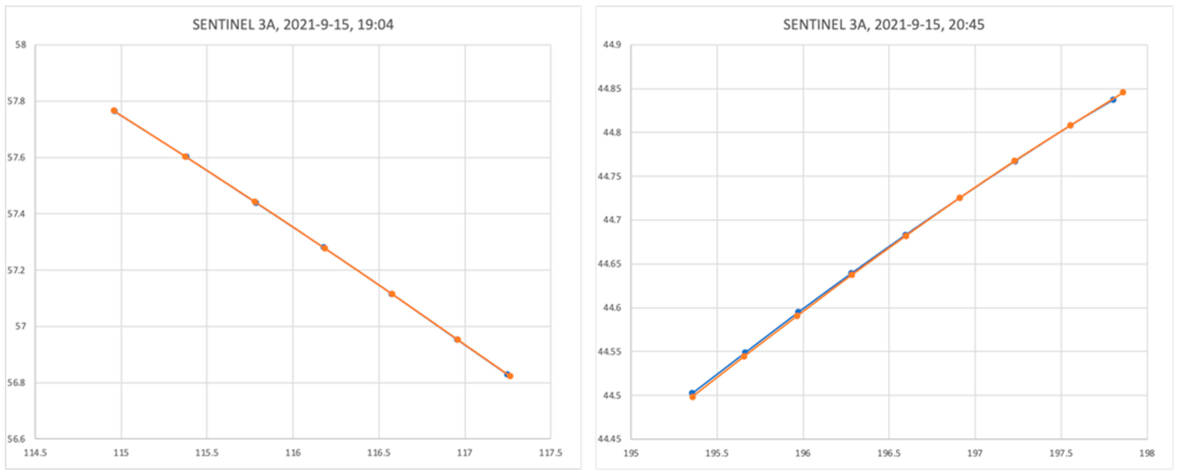
A selection of two trajectories, for the same satellite but different passes, is shown in Figure 25. We can see that the ground truth and the measured (by our system) position agree well, most errors being at the ends of the trajectories, where the streak is not completely included in the image.
The errors for the telescope sequence were less than one pixel, for both angles. This means that the software system is able to accurately measure the position of the target from the image sequences, and the overall accuracy is limited mostly by the precision of the time synchronization.
3.4. Execution Time
All of the processing steps, detection, calibration, and results generation were performed on the same PC used for triggering the camera, the 13-inch 2020 MacBook Pro, equipped with the Apple M1 processor and 16 GB of RAM. The typical execution times for a 1.5-h sequence are:
- Image processing (detection): 5 min
- Astrometric calibration: 20 min
- Results generation: 15 min
Therefore, the system is able to provide the .tdm results in about 40 min from the completion of the acquisition.
4. Discussion
The errors resulting from testing in a real environment of our portable SST system “SST Anywhere” are in the range of a few pixels in both along-track and cross-track directions. The cross-track error median values were around 1 pixel, which was as expected. Larger values were obtained for along-track errors, which are due to synchronization errors (lack of GPS signal). These synchronization errors also manifested in the cross-track errors, but their effects were less obvious than the effects for along-track errors.
The total number of objects detected and validated in the two experimental testing runs are in line with the expected detections corresponding to the aperture, FOV of our system, and the specific urban sky background conditions.
When we tested only the processing system using precisely timed telescope satellite image sequences in the astronomical observatory environment, the median errors in both RA and DEC were below 1 pixel compared with the standard processing system “Astrometrica”. Some differences in the residuals remained. Fine-tuning and analysis of the astronomical corrections considered/omitted in the compared processing software are further needed.
The total processing time for a typical 1.5-h observation sequence, obtained with our portable SST system, is about 40 min. This value is less than half of the rotation period or when applicable, the interval between two consecutive transits of the same LEO object. This observation is important if we want to use our portable system for refinement of an Initial Orbit Determination for an object or to further incorporate our system in a “Stare and Chase” architecture.
A comparison of our system with a similar large FOV system for SST mentioned in Section 1.1 is provided in Table 4.
We included in the comparison four LEO optical surveillance systems (LEOOS) and one of the “classical” LEO optical tracking systems: TAROT. LEOOS have the advantage of a larger FOV and do not require a mount, but are less sensitive and precise compared with TAROT or other comparable LEO optical tracking systems.
Our system is in line with the other three LEOOS regarding the optics: it uses a COTS photographical objective but a DSLR camera body instead of CCD/CMOS astronomical cameras used in the other three LEOOS. This option for our system has some advantages in terms of portability, pixel dimension, image file formats, and most notably, the estimated costs. At the same time, the use of the APS-C CMOS sensor comes with disadvantages regarding the sensor area and quantum efficiency. However, the resulting FOV is the second largest in the analyzed LEOOS.
The ultimate comparison characteristics between LEOOS should be the along-track and cross-track errors. These errors are influenced by the sensor performances, algorithms for LEO object detection, astrometric reduction, and the precision of orbital elements for LEO objects used for calculation of reference orbits. As a result, a suitable comparison between LEOOS is difficult to make. The error estimations for our system are comparable with [14], presenting a similar disparity between ATE and CTE.
The estimated costs for all analyzed systems were made taking into account the optics, the optoelectronic sensor/camera, and time synchronization devices with actual prices, excluding processing hardware and software and auxiliary costs for automatization, which are difficult to establish and compare. From this perspective, our system is the cheapest.
All of the analyzed systems are either a prototype or part of a multisensor or network array. Site astronomical conditions play an important role, as well as geographical distribution in the network cases. Our sensor was tested in a less than ideal astronomical environment, and part of the poorer performance was due to the poor visibility conditions.
5. Conclusions
We have presented a complete and portable system for image acquisition, image processing, and astrometric reduction, which can be easily set up anywhere to survey a large portion of the sky for low-Earth orbit objects. While not quite real time, the system is able to produce angular results in less than one hour after the sequence is acquired, and the accuracy is limited only by the resolution of the image sensor and the precision of the time synchronization. The system can also be used to automatically process sequences acquired from other sources, in .jpg or .fits format, with wide or narrow fields of view.
There are two problems that need to be addressed in future work: one is the problem of false tracklets generated by passing planes, which can be solved by further analysis of the intensity profile of the streak and of its neighboring pixels (the planes have position lights that cause flashes as they move), and the other is the introduction of a real-time operation mode. The main challenge of real-time operation is the lack of multiple images for calibration, which will cause the loss of accuracy of the results, and some kind of iterative refinement of the results will need to be carried out as the data become available. However, a real-time operation in the wide field, even with diminished precision, can be used to automatically target a narrow-field instrument, which can greatly improve the accuracy of the final results.
Author Contributions
Conceptualization, R.G.D.; methodology, R.G.D. and R.I.; software, R.G.D., R.I. and M.P.M.; validation, R.G.D., A.R. and V.T.; writing—original draft preparation, R.G.D.; writing—review and editing, A.R. and V.T.; project administration, R.G.D. All authors have read and agreed to the published version of the manuscript.
Funding
The research was supported by a grant from the Ministry of Research and Innovation, CNCS–UEFISCDI, project number PN-III-P2-2.1-PED-2019-4819, within PNCDI III, and also by a grant from the Ministry of Research, Innovation and Digitization, CNCS/CCDI–UEFISCDI, project number PN-III-P2-2.1-SOL-2021-2-0192, within PNCDI III.
Data Availability Statement
The complete sequences used for the statistics in Table 1 and Table 2, including the original image files, the result TDM files, and the satellite matching reports, can be downloaded from https://drive.google.com/drive/folders/1bNtM00Qx3tclZYBBZSAt50B7Hz9XRGPq?usp=sharing (last accessed on 11 April 2022).
Conflicts of Interest
The authors declare no conflict of interest.
References
- European Space Agency. Space Safety. Available online: https://www.esa.int/Our_Activities/Space_Safety/Space_Surveillance_and_Tracking_-_SST_Segment (accessed on 9 February 2022).
- Stoveken, E.; Schildknecht, T. Algorithms for the optical detection of space debris objects. In Proceedings of the 4th European Conference on Space Debris, Darmstadt, Germany, 18–20 April 2005; pp. 637–640. [Google Scholar]
- Maksim, S. A comparison between a non-linear, poisson-based statistical detector and a linear, gaussian statistical detector for detecting dim satellites. In Proceedings of the Advanced Maui Optical and Space Surveillance Technologies Conference, Maui, HI, USA, 11–14 September 2012; p. 44. [Google Scholar]
- Sara, R.; Cvrcek, V. Faint streak detection with certificate by adaptive multi-level bayesian inference. In Proceedings of the European Conference on Space Debris, Darmstadt, Germany, 17–21 April 2017. [Google Scholar]
- Levesque, M.P.; Buteau, S. Image Processing Technique for Automatic Detection of Satellite Streaks; Technical Report; Defence Research and Development: Valcartier, QC, Canada, 2007. [Google Scholar]
- Diprima, F.; Santoni, F.; Piergentili, F.; Fortunato, V.; Abbattista, C.; Amoruso, L. Efficient and automatic image reduction framework for space debris detection based on gpu technology. Acta Astronaut. 2018, 145, 332–341. [Google Scholar] [CrossRef]
- Ciurte, A.; Danescu, R. Automatic detection of MEO satellite streaks from single long exposure astronomic images. In Proceedings of the International Conference on Computer Vision Theory and Applications (VISAPP), Lisbon, Portugal, 5–8 January 2014. [Google Scholar]
- Hickson, P. A fast algorithm for the detection of faint orbital debris tracks in optical images. Adv. Space Res. 2018, 62, 3078–3085. [Google Scholar] [CrossRef] [Green Version]
- Danescu, R.; Oniga, F.; Turcu, V.; Cristea, O. Long baseline stereo-vision for automatic detection and ranging of moving objects in the night sky. Sensors 2012, 12, 12940–12963. [Google Scholar] [CrossRef] [PubMed] [Green Version]
- Do, H.N.; Chin, T.J.; Moretti, N.; Jah, M.K.; Tetlow, M. Robust foreground segmentation and image registration for optical detection of geo objects. Adv. Space Res. 2019, 64, 733–746. [Google Scholar] [CrossRef]
- Martin, L. Space Fence. Available online: https://www.lockheedmartin.com/en-us/products/space-fence.html (accessed on 15 February 2022).
- Park, J.H.; Yim, H.S.; Choi, Y.J.; Jo, J.H.; Moon, H.K.; Park, Y.S.; Roh, D.G.; Cho, S.; Choi, E.J.; Kim, M.J.; et al. OWL-Net: Global Network of Robotic Telescopes for Satellites Observation. Adv. Space Res. 2018, 62, 152–163. [Google Scholar] [CrossRef]
- Boër, M.; Klotz, A.; Laugier, R.; Richard, P.; Dolado Perez, J.-C.; Lapasset, L.; Verzeni, A.; Théron, S.; Coward, D.; Kennewell, J.A. TAROT: A network for Space Surveillance and Tracking operations. In Proceedings of the 7th European Conference on Space Debris, Darmstadt, Germany, 17–21 April 2017. [Google Scholar]
- Hasenohr, T. Initial Detection and Tracking of Objects in Low Earth Orbit. Available online: https://elib.dlr.de/110661/1/Initial%20Detection%20and%20Tracking%20of%20Objects%20in%20Low%20Earth%20Orbit.pdf (accessed on 9 February 2022).
- Kaminski, K.; Zołnowski, M.; Wnuk, E.; Golebiewska, J.; Kruzynski, M.; Kaminska, M.K.; Gedek, M. Low Leo Optical Tracking Observations With Small Telescopes. In Proceedings of the 1st NEO and Debris Detection Conference, Darmstadt, Germany, 22–24 January 2019. [Google Scholar]
- Aume, C.; Andrews, K.; Pal, S.; James, A.; Seth, A.; Mukhopadhyay, S. TrackInk: An IoT-Enabled Real-Time Object Tracking System in Space. Sensors 2022, 22, 608. [Google Scholar] [CrossRef] [PubMed]
- Wijnen, T.P.G.; Stuik, R.; Redenhuis, M.; Langbroek, M.; Wijnja, P. Using All-Sky optical observations for automated orbit determination and prediction for satellites in Low Earth Orbit. In Proceedings of the 1st NEO and Debris Detection Conference, Darmstadt, Germany, 22–24 January 2019. [Google Scholar]
- Talens, G.J.J.; Spronck, J.F.P.; Lesage, A.-L.; Otten, G.P.P.L.; Stuik, R.; Pollacco, D.; Snellen, I.A.G. The Multi-site Al-Sky CAmeRA (MASCARA). Finding transiting exoplanets around bright (mV <8) stars. Astron. Astrophys. 2017, 601, A11. [Google Scholar]
- Stuik, R.; Bailey, J.I., III; Dorval, P.; Talens, G.J.J.; Laginja, I.; Mellon, S.N.; Lomberg, B.B.D.; Crawford, S.M.; Ireland, M.J.; Mamajek, E.E.; et al. bRing: An observatory dedicated to monitoring the β Pictoris b Hill sphere transit. Astron. Astrophys. 2017, 607, A45. [Google Scholar] [CrossRef] [Green Version]
- Kerr, E.; López, B.D.C.; Maric, N.; Torres, J.N.; Falco, G.; Sánchez Ortiz, N.; Dorn, C.; Eves, S. Design and prototyping of a low-cost LEO optical surveillance sensor. In Proceedings of the 8th European Conference on Space Debris, Darmstadt, Germany, 20–23 April 2021. [Google Scholar]
- López, B.D.C.; Kerr, E.; Torres, J.N.; Dorn, C.; Eves, S. Developing and Testing of aNovel Low-Cpsost LEO Optical Surveillance Sensor. In Proceedings of the Advanced Maui Optical and Surveillance Technologies Conference (AMOS), Maui, HI, USA, 14–17 September 2021. [Google Scholar]
- Utzmann, J.; Dimitrova Vesselinova, M.G.; Fernandez, O.R. Airbus Robotic Telescope. In Proceedings of the 1st NEO and Debris Detection Conference, Darmstadt, Germany, 22–24 January 2019. [Google Scholar]
- Lang, D.; Hogg, D.W.; Mierle, K.; Blanton, M.; Roweis, S. Astrometry.net: Blind astrometric calibration of arbitrary astronomical images. Astron. J. 2010, 139, 1782–1800. [Google Scholar] [CrossRef] [Green Version]
- Roweis, S.; Lang, D.; Mierle, D.; Hogg, D.; Blanton, M. Making the Sky Searchable: Fast Geometric Hashing for Automated Astrometry. Available online: https://cosmo.nyu.edu/hogg/research/2006/09/28/astrometry_google.pdf (accessed on 3 March 2022).
- Høg, E.; Fabricius, C.; Makarov, V.V.; Urban, S.; Corbin, T.; Wycoff, G.; Bastian, U.; Schwekendiek, P.; Wicenec, A. The Tycho-2 catalogue of the 2.5 million brightest stars. Astron. Astrophys. 2000, 355, L27–L30. [Google Scholar]
- Vallado, D. Fundamentals of Astrodynamics and Applications, 4th ed.; Microcosm Press: Cleveland, OH, USA, 2013. [Google Scholar]
- Shupe, D.L.; Moshir, M.; Li, J.; Makovoz, D.; Narron, R.; Hook, R.N. The SIP Convention for Representing Distortion in FITS Image Headers. In Proceedings of the Astronomical Data Analysis Software and Systems XIV—ASP Conference Series, Pasadena, CA, USA, 14–16 November 2005. [Google Scholar]
- The Consultative Committee for Space Data Systems Tracking Data Message—RECOMMENDED STANDARD CCSDS 503.0-B-1. Available online: https://public.ccsds.org/Pubs/503x0b1s.pdf (accessed on 9 February 2022).
- Raab, H. Astrometrica—Shareware for Research Grade CCD Astrometry. Available online: http://www.astrometrica.at/ (accessed on 9 February 2022).
- Klotz, A.; Boër, M.; Eysseric, J.; Damerdji, Y.; Laas-Bourez, M.; Pollas, C.; Vachier, F. Robotic Observations of the Sky with TAROT: 2004–2007. Publ. Astron. Soc. Pac. 2008, 120, 1298–1306. [Google Scholar] [CrossRef] [Green Version]
Figure 2.
One assembled portable SST system.

Figure 3.
The triggering algorithm of the synchronization interface.

Figure 4.
The software components of the LEO tracklet detection system.

Figure 5.
Captured image, converted to grayscale, showing an unevenly lit background. On the right side a detail of the full image is shown, with the faint satellite streak.
Figure 5.
Captured image, converted to grayscale, showing an unevenly lit background. On the right side a detail of the full image is shown, with the faint satellite streak.

Figure 6.
The background light for the image in Figure 5, extracted by median filtering in a neighborhood of 55 pixels radius.
Figure 6.
The background light for the image in Figure 5, extracted by median filtering in a neighborhood of 55 pixels radius.

Figure 7.
Detailed region after background subtraction.

Figure 8.
Binary image, following thresholding of the movement image.

Figure 9.
Objects classification: the streak candidate is shown in green, and the other large area objects in blue.
Figure 9.
Objects classification: the streak candidate is shown in green, and the other large area objects in blue.

Figure 10.
False streaks caused by clouds. The green areas are possible streaks, while the blue areas show movement but they are rejected by the shape criteria.
Figure 10.
False streaks caused by clouds. The green areas are possible streaks, while the blue areas show movement but they are rejected by the shape criteria.

Figure 12.
A tracklet in state 1: a single streak is detected, and the following streak can be on either side.
Figure 12.
A tracklet in state 1: a single streak is detected, and the following streak can be on either side.

Figure 13.
A tracklet in state 2: the tracklet now has speed and orientation, and new detections can only match in one direction.
Figure 13.
A tracklet in state 2: the tracklet now has speed and orientation, and new detections can only match in one direction.

Figure 14.
The evolution of a tracklet: (a,b) a new streak is detected, and a tracklet is formed; (c,d) the tracklet, in state 1, will be associated with a newly detected streak, and its state will be changed to 2; (e,f) the tracklet is in state 2 and associates with a new streak that matches the prediction of speed and orientation; (g,h) a completed tracklet, in state 3.

Figure 15.
Using the astrometry engine for obtaining the calibration between pixels and angular coordinates.
Figure 15.
Using the astrometry engine for obtaining the calibration between pixels and angular coordinates.

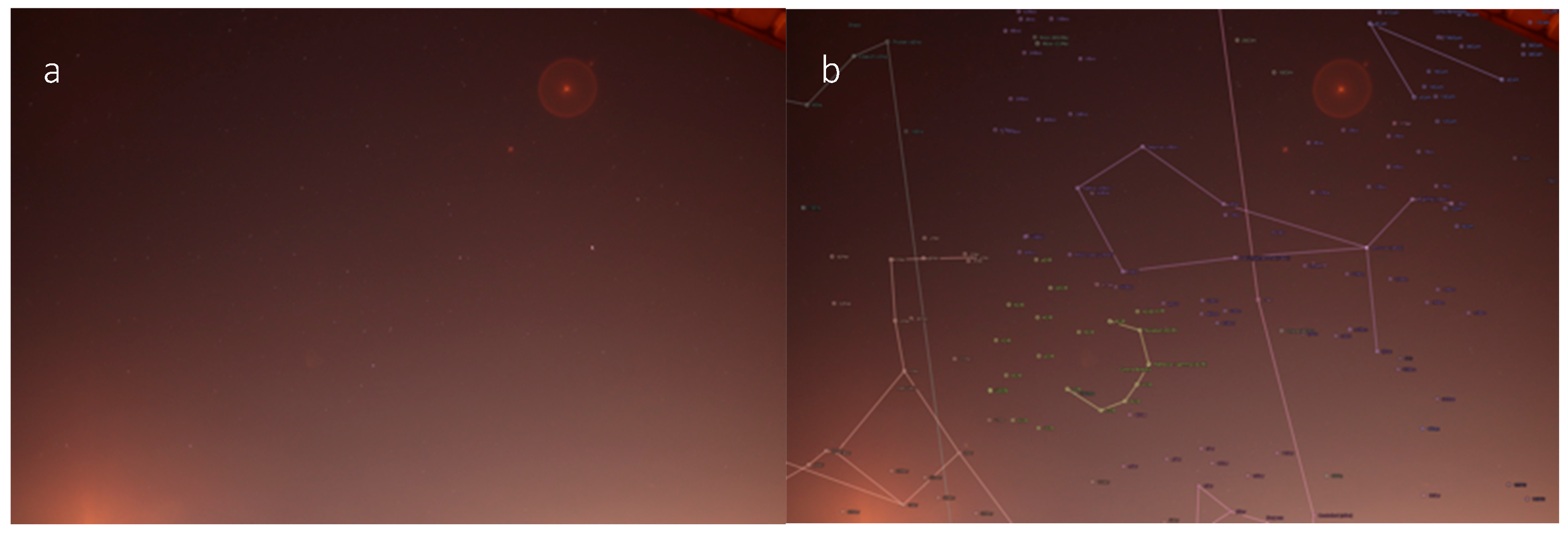
Figure 16.
Astrometric calibration results: (a) input image, (b) recognized constellations.

Figure 17.
Angular coordinates for a single tracklet, computed with different calibration files. While most of the results are in agreement, outliers are present.
Figure 17.
Angular coordinates for a single tracklet, computed with different calibration files. While most of the results are in agreement, outliers are present.

Figure 18.
The TLE-based validation methodology.

Figure 19.
The cross-track error (cte) and the along-track error (ate) between two trajectories.

Figure 20.
A frame from a sequence captured in Cluj-Napoca, at sunset, facing south-west. An LEO streak is highlighted by the red circle.
Figure 20.
A frame from a sequence captured in Cluj-Napoca, at sunset, facing south-west. An LEO streak is highlighted by the red circle.

Figure 21.
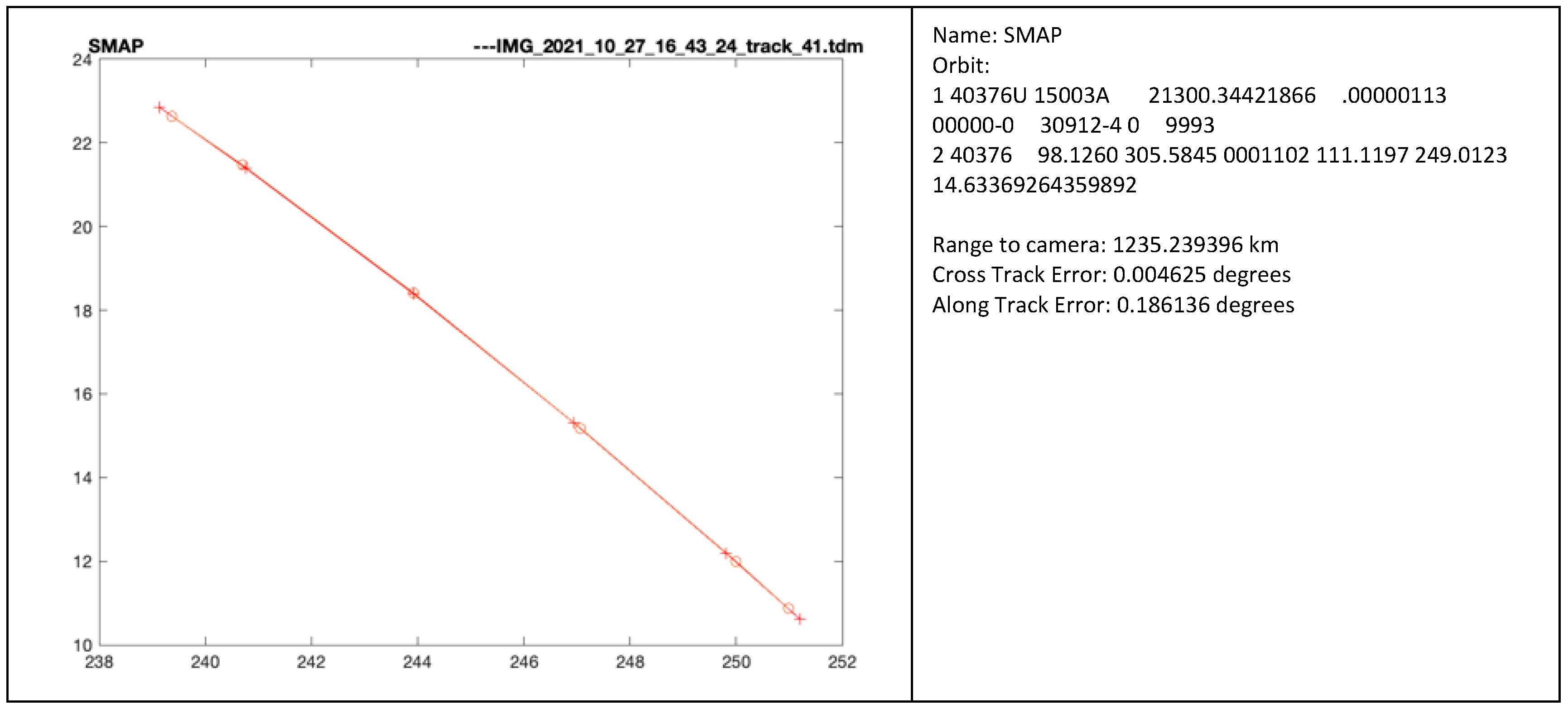
Selection of detected satellites (SW sequence). In the left column we can see the trajectory comparison between the prediction (marked with X) and the measurement (marked with O), and in the right column we see the satellite name, the orbital parameters, and the errors. Frame from a sequence captured in Cluj-Napoca, at sunset, facing south-west.
Figure 21.
Selection of detected satellites (SW sequence). In the left column we can see the trajectory comparison between the prediction (marked with X) and the measurement (marked with O), and in the right column we see the satellite name, the orbital parameters, and the errors. Frame from a sequence captured in Cluj-Napoca, at sunset, facing south-west.


Figure 22.
A frame from a sequence captured in Cluj-Napoca, before sunrise, facing East.

Figure 23.
Selection of detected satellites (East sequence). In the left column we can see the trajectory comparison between the prediction (marked with X) and the measurement (marked with O), and in the right column we see the satellite name, the orbital parameters, and the errors.
Figure 23.
Selection of detected satellites (East sequence). In the left column we can see the trajectory comparison between the prediction (marked with X) and the measurement (marked with O), and in the right column we see the satellite name, the orbital parameters, and the errors.


Figure 24.
An LEO photographed through the Orion ShortTube 80 telescope.

Figure 25.
Two passes of the Sentinel 3A satellite. The ground truth is shown in blue, and the measurement in orange.
Figure 25.
Two passes of the Sentinel 3A satellite. The ground truth is shown in blue, and the measurement in orange.


Table 1.
Error statistics for the SW sequence.
| Orientation | South-West |
| Duration | 16:25:23–18:55:18 |
| Date | 27 October 2021 |
| Mean Cross Track Error (arcsec) | 215.1380 |
| Mean Cross Track Error (pixels) | 2.3384 |
| Median Cross Track Error (arcsec) | 100.5876 |
| Median Cross Track Error (pixels) | 1.0933 |
| Mean Along Track Error (arcsec) | 574.7124 |
| Mean Along Track Error (pixels) | 6.2468 |
| Median Along Track Error (arcsec) | 413.7912 |
| Median Along Track Error (pixels) | 4.4977 |
| Number of matched detected objects | 25 |
| Number of non-matched detections | 14 |
| Number of planes (manual analysis) | 11 |
| Number of possible non-matched LEOs | 3 |
Table 2.
Error statistics for the East sequence.
| Orientation | East |
| Duration | 03:11:04–03:55:48 |
| Date | 24 November 2021 |
| Mean Cross Track Error (arcsec) | 108.3147 |
| Mean Cross Track Error (pixels) | 1.1773 |
| Median Cross Track Error (arcsec) | 48.1284 |
| Median Cross Track Error (pixels) | 0.5231 |
| Mean Along Track Error (arcsec) | 1008.1054 |
| Mean Along Track Error (pixels) | 10.9576 |
| Median Along Track Error (arcsec) | 435.0348 |
| Median Along Track Error (pixels) | 4.7286 |
| Number of matched detected objects | 14 |
| Number of non-matched detections | 0 |
| Number of planes (manual analysis) | 0 |
| Number of possible non-matched LEOs | 0 |
Table 3.
Error statistics for the telescope sequence.
| Duration | 19:08:58–20:07:10 |
| Date | 15 September 2021 |
| Mean RA Error (arcsec) | 12.8055 |
| Mean RA Error (pixels) | 1.3799 |
| Median RA Error (arcsec) | 8.5610 |
| Median RA Error (pixels) | 0.9225 |
| Mean DEC Error (arcsec) | 9.1181 |
| Mean DEC Error (pixels) | 0.9825 |
| Median DEC Error (arcsec) | 6.1644 |
| Median DEC Error (pixels) | 0.6642 |
| Number of detected objects | 10 |
Table 4.
Comparison of the main characteristics of similar LEO optical surveillance sensors.
| Reference | Hasenohr [14] | Wijnen et al. [17] | Kerr et al. [20] | Boër et al. [13] | Present Work | |
| Name & Location | DLR, Uhlandshöhe, Stuttgart, Germany | bRing, Sunderland, South Africa | LCLEOSEN, Deimos Sky Survey, Spain | TAROT-TRE, Reunion Island, France | SST Anywhere, Cluj-Napoca, Romania | |
| latitude | deg | 48.7824 N | 32.3812 S | 38.54362 | 24.1833 S | 46.75804 N |
| longitude | deg | 9.1964 E | 20.8102 E | 4.40844 W | 55.4166 E | 23.58809 E |
| Elevation | m | 399 | 1798 | 1065 | 1000 | 410 |
| Working mode | Surveillance | Surveillance | Surveillance | Tracking | Surveillance | |
| Telescope/lens | Canon EF 135 mm f/2 L USM | Canon 24 mm f/1.4 USML II | Canon 85 mm f/1.4 | Takahashi/CNRS Newton hyperbolic | Sigma EX DG RF 20 mm F1.8 | |
| Aperture | mm | 67.5 | 17 | 60.7 | 180 | 11.11 |
| Focal length | mm | 135 | 24 | 85 | 576 | 20 |
| Optoelectronic sensor | CCD (FLI Proline PL16803) | CCD (FLI Microline 11002 | CMOS (FLI Kepler KL4040) | CCD (FLI Proline PL16803) | CMOS (Canon 24.2 MP APS-C CMOS) | |
| Max. Quantum Efficiency | % | 60 | 50 | 68 | 50 | 43 |
| HxV dimensions | pixels | 4096 × 4096 | 4008 × 2672 | 2048 × 2048 | 4096 × 4096 | 2400 × 1600 |
| Pixel dimension (including binning) | microns | 9 × 9 | 9 × 9 | 18 × 18 | 9 × 9 | 9.37 × 9.37 |
| Resolution/pixel | arcsec | 13.75 | 66.5 | 44.8 | 3.22 | 92.0 |
| Field of View (H× V) | deg × deg | 15.27 × 15.27 | 74 × 53 | 25.4 × 25.4 | 3.66 × 3.66 | 61.3 × 40.9 |
| Exposure time | s | 1 | 6.4 | 0.1 | 10 | 5 |
| Measurement rate | s | 13 | 12.8 | 3 | 15 | 10 |
| Limiting Magnitude (Texp) | mag | No information available | 10 (6.4) | 9 (0.1 sec) | 16 (60 sec) | 10.5 (5 sec) |
| Along track error | arcsec | 874 *recapture | >66.5 | 2 | 0.8 | 414 (TLE) |
| Cross track error | arcsec | 692 *recapture | >66.5 | 2 | 0.8 | 101 (TLE) |
| Mount type & speed | No | No | No | Equatorial; 60 deg/s | No | |
| Dome/enclosure | Clamshell dome | Custom Fixed enclosure | Clamshell dome | Custom automatic enclosure | No | |
| Time synchronization | Microcontroller + GPS | Galleon NTS-4000-GPS-R Server | Chronostamper + GPS | Symmetricon GPS timer board [30] | Microcontroller + GPS | |
| Image files | FITS | FITS | FITS | FITS | JPG, RAW, FITS | |
| Processing time | min | 0.12 (recapture) | No information available | 162 (for 3-h observations) | No information available | 40 (for 1.5-h observations) |
| Estimated Costs (without enclosure and processing) | Euros | 16,100 | 18,100 | 16,700 | 33,300 | 1700 |
| Observations | Prototype for 5–9 multisensors | Part of a multisensor 2–5 elements | Prototype for 28 multisensors | Part of a network of four telescopes | Two identical systems were realized |
Publisher’s Note: MDPI stays neutral with regard to jurisdictional claims in published maps and institutional affiliations. |
© 2022 by the authors. Licensee MDPI, Basel, Switzerland. This article is an open access article distributed under the terms and conditions of the Creative Commons Attribution (CC BY) license (https://creativecommons.org/licenses/by/4.0/).
Share and Cite
MDPI and ACS Style
Danescu, R.G.; Itu, R.; Muresan, M.P.; Rednic, A.; Turcu, V. SST Anywhere—A Portable Solution for Wide Field Low Earth Orbit Surveillance. Remote Sens. 2022, 14, 1905. https://0-doi-org.brum.beds.ac.uk/10.3390/rs14081905
AMA Style
Danescu RG, Itu R, Muresan MP, Rednic A, Turcu V. SST Anywhere—A Portable Solution for Wide Field Low Earth Orbit Surveillance. Remote Sensing. 2022; 14(8):1905. https://0-doi-org.brum.beds.ac.uk/10.3390/rs14081905
Chicago/Turabian StyleDanescu, Radu Gabriel, Razvan Itu, Mircea Paul Muresan, Ana Rednic, and Vlad Turcu. 2022. "SST Anywhere—A Portable Solution for Wide Field Low Earth Orbit Surveillance" Remote Sensing 14, no. 8: 1905. https://0-doi-org.brum.beds.ac.uk/10.3390/rs14081905
Note that from the first issue of 2016, this journal uses article numbers instead of page numbers. See further details here.