
Hyperspectral Image Classification Based on Spectral Multiscale Convolutional Neural Network


1
College of Communication and Electronic Engineering, Qiqihar University, Qiqihar 161000, China
2
College of Information and Communication Engineering, Dalian Nationalities University, Dalian 116000, China
*
Author to whom correspondence should be addressed.
Remote Sens. 2022, 14(8), 1951; https://0-doi-org.brum.beds.ac.uk/10.3390/rs14081951
Submission received: 19 March 2022
/
Revised: 15 April 2022
/
Accepted: 16 April 2022
/
Published: 18 April 2022
(This article belongs to the Special Issue Recent Advances in Processing Mixed Pixels for Hyperspectral Image)
Abstract
:In recent years, convolutional neural networks (CNNs) have been widely used for hyperspectral image classification, which show good performance. Compared with using sufficient training samples for classification, the classification accuracy of hyperspectral images is easily affected by a small number of samples. Moreover, although CNNs can effectively classify hyperspectral images, due to the rich spatial and spectral information of hyperspectral images, the efficiency of feature extraction still needs to be further improved. In order to solve these problems, a spatial–spectral attention fusion network using four branch multiscale block (FBMB) to extract spectral features and 3D-Softpool to extract spatial features is proposed. The network consists of three main parts. These three parts are connected in turn to fully extract the features of hyperspectral images. In the first part, four different branches are used to fully extract spectral features. The convolution kernel size of each branch is different. Spectral attention block is adopted behind each branch. In the second part, the spectral features are reused through dense connection blocks, and then the spectral attention module is utilized to refine the extracted spectral features. In the third part, it mainly extracts spatial features. The DenseNet module and spatial attention block jointly extract spatial features. The spatial features are fused with the previously extracted spectral features. Experiments are carried out on four commonly used hyperspectral data sets. The experimental results show that the proposed method has better classification performance than some existing classification methods when using a small number of training samples.

1. Introduction
Hyperspectral image is a three-dimensional image, which is captured by some aerospace vehicles carrying hyperspectral imagers. Hyperspectral images contain rich spectral–spatial information. Each sample of hyperspectral images has hundreds of spectral bands, and each band has hundreds of reflection information, which enables hyperspectral images to play a great role in military target detection, agricultural production, water quality detection, mineral exploration and other aspects [1,2,3,4]. Researchers have carried out a significant amount of useful research using the unique characteristics of hyperspectral images, for example, using the spectral information of hyperspectral images to detect the information of the earth’s surface [5,6]. Hyperspectral image classification is based on different kinds of substances with different spectral curves. Each category corresponds to some specific samples, and each sample also has its own unique spatial–spectral characteristics. However, there are two common problems in hyperspectral image classification: (1) using small sample training in hyperspectral image classification will affect the performance of the model and reduce the generalization ability of the model and (2) in the case of small samples, if we can fully extract spatial spectral features and improve the classification performance.
In the early stage of studying hyperspectral image classification, tools such as support vector machine [7] and polynomial logistic regression [8] are mainly used. The definition of support vector machine is the linear classifier with the largest interval in the feature spatial. Its learning strategy is to maximize the interval. Because hyperspectral images also contain a large number of nonlinear features, SVM cannot extract the non-linear features in hyperspectral images well. Although spectral information can be used for classification, the classification performance will be better if spatial information is fully used on the basis of spectral information. In order to further improve the classification performance, super-pixel sparse representation and multi-core learning are also proposed [9,10,11]. A multi-core model has more flexibility and stronger feature mapping ability than single kernel function, but the algorithm of multi-core learning is more complex, inefficient and needs more memory and time.
Using deep learning technology can automatically extract the nonlinear and hierarchical features of hyperspectral images. For example, image classification [12], semantic segmentation [13] and target detection [14] in computer vision tasks, information extraction [15], machine translation [16], question answering system [17] in natural language processing and image classification. have made great progress with the help of deep learning technology. As a typical classification task, hyperspectral image classification, as a result of the progress of deep learning technology, the classification accuracy has also been greatly improved. So far, a great deal of exploration on extracting spectral–spatial features of hyperspectral images has been carried out. Some typical feature extraction methods [18], such as the structural filtering method [19,20,21] and morphological contour method [22,23,24], random field method [25,26], sparse representation method [27,28] and segmentation method [29,30,31] have been proposed. Compared with the traditional feature extraction method based on manual production, the deep learning method is an end-to-end method, which can learn useful features automatically from a large number of hyperspectral data through a multi-layer network. At present, the methods for extracting hyperspectral image features using depth learning include stack automatic encoder (SAE) [32], depth belief network (DBN) [33], CNNs [34], recursive neural network [35,36] and graph convolution network [37].
In [33], Chen introduced the stacked automatic encoder (SAE) to extract important features. Tao [38] extracted spectral–spatial features using two sparse SAE. Depth automatic coding will reduce the dimension of the input data. Its dimension reduction is different from PCA. Depth automatic coding is more complex because it carries out nonlinear operation. A new depth automatic encoder (DAE) was proposed by [39] who designed a new collaborative representation method to process small training sets, which can obtain more useful features from the neighborhood of target pixels in hyperspectral images. Zhang [40] used a recursive automatic encoder (RAE) and weighted method to fuse the extracted spatial information. In [34], a depth belief network (DBN) was used for hyperspectral image classification. Although these methods can be classified, they are one-dimensional classification methods with poor classification performance. Hu [41] proposed to directly extract the spectral features of hyperspectral images by using a one-dimensional CNN model and classified them by using the extracted spectral features; the model has five layers. Li [42] proposed a new method for classifying hyperspectral images using pixels.
For hyperspectral image classification tasks, the 2D-CNNs model can directly extract spatial information. Some features in hyperspectral images are highly similar. In [43], a depth two-dimensional CNNs model based on depth hash neural network (DHNN) is proposed. The proposed model can effectively learn the features with high similarity in hyperspectral images. Because hyperspectral images are high-dimensional data, it is necessary to reduce the dimension before classification, and then learn the spatial information in hyperspectral image samples through 2D-CNNs. Chen [44] et al. proposed a method of acquiring spatial–spectral information of hyperspectral images and feature fusion using 2D-CNNs, which is based on deep neural network (DNN). The different region convolution neural network (DRCNN) to classify hyperspectral images was proposed by [45]. The input of different regions is used to learn the context features of different regions, and better classification results are obtained. Zhu et al. [46] proposed to introduce deformable convolution into the network to classify hyperspectral images, and adaptively adjust the receptive field size of the activation unit of a convolution neural network to effectively reflect the complex structure of hyperspectral images.
Hyperspectral image classification using 3D-CNNs has better performance, because both 1D-CNNs and 2D-CNNs cannot extract spatial feature information and spectral feature information at the same time. When using small training samples for hyperspectral image classification, the 3D-CNNs model is a more effective classification method, because it can capture the spatial–spectral information of hyperspectral images at the same time. Ding et al. [47] proposed a convolutional neural network based on diverse branch modules (DBB). It enriches the spatial feature by combining branches with different scales and different complexities, including convolution sequence, multiscale convolution and average pooling. Thus, the feature extraction ability of single convolution is improved. Each branch uses convolution kernels with different scales to extract the spectral information of hyperspectral images, so as to improve the classification performance. Usually, convolution neural networks use pooling operations to reduce the size of feature map. This process is crucial to realize local spatial invariance and increase the receptive field of subsequent convolution. Therefore, the pooling operation should minimize the loss of information in the feature map. At the same time, computing and memory overhead should be limited. In order to meet these needs, Alexandros [48] and others proposed a fast and efficient pooling method, 3D-Softpool, which can accumulate activation in an exponential weighted manner. Compared with other pooling methods, 3D-Softpool retains more information in the down sampling activation mapping. In hyperspectral image classification, finer down sampling can obtain more spatial feature information and can improve the classification accuracy.
A new network of dual branch dual attention mechanism (DBDA) is proposed in [49]. One branch is used to extract spatial features and the other branch is used to extract spectral features. A spatial attention module is applied to spatial branches and a channel attention module is used to spectral branches. Some important spectral–spatial features can be captured by using the attention module, which helps to improve classification performance. The hyperspectral image classification methods based on 3D-CNNs can also be divided into two categories: (1) 3D-CNNs are utilized as a whole to extract the spectral–spatial features of hyperspectral images. In [50], the depth feature extraction network of 3D-CNNs is proposed, which can capture spatial–spectral features at the same time. Some 3D-CNNs frameworks directly obtain the features of hyperspectral cubes without preprocessing and post-processing the input data. (2) Spectral features and spatial features are extracted and classified after feature fusion. In order to fully extract the spatial–spectral features of hyperspectral images from shallow layer to deep layer, a three-layer CNN is constructed in [51]. Then, by fusing multi-layer spatial features and spectral features, more complementary information can be provided. Finally, the fused features and classifiers form a network, and the end-to-end performance optimization is carried out. Li et al. [52] proposes deep CNN with double branch structure to extract spatial and spectral features.
The deep pyramid residual network (pResNet) proposed in [53] can make full use of a large amount of information in hyperspectral images for classification, because the network can increase the dimension of feature mapping between layers. In [54], an end-to-end fast dense spectral spatial convolution (FDSSC) hyperspectral image classification structure is proposed. Different convolution kernel sizes are used to extract spectral and spatial features respectively, and an effective convolution method is used to reduce the high dimension. Improving the running speed of the network can also effectively prevent over fitting. In order to avoid the loss of context information caused by using only one or several fixed windows as the input of hyperspectral image classification, an attention multi branch CNN structure using adaptive region search (RS–AMCNN) is proposed in [55]. In [56], a method for classifying hyperspectral images using multiscale super pixels and guided filter (MSS–GF) is proposed. MSS is used to obtain spatial local information from different scales in different regions, and a sparse representation classifier is used to generate classification maps of different scales in each region. This method can effectively improve the classification ability of hyperspectral images. Because RS–AMCNN can adaptively search the position of spatial window in local areas according to the specific distribution of samples, it can effectively extract edge information and evenly extract important features in each area. In [57], a spectrum and context information set classification method based on Markov random field (MRF) is proposed. In order to make full use of deep features, a cascade MRF model is proposed to extract deep information. This method has good classification performance. In [58], the proposed dual branch multi attention network (DBMA) extracts spectral spatial features, and uses the attention mechanism on both branches, which has a good classification effect. Sun et al. proposed a new method, low rank component induced spatial spectral kernel method based on patch, called lrcissk, for HSI classification. Through the low rank matrix recovery (LRMR) technology, the low rank features of the spectrum in HSI are reconstructed to explore more accurate spatial information, which is used to identify the homogeneous neighborhood pixels (i.e., centroid pixels) of the target [59]. In [60], this paper proposed a spectral–spatial feature tokenization transformer (SSFTT) method, which has a Gaussian weighted feature marker for function transformation, capturing spectral spatial features and advanced semantic features for hyperspectral image classification. Hong et al. proposed a method called invariant attribute profile (IAP) to extract invariant features from the spatial and frequency domain of hyperspectral images and classify hyperspectral images [24]. Aletti, G. et al. proposed a new semi-supervised method for multilabel segmentation of HSI, which combines appropriate linear discriminant analysis and can be used to compare the similarity indexes of different spectra [61]. Christos G. Bampis et al. proposed a graph driven image segmentation method. By developing the diffusion process defined on any graph, this method has less computational burden through experiments [62].
The content of hyperspectral images is usually complex; many different substances show similar texture features, which means the performance of many CNN models cannot be brought into full play. Due to the existence of noise and redundancy in hyperspectral image data, standard CNNs cannot capture all features. In addition, when additional layers are added, the deeper CNNs architecture will also affect the convergence of the network and produce lower classification accuracy. In order to alleviate these problems, Ding et al. [47] proposed DBB, which combines multiple branches with different scales and complexity to extract richer spectral feature information, including convolution sequence, multiscale convolution and average pooling. When using 3D-CNNs to extract features, the more layers of the network, the more complex the network structure will be, resulting in more parameters and more computing and memory overhead. In order to reduce information loss, 3D-Softpool [48] is used to extract spatial features, and 3D-Softpool can be cumulatively activated in an exponentially weighted manner. Compared with a series of other pooling methods, 3D-Softpool retains more information in down sampling activation mapping, which can effectively improve the performance and generalization ability of hyperspectral image classification. Inspired by DBB and 3D-Softpool methods, in order to fully extract spatial–spectral information and solve the problem of small sample over fitting, a spectral–spatial attention fusion method based on four branch multiscale blocks (FBMB) and sampling activation network based on 3D-Softpool module is proposed. The contributions of this study are as follows:
This paper proposes a FBMB structure different from other multi branches. The module enriches the feature spatial by combining multiple branches with different scales and complexity, and adds spectral attention blocks to each branch to further extract important spectral features. Finally, the extracted features of these branches are concatenated. The module can fully capture spatial–spectral features and improve the classification performance.
In the process of extracting spatial features, 3D-Softpool is introduced, and 3D-Softpool will be cumulatively activated in an exponential weighted manner. Compared with other pooling methods, 3D-Softpool retains more information in the down sampling activation mapping. A fusion method similar to dense connection is designed to extract the spectral and spatial features again to further improve the classification accuracy of hyperspectral images.
Experiments on four public data sets show that the experimental results of the proposed method for hyperspectral image classification are better than other advanced methods.
2. Materials and Methods
2.1. Overall Structure of the Proposed Method
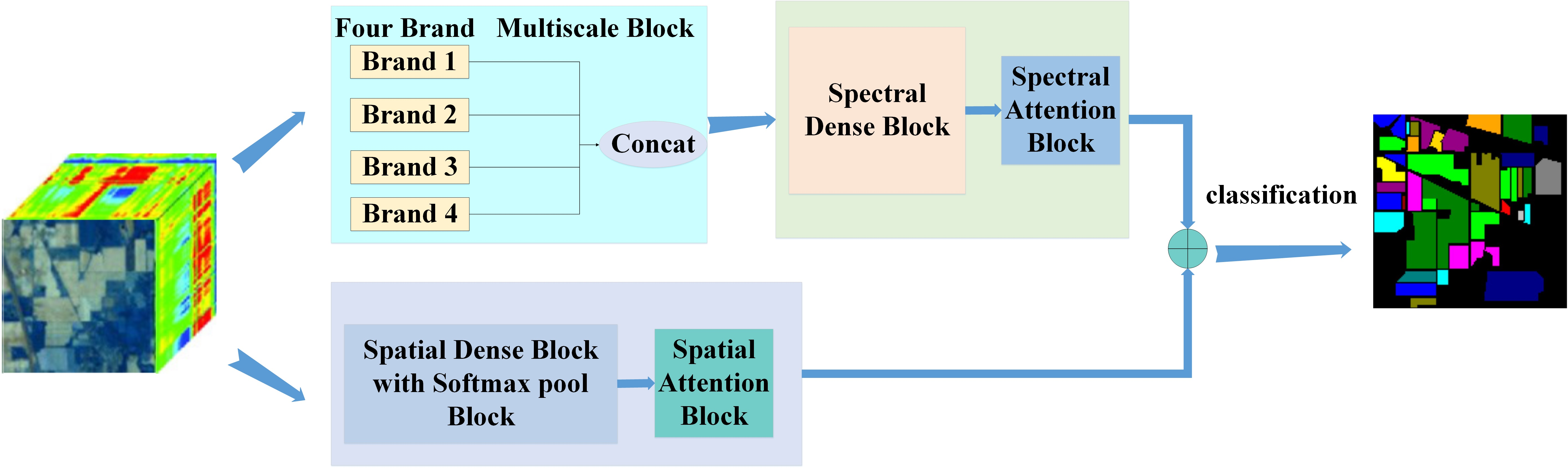
The overall framework of the proposed network based on spectral four branch multiscale network (SFBMSN) for hyperspectral image classification is shown in Figure 1.
The SFBMSN network is composed of three parts. In the first part, the FBMB structure with a channel attention module is designed to extract and select spectral features, so as to fully extract important spectral features. The second part uses the dense connection structure to further extract the spectral features and fully extract the information. In the third part, the dense connection structure of the first convolution layer including a 3D-Softpool module is used to extract spatial features, increase the receiving field of subsequent convolution and extract more spatial features, so as to improve the classification performance. In addition, some optimization strategies are used to prevent over fitting.
In the first part, FBMB includes four branches, and the convolution kernel size of each branch is not the same. A spectral attention mechanism is introduced into each branch to obtain spectral features more conducive to classification. Then, the spectral features extracted by four branches are fused. In the second part, based on the DenseNet [63] structure and the idea of reusing spectral features, the fused features are input into the DenseNet network, and the dense blocks with three convolution layers are used to extract spectral features. The third part is similar to the extraction of spectral features. The original hyperspectral data are input into the dense block containing 3D-Softpool. The 3D-Softpool module is added to the first convolution layer of dense blocks to extract spatial neighborhood features combined with spatial attention mechanism. Then, the feature maps obtained from spectral branches and spatial branches are added element by element, and the features after spatial–spectral fusion are input into global average pool (GAP), full connection layer and linear classifier to obtain the classification results.
2.2. FBMB and Spectral Self-Attention Module
The FBMB and spectral self-attention module are important modules in the first part of the proposed method. In Figure 1, the first part is the proposed FBMB structure with spectral self-attention mechanism. Firstly, principal component analysis (PCA) is performed on the original hyperspectral image data, and the data after PCA is , where 9 × 9 represents the length and width of the data, and band represents the number of channels of the data. Next, a three-dimensional convolution operation is carried out on the data . The size of the convolution kernel of the three-dimensional convolution layer is set to (1 × 1 × 7), the padding is set to (0 × 0 × 0) and the stride is set to (1 × 1 × 2). In this way, the length and width of the data after the convolution operation remain unchanged, which is 9 and 9, respectively, and the number of channels becomes , that is, is the number of channels of the data after the convolution layer operation.
The output data are input into the four branches of the FBMB module at the same time, and retain the useful spectral information as much as possible through the spectral self-attention mechanism in each branch. For the first branch of the FBMB module, the convolution layers with 6 convolution kernels are utilized for convolution. The population strategy is used for all branches to make the input and output data size consistent. After the convolution layer, the batch normalization (BN) layer is used. The BN layer can normalize and linearly scale the channel to speed up the convergence of the model. Suppose the input data are , the output data are and the trainable parameters are , then the process of BN can be represented as
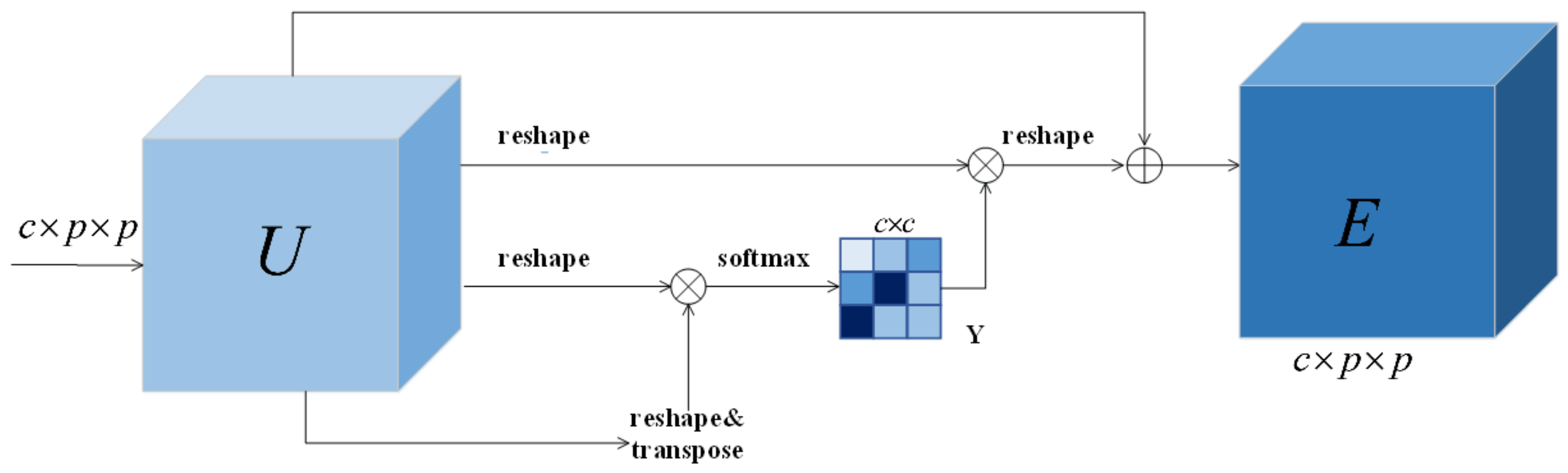
Firstly, the mean and variance of the input data are calculated according to Equations (1) and (2), then the input data are normalized to [0, 1] corresponding to Equation (3), and finally multiply each element in by and add to output . and are trainable parameters. The purpose of normalization is to adjust the data to a unified interval, reduce the divergence of data and reduce the learning difficulty of the network. Using BN and Mish activation function after convolution layer can effectively avoid gradient explosion and gradient disappearance. Then, continue to use the spectral self-attention mechanism to capture important spectral information. The schematic diagram of the mechanism of spectral self-attention is shown in Figure 2.
Using the spectral attention mechanism, we can mine the interdependence between spectral feature maps, extract feature maps with strong dependence, and improve the feature representation of specific semantics. As shown in Figure 2, represents the spectral features, which is the initial input of . Here, is the input patch size and represents the number of input channels. represents the spectral attention map, and the size of is . is calculated from the initial input spectral feature map . is used to measure the influence of the th spectral feature on the th spectral feature. is the th spectral feature and is the th spectral feature. The calculation process is
Then, the results of matrix multiplication between and are reshape into . Finally, the reshape result is weighted by the scale parameter, and input is added to obtain the final spectral attention map :
where is initialized to zero and can be learned gradually. The final map includes the weighted summations of features of all channels, which can improve the resolution of features.
In the second branch, the size of the convolution kernel in the first convolution layer is , the number of the convolution kernel is 6, and BN + Mish is used. The size of convolution kernel in the second convolution layer is , the number of convolution kernels is 6 and BN + Mish is used. At the end of the second branch, spectral self-attention is utilized, and the input size is . The third branch has the same structure as the fourth branch, and the size of convolution kernel is different. The size of convolution kernel in the third branch is and the number of convolution kernel is 6. For the fourth branch, the size of convolution kernel is and the number of convolution kernel is 6. After the convolution layer, BN + Mish and spectral self-attention mechanism are adopted to avoid data explosion and gradient disappearance. Because data padding is used in all four branches, the output size is . Finally, the data outputs from the four branches are added, and the added cube size is . The cube output by the FBMB module contains a large amount of important spectral feature information, which provides rich spectral feature information for subsequent operations.
2.3. Dense Connection Network
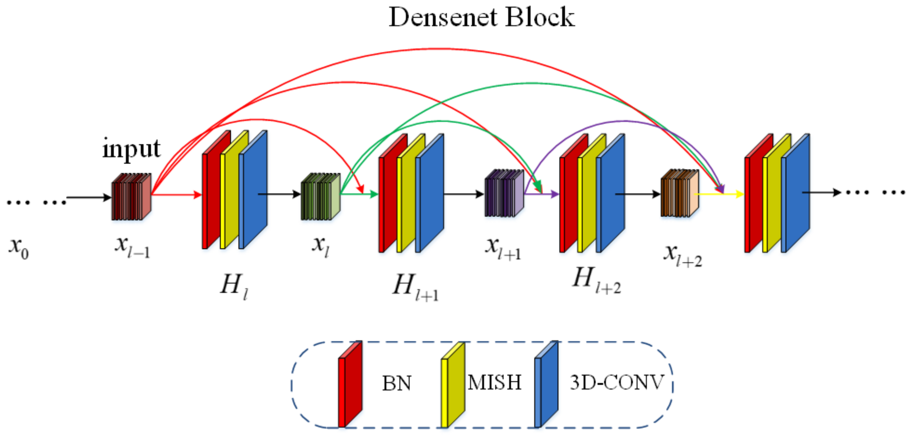
Dense connection network is an important network of the second and third parts of the proposed method. In order to avoid the gradient disappearance problem caused by the deepening of the network depth, the dense connection module is adopted behind the FBMB module to further extract the effective spectral features. On the premise of ensuring full transmission of information between the middle layers of the network, all layers are directly connected. Each layer connects the inputs of all previous layers, and then transmits those output feature maps to all subsequent layers. This can ensure the maximum spectral information flow between network layers and make full use of spectral features. The structure diagram of DenseNet is shown in Figure 3.
DenseNet used in this paper has three layers, and each layer is composed of convolution, BN, and Mish. Each layer has a nonlinear transformation function . is the combined function of the three operations. is the output of layer . In the traditional feedback network, the output of layer is the input of layer , and the output of layer can be obtained, which can be represented as
DenseNet can effectively improve inter layer information transmission by connecting one layer with all subsequent layers. Therefore, the output of all layers before layer is used as the input of layer , and the output of layer is represented as
After dense connection, the key information of spectral features is extracted by spectral self-attention mechanism again.
2.4. Spatial Dense Connection Network with 3D-Softpool
As dense connection network has already been introduced, it will not be repeated in this section. 3D-Softpool is an important module in the third part of the proposed method. The principle of 3D-Softpool will be introduced in detail in this section. The dense connection is utilized to capture spatial features. This dense connection has three layers, and each layer is composed of convolution, BN and Mish. The Mish layer is replaced with 3D-Softpool in the first layer of dense connection. 3D-Softpool is a fast and efficient pooling method, which accumulates activation in an exponentially weighted manner. Compared to other pooling methods, 3D-Softpool retains more information during the down sampling activation mapping, which helps to improve classification performance. 3D-Softpool is based on the natural index (e), which can result in a large activation value and have a greater impact on the output. 3D-Softpool is differentiable, which means that all activation in the local neighborhood will be assigned at least one minimum gradient value during back propagation. The process of 3D-Softpool is shown in Figure 4.
3D-Softpool uses the maximum approximation in the activation area, and each activation is assigned a weight , which can be represented as
The output value of 3D-Softpool is obtained by summing all weighted activation in an activation map:
The output is
The probability distribution of the normalized results generated using SoftMax is proportional to the adjacent activation value of each activation value relative to the adjacent region. It can make all activation contribute to the final classification output, extract more useful spatial features and improve the classification accuracy.
2.5. Spatial Self-Attention Mechanism
The spatial self-attention mechanism is an important module in the third part of the proposed method. The principle of spatial self-attention mechanism will be introduced in detail in this section. The data generated after 3D-Conv, BN and Mish operations are input to the spatial self-attention module. For spatial attention mechanism, by establishing the context relationships between local spatial features, more extensive context information can be encoded into local spatial features to improve the representation ability of features. The spatial self-attention mechanism is shown in Figure 5.
is the input feature map, , and are three new spatial feature maps generated after three convolution operations, among which . Then , and are reshaped into , where and represent the number of pixels. and perform matrix multiplication, and then obtain the spatial attention feature map through SoftMax layer calculation.
where, is the influence of the th pixel on the th pixel. and perform matrix multiplication, and the result is reshaped into ;
Among them, the initial value of is zero, which can gradually assign more weights. By observing Equation (13), we can find that all positions and original input feature maps will be added with a certain weight to obtain the final output spatial attention feature map .
3. Experiment and Results
3.1. Data Set and Parameter Setting
The performance of the proposed method is verified by using four classical hyperspectral image data sets: Indian pine (IN), Pavia University (UP), Kennedy Space Center (KSC) and Salinas Valley (SV).
The IN data set shown in Table 1 is the earliest test data used for hyperspectral image classification. An Indian pine tree in Indiana was imaged by airborne visible infrared imaging spectrometer (AVIRIS) in 1992, and then intercepted with a size of 145 × 145. The size of 145 is labeled for hyperspectral image classification test. The spatial resolution of the image generated by the spectral imager is about 20 m. After eliminating useless bands, 200 bands are left for experimental research. There are 21,025 pixels in the data set, but only 10,249 pixels are ground object pixels, and the remaining 10,776 pixels are background pixels. In the actual classification, these pixels need to be eliminated. Because the intercepted area is crops, there are 16 classes in total, so different ground objects have relatively similar spectral curves, and in these 16 classes, the distribution of samples is extremely uneven.
The UP data set shown in Table 2 is part of the hyperspectral data imaged by the airborne reflective optical system imaging spectrometer (rosis) of Germany in Pavia City, Italy in 2003. The spatial resolution of the image is 1.3 m and the data size is 610 × 340; The spectral imager imaged 115 bands in the wavelength range of 0.43–0.86 μm, eliminated 12 bands affected by noise, and left 103 available bands. Among them, the data set contains 9 types of features, including trees, asphalt roads, bricks, meadows, etc.
The KSC data set shown in Table 3 represent the data collected by NASA AVIRIS (airborne visible/infrared imaging spectrometer) instrument at Kennedy Space Center (KSC) in Florida on 23 March 1996. AVIRIS collected 224 bands with a width of 10 nm and a central wavelength of 400–2500 nm. The spatial resolution of KSC data obtained from an altitude of about 20 km is 18 M. After removing the water absorption and low SNR bands, 176 bands were used for analysis. Training data were selected using land cover maps provided by color infrared photography and Landsat thermal mapper (TM) images provided by Kennedy Space Center. The vegetation classification scheme was developed by KSC personnel to define the types of functions that can be distinguished at the spatial resolution of Landsat and these AVIRIS data. Because the spectral characteristics of some vegetation types are similar, it is difficult to distinguish land cover in this environment. For classification purposes, 13 categories are defined for the site, representing various land cover types that occur in this environment.
The SV data set shown in Table 4 is the same as the Indian pines image. The Salinas data were also obtained by AVIRIS imaging spectrometer, which is an image of the Salinas Valley in California, USA. Different from Indian pines, its spatial resolution reaches 3.7 m. The image originally has 224 bands. Similarly, we generally use the image of the remaining 204 bands after excluding the 108-112154-167 and the 224th band that cannot be reflected by water. The size of the image is 512 × 217. Therefore, it contains 111,104 pixels, of which 56,975 pixels are background pixels, and 54,129 pixels can be applied to classification. These pixels are divided into 16 categories, including fallow and celery.
In the experiment, in order to verify that small training samples can also achieve high classification accuracy, we randomly selected 3%, 0.5%, 3% and 0.5% samples in IN, UP, KSC and SV for training, and the remaining samples in each data set were used for testing. The next section will prove that the proposed method can achieve high classification accuracy in the case of small samples. Table 1, Table 2, Table 3 and Table 4 show the number of training samples and test samples in the four data sets of IN, UP, KSC and SV.
The experimental hardware platform is a server with NVIDIA GeForceRTX2060 GPU and 16 GB random access memory. The experimental software platform is based on Windows 10 VisualStudioCode operating system, using CUDA 10.0, Pytorch 1.2.0 and Python 3.7.4. All experiments randomly selected different training data and were repeated 10 times. The final results of all experiments were the average results of 10 experiments. The experiment uses Adam optimizer, and the learning rate is set to 0.0001. We used real positive (TP) to represent the positive samples correctly classified by the model, false negative (FN) to represent the positive samples incorrectly classified by the model, false positive (FP) to represent the negative samples incorrectly classified by the model, and true negative (TN) to represent the negative samples correctly classified by the model. The overall accuracy (OA), average accuracy (AA) and Kappa coefficient (Kappa) were used as evaluation indexes [64]. OA is the ratio of the number of correctly classified samples to the total number of samples. The OA is calculated as
AA is the classification accuracy of each category. The calculation of AA is
Kappa coefficient measures the consistency between classification map and ground real map. The calculation of Kappa is
where is the sum of the number of correctly classified samples of each category divided by the total number of samples; is the actual quantity of each category multiplied by the sum of the predicted quantity of this category divided by the square of the total number of all categories.
Some traditional and advanced hyperspectral image classification methods based on convolutional neural network are used to compare the classification performance with the proposed method. These methods include SVM, CDCNN, SSRN, FDSSC, DBMA, and DBDA. SVM uses radial basis function to solve nonlinear classification problem; CDCNN is a 2D-CNN model. Other methods and proposed methods are 3D-CNN model.
The design of network structure and the selection of parameters determine the classification performance of the network. In our experiments, the main parameters of SFBMSN are shown in Table 5. Hyperspectral images data are dimensionally reduced by PCA, and then put into the network for feature extraction. Assuming that the size of the input data is , the data pass through the input module, FBMB module of spectral branch, 3D-Softpool module of spatial branch, dense connection block, attention block and final classification block. Obviously, spatial size and are important factors affecting the classification performance. Therefore, this section will analyze the impact of these parameters in detail. Table 5 shows the parameter configurations of the proposed methods.
Effect of on classification performance: determines the depth of the network. Here, the influence of parameter in spectral branch on the classification accuracy is discussed. Generally speaking, with the increase in network depth, the classification accuracy will also improve. Too many layers will bring problems such as over fitting, gradient disappearance and gradient explosion. Figure 6 shows the impact of the number of on OA of different data sets. Set of IN, UP, KSC, and SV data sets to 96, 97, 98 and 99, respectively, and the spatial size is fixed. As can be seen from Figure 6a, when is set to 97, the OA value is the highest, and OA gradually decreases with the increase in . For SV data set, OA value will fluctuate slightly with the increase in . In order to avoid information redundancy caused by excessively densely connected networks and balance classification accuracy and calculation, the number of IN, UP, SV and KSC data sets is set to 97.
Effect of spatial size on classification performance: For hyperspectral images, too small input data blocks will lead to insufficient feature extraction, while large data blocks easily result in noise problems. Therefore, the spatial size of the input 3D data block will also affect the classification accuracy. When is fixed, the effect of spatial size on classification performance is analyzed. The spatial size of the input sample is set to , , , , and , respectively. Figure 6b shows the OAs with different input spatial sizes on four data sets. As can be seen from Figure 6b, the OA increases with the increase in spatial size. For UP and IN data sets, when the spatial size reaches , the OA accuracy begins to decrease. For SV and KSC data sets, when the spatial size reaches , the OA is the highest. Therefore, the input block with spatial size is selected to train the network.
3.2. Experimental Results and Analysis
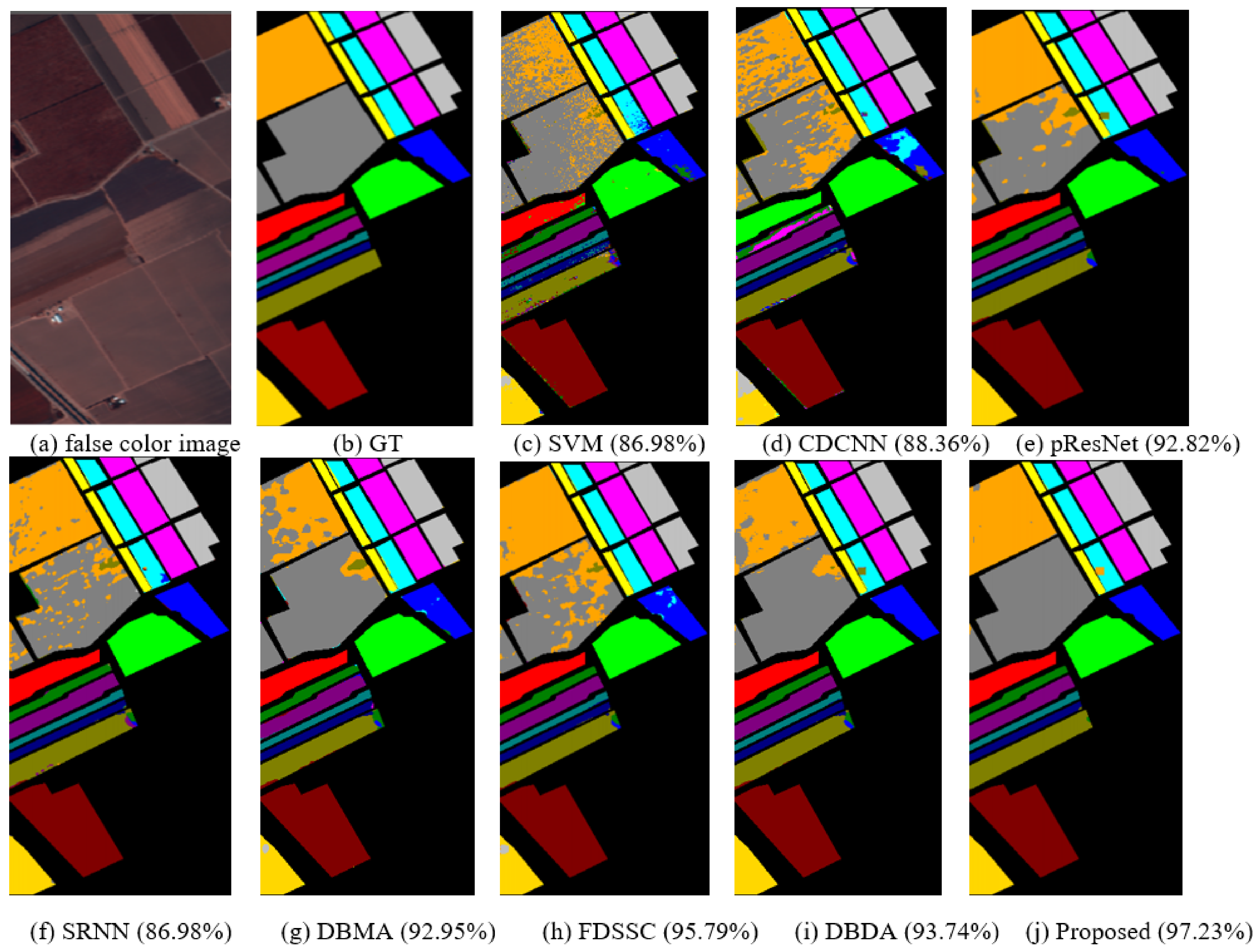
All methods are tested with the same proportion of training samples, and the classification performance of these methods is compared. Table 6, Table 7, Table 8 and Table 9 lists the classification accuracy of all categories obtained by all methods on the four data sets of IN, UP, KSC and SV. All results obtain the average of the experimental results 10 times, and the highest classification results are shown in bold. It can be observed from Table 6, Table 7, Table 8 and Table 9 that compared with other methods, OA, AA and Kappa proposed by the method are all the highest. The OA value of the proposed method is 28.29% higher than that of SVM, and 6.11%, 3.45%, 6.82%, 24.64%, 3.77% and 9.9% higher than that of DBMA, DBDA, SSRN, CDCNN, FDSSC and pResNet, respectively. SVM does not use spatial neighborhood information and has poor robustness, so its OA value is low at only 67.77%. CDCNN is a 2D-CNN structure, and its robustness is better than SVM, so its OA value is 3.65% higher than that of SVM. FDSSC adopts the dense connection, and its OA value is more than 3.05% higher than that of SSRN using the residual connection. The DBMA method adopts the network structure of double branches and double attention, and using small sample training will lead to over fitting. The DBDA network uses double branch and double attention structure, which has a more flexible feature extraction structure than the DBMA network. Therefore, the OA value obtained by DBDA is higher than that of DBMA. The proposed method designs the FBMB module to extract spectral features. The convolution kernels of different sizes are used to fully extract the important spectral features on the four branches, and the spectral attention mechanism is deployed on each branch to further extract the key spectral features. Finally, the spectral features extracted from the four branches are fused to obtain more effective spectral features. Observation of the experimental results shows that the classification performance is significantly improved after using the 3D-Softpool module to extract spatial features. After observing the experimental results of classification using small samples, it is found that the proposed method has the best classification performance. As can be seen from Table 6, Table 7, Table 8 and Table 9, the classification accuracy of the proposed method is the highest among the four data sets. The experimental results also show that the classification performance of the CDCNN method using the shallow network to capture features is the worst, the receptive field of the shallow network is smaller than that of the deep network and it extracts low-level features. Other methods used for comparison also adopt feature fusion strategies, including SSAN and FDSSC, which usually provide higher classification accuracy than other methods (CDCNN, SVM). When using small samples for training, the hierarchical fusion mechanism can fuse the complementary information and related information output from different convolution layers, making the extracted features more comprehensive. Moreover, in order to further verify the performance of the proposed SFBMSN network, the classification maps of different methods on the four data sets of IN, UP, SV and KSC are shown in Figure 7, Figure 8, Figure 9 and Figure 10. By observing the classification map, it can be seen that compared with the classification map of other methods, the classification map of the proposed method has less noise, clear boundary and is closest to the ground truth map. The effectiveness of the proposed method is further proved.
4. Discussion
Experiment 1: In order to verify the effectiveness of the proposed attention block, FBMB module, 3D-Softpool and dense connection, some ablation experiments were carried out on four hyperspectral images data sets. Only the modules to be tested in the network were deleted, and other parts remained unchanged. Figure 11 shows the experimental results with or without specific modules. At the same time, it can be seen that the accuracy of the network reaches the highest after adding the spatial and spectral attention module. The reason is that the introduction of attention block to extract the features of hyperspectral images can adaptively allocate different weights, different spectral features and different spatial regions and selectively enhance the important features useful for classification, that is, increase the weight of some important features, which will help to improve the accuracy of classification. In addition, Figure 11b shows the effectiveness of fusing spatial–spectral features of different scales. As shown in Figure 11b, the FBMB module improves the classification accuracy of four data sets. This is because multiple branches can effectively extract spectral features of different scales, which is helpful to improve the classification accuracy. It is obvious from Figure 11c that after removing the 3D-Softpool module, the OAs on the four data sets decrease significantly. 3D-Softpool block can reduce the loss of information in feature mapping and retain more information in down sampling activation mapping, so better classification results can be achieved on four data sets. As can be seen from Figure 11d, if the dense connection is not used for the experiment, the OAS on the four data sets of IN, UP, SV and KSC decreases significantly. Using dense connection, all convolution layers can be connected, so that the spectral characteristic map output after convolution operation of each convolution layer is the input of all subsequent layers. This can ensure the maximum spectral information flow between network layers and make full use of spectral features. Therefore, better classification performance can be obtained on the four data sets of IN, UP, SV and KSC. As can be seen from Figure 11d, if the dense connection is not adopted for the experiment, the OAs on the four data sets of IN, UP, SV and KSC decreases significantly. Using dense connection, all convolution layers can be connected, so that the spectral feature maps output by each convolution layer are the input of all subsequent layers. This can ensure the maximum spectral information flow between network layers and make full use of spectral features. Therefore, better classification performance can be obtained on the four data sets of IN, UP, SV and KSC.
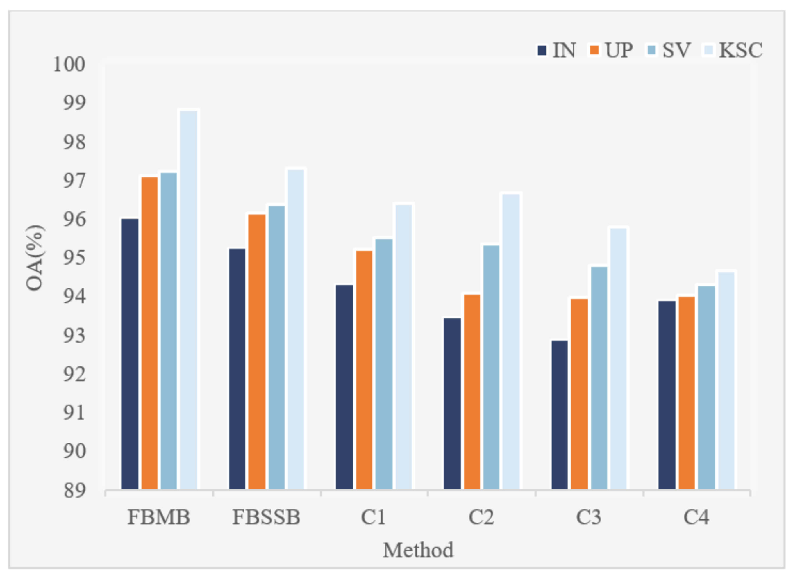
Experiment 2: Figure 12 is the schematic diagram of FBMB. In order to prove that our proposed FBMB can effectively improve the classification performance of hyperspectral image classification we carried out two groups of comparative experiments. Only the structure of FBMB was changed, and other structures remained unchanged. Some comparative experiments were carried out under the same conditions. The experimental results of the two groups of experiments were compared with that of the proposed method. In the first experiment, the convolution kernel size of all convolutions in FBMB were set to 7 × 7 × 7. We call the first group of comparative experiments the four-branch same scale block (FBSSB). In the second experiment, we used any three branches of the four branches B1, B2, B3 and B4 for experiments, which can have four combinations, namely C1 (B1, B2, B3), C2 (B1, B2, B4), C3 (B2, B3, B4) and C4 (B1, B3, B4). The experimental results of the three groups of comparative experiments on the four data sets of IN, UP, SV and KSC are shown in Figure 13. As can be seen from Figure 13, FBMB has the highest OA value and the best classification performance on the four data sets. The convolution kernel size of all convolutions in the first group of experiments is 7 × 7 × 7. The classification performance of this structure is not good. The size of convolution kernel is large, which leads to large number of parameters and slow operation in the experimental process. Compared with the combination of three branches, the feature extraction of four branches in FBMB is more sufficient and the classification performance is better.
Experiment 3: In order to further verify the performance of the proposed method, in comparison with other methods, the classification performance of different methods under different proportions of training samples was compared. In the experiment, the training ratios of IN, UP, KSC and SV were set to 1%, 5%, 10% and 15%, respectively. The experimental results are shown in Figure 14. As can be seen from Figure 14, when there are few training samples, the classification performance of CDCNN and SVM is relatively poor, and the classification performance of the proposed method is the best. With the increase in the number of samples, each method can obtain higher classification accuracy, but the classification accuracy of the proposed method can still be higher than that of other methods. This shows that this method has good generalization ability.
Experiment 4: Feature fusion merges the features extracted from the image into a complete image as the input of the next layer network, which can input more discriminative features for the next layer network. According to the order of fusion and prediction, feature fusion can be divided into early feature fusion and late feature fusion. Early feature fusion is a commonly used classical feature fusion method. For example, in an Inside–Outside Net (ION) [65] or HyperNet [66]), concatenation [67] or addition operations are used to fuse certain layers. The feature fusion strategy in this experiment is an early fusion strategy that directly connects two spectral and spatial scale features. The two input features have the same size, and the output feature dimension is the sum of the two dimensions. Table 10 shows the experimental results of whether to use the fusion strategy. It can be seen from Table 10 that the OA values obtained on the four data sets after feature fusion are significantly higher than those obtained without feature fusion strategy. After feature fusion is used on each data set, the OA value obtained increases by more than 1.8%. The results show that the processing effect of feature fusion strategy on hyperspectral image classification is significantly improved compared with that without feature fusion strategy.
5. Conclusions
In this paper, the SFBMSN method is proposed for hyperspectral image classification. The FBMB module, 3D-Softpool module, spatial attention module, channel attention module and dense connection are used in the network structure of this method. Using FBMB module, the spectral features of hyperspectral images can be extracted from multiple scales and different levels, and the spectral attention module is introduced into each branch of FBMB to obtain more important information and suppress useless information. Using a dense connection structure to extract spatial features can directly splice spatial features from different layers, realize feature reuse and improve the efficiency of feature extraction. The 3D-Softpool module is used for the first time in the dense connection structure. The 3D-Softpool can retain more spatial feature information in the down sampling activation mapping. The purpose of using spatial attention is to extract important spatial information and suppress useless redundant information. Experiments on four commonly used data sets using small training samples show that the proposed SFBMSN method is very competitive in hyperspectral image classification tasks.
In future research, we will further explore how to fuse the extracted spatial–spectral features more effectively, so that the spatial and spectral features at the edge can also be fully applied to classification. Therefore, designing a more efficient fusion model is an important direction of our future research.
Author Contributions
Conceptualization, C.S.; data curation, C.S. and J.S.; formal analysis, J.S.; methodology, C.S.; software, J.S.; validation, C.S. and J.S.; writing—original draft, J.S.; writing—review and editing, C.S. and L.W. All authors have read and agreed to the published version of the manuscript.
Funding
This research was funded in part by the National Natural Science Foundation of China (41701479, 62071084), in part by the Heilongjiang Science Foundation Project of China under Grant LH2021D022, and in part by the Fundamental Research Funds in Heilongjiang Provincial Universities of China under Grant 135509136.
Institutional Review Board Statement
Not applicable.
Informed Consent Statement
Not applicable.
Data Availability Statement
The Indiana Pines, University of Pavia, Kennedy Space Center and Salinas Valley data sets are available online at http://www.ehu.eus/ccwintco/index.php?title=Hyperspectral_Remote_Sensing_Scenes (accessed on 3 July 2021).
Acknowledgments
The authors would like to thank the editors and the reviewers for their help and suggestions.
Conflicts of Interest
The authors declare no conflict of interest.
References
- Chang, C.I. Hyperspectral Data Exploitation: Theory and Applications; John Wiley & Sons: Hoboken, NJ, USA, 2007. [Google Scholar] [CrossRef] [Green Version]
- Patel, N.K.; Patnaik, C.; Dutta, S.; Shekh, A.M.; Dave, A.J. Study of crop growth parameters using airborne imaging spectrometer data. Int. J. Remote Sens. 2001, 22, 2401–2411. [Google Scholar] [CrossRef]
- Goetz, A.F.; Vane, G.; Solomon, J.E.; Rock, B.N. Imaging Spectrometry for Earth Remote Sensing. Science 1985, 228, 1147–1153. [Google Scholar] [CrossRef] [PubMed]
- Civco, D.L. Artifificial neural networks for land-cover classification and mapping. Int. J. Geogr. Inf. Syst. 1993, 7, 173–186. [Google Scholar] [CrossRef]
- Wang, X.; Kong, Y.; Gao, Y.; Cheng, Y. Dimensionality reduction for hyperspectral data based on pairwise constraint discriminative analysis and nonnegative sparse divergence. IEEE J. Sel. Top. Appl. Earth Obs. Remote Sens. 2017, 10, 1552–1562. [Google Scholar] [CrossRef]
- Ghamisi, P.; Benediktsson, J.A.; Ulfarsson, M.O. Spectral–Spatial Classification of Hyperspectral Images Based on Hidden Markov Random Fields. IEEE Trans. Geosci. Remote Sens. 2013, 52, 2565–2574. [Google Scholar] [CrossRef] [Green Version]
- Farrugia, R.A.; Debono, C.J. A Robust Error Detection Mechanism for H.264/AVC Coded Video Sequences Based on Support Vector Machines. IEEE Trans. Circuits Syst. Video Technol. 2008, 18, 1766–1770. [Google Scholar] [CrossRef] [Green Version]
- Zhong, P.; Wang, R. Jointly Learning the Hybrid CRF and MLR Model for Simultaneous Denoising and Classification of Hyperspectral Imagery. IEEE Trans. Neural Netw. Learn. Syst. 2014, 25, 1319–1334. [Google Scholar] [CrossRef]
- Fang, L.; Li, S.; Kang, X.; Benediktsson, J.A. Spectral-spatial classification of hyperspectral images with a superpixel-based discriminative sparse model. IEEE Trans. Geosci. Remote Sens. 2015, 53, 4186–4201. [Google Scholar] [CrossRef]
- Fu, W.; Li, S.; Fang, L. Spectral-spatial hyperspectral image classification via superpixel merging and sparse representation. In Proceedings of the 2015 IEEE International Geoscience and Remote Sensing Symposium (IGARSS), Milan, Italy, 26–31 July 2015; pp. 4971–4974. [Google Scholar] [CrossRef]
- Fang, L.; Li, S.; Duan, W.; Ren, J.; Benediktsson, J.A. Classification of Hyperspectral Images by Exploiting Spectral–Spatial Information of Superpixel via Multiple Kernels. IEEE Trans. Geosci. Remote Sens. 2015, 53, 6663–6674. [Google Scholar] [CrossRef] [Green Version]
- Li, G.; Li, L.; Zhu, H.; Liu, X.; Jiao, L. Adaptive Multiscale Deep Fusion Residual Network for Remote Sensing Image Classification. IEEE Trans. Geosci. Remote Sens. 2019, 57, 8506–8521. [Google Scholar] [CrossRef]
- Ronneberger, O.; Fischer, P.; Brox, T. U-Net: Convolutional Networks for Biomedical Image Segmentation. In International Conference on Medical Image Computing and Computer-Assisted Intervention; Springer: Cham, Switzerland, 2015; pp. 234–241. [Google Scholar] [CrossRef] [Green Version]
- Wang, R.J.; Li, X.; Ling, C.X. Pelee: A Real-Time Object Detection System on Mobile Devices. arXiv 2018, arXiv:1804.06882. [Google Scholar]
- Zeng, D.; Liu, K.; Chen, Y.; Zhao, J. Distant Supervision for Relation Extraction via Piecewise Convolutional Neural Networks. In Proceedings of the 2015 Conference on Empirical Methods in Natural Language Processing, Lisbon, Portugal, 17–21 September 2015; pp. 1753–1762. [Google Scholar] [CrossRef]
- Gehring, J.; Auli, M.; Grangier, D.; Yarats, D.; Dauphin, Y.N. Convolutional Sequence to Sequence Learning. arXiv 2017, arXiv:1705.03122. [Google Scholar]
- He, H.; Gimpel, K.; Lin, J. Multi-Perspective Sentence Similarity Modeling with Convolutional Neural Networks. In Proceedings of the 2015 Conference on Empirical Methods in Natural Language Processing, Milan, Italy, 26–31 July 2015; pp. 1576–1586. [Google Scholar] [CrossRef]
- He, L.; Li, J.; Liu, C.; Li, S. Recent advances on spectral–spatial hyperspectral image classification: An overview and new guidelines. IEEE Trans. Geosci. Remote Sens. 2018, 56, 1579–1597. [Google Scholar] [CrossRef]
- Shen, L.; Jia, S. Three-dimensional Gabor wavelets for pixel-based hyperspectral imagery classification. IEEE Trans. Geosci. Remote Sens. 2011, 49, 5039–5046. [Google Scholar] [CrossRef]
- Tang, Y.; Lu, Y.; Yuan, H. Hyperspectral image classification based on three-dimensional scattering wavelet transform. IEEE Trans. Geosci. Remote Sens. 2015, 53, 2467–2480. [Google Scholar] [CrossRef]
- Phillips, R.D.; Blinn, C.E.; Watson, L.T.; Wynne, R.H. An adaptive noise-fifiltering algorithm for AVIRIS data with implications for classi- fification accuracy. IEEE Trans. Geosci.Remote Sens. 2009, 47, 3168–3179. [Google Scholar] [CrossRef]
- Palmason, J.A.; Benediktsson, J.A.; Sveinsson, J.R.; Chanussot, J. Classification of hyperspectral data from urban areas using morphological preprocessing and independent component analysis. In Proceedings of the 2005 IEEE International Geoscience and Remote Sensing Symposium, 2005. IGARSS ’05, Seoul, Korea, 29 July 2005; p. 4. [Google Scholar] [CrossRef]
- Li, J.; Marpu, P.R.; Plaza, A.; Bioucas-Dias, J.M.; Benediktsson, J.A. Generalized composite kernel framework for hyperspectral image classification. IEEE Trans. Geosci. Remote Sens. 2013, 51, 4816–4829. [Google Scholar] [CrossRef]
- Hong, D.; Wu, X.; Ghamisi, P.; Chanussot, J.; Yokoya, N.; Zhu, X.X. Invariant attribute profifiles: A spatial-frequency joint feature extractor for hyperspectral image classification. IEEE Trans. Geosci. Remote Sens. 2020, 58, 3791–3808. [Google Scholar] [CrossRef] [Green Version]
- Duan, P.; Kang, X.; Li, S.; Ghamisi, P.; Benediktsson, J.A. Fusion of multiple edge-preserving operations for hyperspectral image classification. IEEE Trans. Geosci. Remote Sens. 2019, 57, 10336–10349. [Google Scholar] [CrossRef]
- Sun, L.; Wu, Z.; Liu, J.; Xiao, L.; Wei, Z. Supervised spectral–spatial hyperspectral image classification with weighted Markov random fifields. IEEE Trans. Geosci. Remote Sens. 2015, 53, 1490–1503. [Google Scholar] [CrossRef]
- Li, F.; Xu, L.; Siva, P.; Wong, A.; Clausi, D.A. Hyperspectral image classification with limited labeled training samples using enhanced ensemble learning and conditional random fifields. IEEE J. Sel. Top. Appl. Earth Obs. Remote Sens. 2015, 8, 2427–2438. [Google Scholar] [CrossRef]
- Chen, Y.; Nasrabadi, N.M.; Tran, T.D. Hyperspectral image classification using dictionary-based sparse representation. IEEE Trans. Geosci. Remote Sens. 2011, 49, 3973–3985. [Google Scholar] [CrossRef]
- Gao, L.; Hong, D.; Yao, J.; Zhang, B.; Gamba, P.; Chanussot, J. Spectral superresolution of multispectral imagery with joint sparse and lowrank learning. IEEE Trans. Geosci. Remote Sens. 2020, 59, 2269–2280. [Google Scholar] [CrossRef]
- Ghamisi, P.; Couceiro, M.S.; Martins, F.M.L.; Benediktsson, J.A. Multilevel image segmentation based on fractional-order Darwinian particle swarm optimization. IEEE Trans. Geosci. Remote Sens. 2014, 52, 2382–2394. [Google Scholar] [CrossRef] [Green Version]
- Hong, D.; Gao, L.; Yokoya, N.; Yao, J.; Chanussot, J.; Du, Q.; Zhang, B. More diverse means better: Multimodal deep learning meets remote-sensing imagery classification. IEEE Trans. Geosci. Remote Sens. 2020, 59, 4340–4354. [Google Scholar] [CrossRef]
- Zheng, K.; Gao, L.; Liao, W.; Hong, D.; Zhang, B.; Cui, X.; Chanussot, J. Coupled convolutional neural network with adaptive response function learning for unsupervised hyperspectral superresolution. IEEE Trans. Geosci. Remote Sens. 2020, 59, 2487–2502. [Google Scholar] [CrossRef]
- Chen, Y.; Lin, Z.; Zhao, X.; Wang, G.; Gu, Y. Deep learning-based classification of hyperspectral data. IEEE J. Sel. Top. Appl. Earth Obs. Remote Sens. 2014, 7, 2094–2107. [Google Scholar] [CrossRef]
- Chen, Y.; Zhao, X.; Jia, X. Spectral–Spatial classification of hyperspectral data based on deep belief network. IEEE J. Sel. Top. Appl. Earth Obs. Remote Sens. 2015, 8, 2381–2392. [Google Scholar] [CrossRef]
- Mou, L.; Ghamisi, P.; Zhu, X.X. Deep recurrent neural networks for hyperspectral image classification. IEEE Trans. Geosci. Remote Sens. 2017, 55, 3639–3655. [Google Scholar] [CrossRef] [Green Version]
- Hang, R.; Liu, Q.; Hong, D.; Ghamisi, P. Cascaded recurrent neural networks for hyperspectral image classification. IEEE Trans. Geosci. Remote Sens. 2019, 57, 5384–5394. [Google Scholar] [CrossRef] [Green Version]
- Hong, D.; Gao, L.; Yao, J.; Zhang, B.; Plaza, A.; Chanussot, J. Graph convolutional networks for hyperspectral image classification. IEEE Trans. Geosci. Remote Sens. 2020, 59, 5966–5978. [Google Scholar] [CrossRef]
- Tao, C.; Pan, H.; Li, Y.; Zou, Z. Unsupervised spectral-spatial feature learning with stacked sparse autoencoder for hyperspectral imagery classification. IEEE Geosci. Remote Sens. Lett. 2015, 12, 2438–2442. [Google Scholar] [CrossRef]
- Ma, X.; Wang, H.; Geng, J. Spectral-spatial classification of hyperspectral image based on deep auto-encoder. IEEE J. Sel. Top. Appl. Earth Obs. Remote Sens. 2016, 9, 4073–4085. [Google Scholar] [CrossRef]
- Zhang, X.; Liang, Y.; Li, C.; Hu, N.; Jiao, L.; Zhou, H. Recursive autoencoders-based unsupervised feature learning for hyperspectral image classification. IEEE Geosci. Remote Sens. Lett. 2017, 14, 1928–1932. [Google Scholar] [CrossRef] [Green Version]
- Hu, W.; Huang, Y.; Wei, L.; Zhang, F.; Li, H.-C. Deep Convolutional Neural Networks for Hyperspectral Image Classification. J. Sens. 2015, 2015, 258619. [Google Scholar] [CrossRef] [Green Version]
- Li, W.; Wu, G.; Zhang, F.; Du, Q. Hyperspectral Image Classification Using Deep Pixel-Pair Features. IEEE Trans. Geosci. Remote Sens. 2016, 55, 844–853. [Google Scholar] [CrossRef]
- Fang, L.; Liu, Z.; Song, W. Deep Hashing Neural Networks for Hyperspectral Image Feature Extraction. IEEE Geosci. Remote Sens. Lett. 2019, 16, 1412–1416. [Google Scholar] [CrossRef]
- Chen, Y.; Li, C.; Ghamisi, P.; Jia, X.; Gu, Y. Deep Fusion of Remote Sensing Data for Accurate Classification. IEEE Geosci. Remote Sens. Lett. 2017, 14, 1253–1257. [Google Scholar] [CrossRef]
- Zhang, M.; Li, W.; Du, Q. Diverse Region-Based CNN for Hyperspectral Image Classification. IEEE Trans. Image Process. 2018, 27, 2623–2634. [Google Scholar] [CrossRef]
- Zhu, J.; Fang, L.; Ghamisi, P. Deformable Convolutional Neural Networks for Hyperspectral Image Classification. IEEE Geosci. Remote Sens. Lett. 2018, 15, 1254–1258. [Google Scholar] [CrossRef]
- Ding, X.; Zhang, X.; Han, J.; Ding, G. Diverse Branch Block: Building a Convolution as an Inception-like Unit.Computer Science.Computer Vision and Pattern Recognition. arXiv 2021, arXiv:2103.13425v2. [Google Scholar]
- Stergiou, A.; Poppe, R.; Kalliatakis, G. Refining activation downsampling with SoftPool. Computer Science.Computer Vision and Pattern Recognition. arXiv 2021, arXiv:2101.00440v3. [Google Scholar]
- Li, R.; Zheng, S.; Duan, C.; Yang, Y.; Wang, X. Classification of hyperspectral image based on double-branch dual-attention mechanism network. Remote Sens. 2020, 12, 582. [Google Scholar] [CrossRef] [Green Version]
- Chen, Y.; Jiang, H.; Li, C.; Jia, X.; Ghamisi, P. Deep Feature Extraction and Classification of Hyperspectral Images Based on Convolutional Neural Networks. IEEE Trans. Geosci. Remote Sens. 2016, 54, 6232–6251. [Google Scholar] [CrossRef] [Green Version]
- Liu, B.; Yu, X.; Zhang, P.; Tan, X.; Wang, R.; Zhi, L. Spectral-spatial classification of hyperspectral image using three-dimensional convolution network. J. Appl. Remote Sens. 2018, 12, 016005. [Google Scholar] [CrossRef]
- Li, Y.; Zhang, H.; Shen, Q. Spectral-Spatial Classification of Hyperspectral Imagery with 3D Convolutional Neural Network. Remote Sens. 2017, 9, 67. [Google Scholar] [CrossRef] [Green Version]
- Paoletti, M.E.; Haut, J.M.; Fernandez-Beltran, R.; Plaza, J.; Plaza, A.J.; Pla, F. Deep pyramidal residual networks for spectral–spatial hyperspectral image classification. IEEE Trans. Geosci. Remote Sens. 2019, 57, 740–754. [Google Scholar] [CrossRef]
- Wang, W.; Dou, S.; Jiang, Z.; Sun, L. A fast dense spectral–spatial convolution network framework for hyperspectral images classification. Remote Sens. 2018, 10, 1068. [Google Scholar] [CrossRef] [Green Version]
- Feng, J.; Wu, X.; Shang, R.; Sui, C.; Li, J.; Jiao, L.; Zhang, X. Attention Multibranch Convolutional Neural Network for Hyperspectral Image Classification Based on Adaptive Region Search. IEEE Trans. Geosci. Remote Sens. 2021, 59, 5054–5070. [Google Scholar] [CrossRef]
- Dundar, T.; Ince, T. Sparse Representation-Based Hyperspectral Image Classification Using Multiscale Superpixels and Guided Filter. IEEE Trans. Geosci. Remote Sens. 2019, 16, 246–250. [Google Scholar] [CrossRef]
- Cao, X.; Wang, X.; Wang, D.; Zhao, J.; Jiao, L. Spectral–Spatial Hyperspectral Image Classification Using Cascaded Markov Random Fields. IEEE J. Sel. Top. Appl. Earth Obs. Remote Sens. 2019, 12, 4861–4872. [Google Scholar] [CrossRef]
- Ma, W.; Yang, Q.; Wu, Y.; Zhao, W.; Zhang, X. Double-Branch Multi-Attention Mechanism Network for Hyperspectral Image Classification. Remote Sens. 2019, 11, 1307. [Google Scholar] [CrossRef] [Green Version]
- Sun, L.; Ma, C.; Chen, Y.; Zheng, Y.; Shim, H.J.; Wu, Z.; Jeon, B. Low Rank Component Induced Spatial-Spectral Kernel Method for Hyperspectral Image Classification. IEEE Trans. Circuits Syst. Video Technol. 2020, 30, 3829–3842. [Google Scholar] [CrossRef]
- Sun, L.; Zhao, G.; Zheng, Y.; Wu, Z. Spectral-Spatial Feature Tokenization Transformer for Hyperspectral Image Classification. IEEE Trans. Geosci. Remote Sens. 2022, 60, 5522214. [Google Scholar] [CrossRef]
- Aletti, G.; Benfenati, A.; Naldi, G. A Semi-Supervised Reduced-Space Method for Hyperspectral Imaging Segmentation. J. Imaging 2021, 7, 267. [Google Scholar] [CrossRef]
- Bampis Christos, G.; Maragos, P.; Bovik, A.C. Graph-Driven Diffusion and Random Walk Schemes for Image Segmentation. IEEE Trans. Image Process. 2017, 26, 35–50. [Google Scholar] [CrossRef]
- Huang, G.; Liu, Z.; van der Maaten, L.; Weinberger, K.Q. Densely Connected Convolutional Networks. In Proceedings of the 2017 IEEE Conference on Computer Vision and Pattern Recognition (CVPR), Honolulu, HI, USA, 21–26 July 2017; pp. 2261–2269. [Google Scholar] [CrossRef] [Green Version]
- Sinha, B.; Yimprayoon, P.; Tiensuwan, M. Cohen’s Kappa Statistic: A Critical Appraisal and Some Modifications. Math. Calcutta Stat. Assoc. Bull. 2006, 58, 151–170. [Google Scholar] [CrossRef]
- Bell, S.; Zitnick, C.L.; Bala, K.; Girshick, R. Inside-Outside Net: Detecting Objects in Context with Skip Pooling and Recurrent Neural Networks. In Proceedings of the 2016 IEEE Conference on Computer Vision and Pattern Recognition (CVPR), Las Vegas, NV, USA, 27–30 June 2016; pp. 2874–2883. [Google Scholar]
- Kong, T.; Yao, A.; Chen, Y.; Sun, F. HyperNet: Towards Accurate Region Proposal Generation and Joint Object Detection. In Proceedings of the 2016 IEEE Conference on Computer Vision and Pattern Recognition (CVPR), Las Vegas, NV, USA, 27–30 June 2016; pp. 845–853. [Google Scholar]
- Liu, C.; Wechsler, H. A shape- and texture-based enhanced Fisher classifier for face recognition. IEEE Trans. Image Process. 2001, 10, 598–608. [Google Scholar]
Figure 1.
The overall framework of the proposed SFBMSN network.

Figure 2.
The schematic diagram of spectral self-attention module.

Figure 3.
The schematic diagram of DenseNet.

Figure 4.
The schematic diagram of 3D-Softpool.

Figure 5.
Schematic diagram of spatial self-attention module.

Figure 6.
(a) The OA effect of on the four hyperspectral image data sets. (b) The OA effect of spatial size on the four hyperspectral image data sets.
Figure 6.
(a) The OA effect of on the four hyperspectral image data sets. (b) The OA effect of spatial size on the four hyperspectral image data sets.

Figure 7.
Classification maps of IN data set using 3% training samples: (a) false color image, (b) ground truth map (GT) and (c–j) the classification map and overall accuracy of different algorithms.
Figure 7.
Classification maps of IN data set using 3% training samples: (a) false color image, (b) ground truth map (GT) and (c–j) the classification map and overall accuracy of different algorithms.

Figure 8.
Classification maps of UP data set using 0.3% training samples: (a) false color image, (b) ground truth map (GT) and (c–j) classification map and overall accuracy of different algorithms.
Figure 8.
Classification maps of UP data set using 0.3% training samples: (a) false color image, (b) ground truth map (GT) and (c–j) classification map and overall accuracy of different algorithms.

Figure 9.
Classification maps of SV data set using 0.5% training samples: (a) false color image, (b) ground truth map (GT) and (c–j) the classification map and overall accuracy of different algorithms.
Figure 9.
Classification maps of SV data set using 0.5% training samples: (a) false color image, (b) ground truth map (GT) and (c–j) the classification map and overall accuracy of different algorithms.

Figure 10.
Classification maps of KSC data set using 5% training samples: (a) false color image, (b) ground truth map (GT) and (c–j) the classification map and overall accuracy of different algorithms.
Figure 10.
Classification maps of KSC data set using 5% training samples: (a) false color image, (b) ground truth map (GT) and (c–j) the classification map and overall accuracy of different algorithms.

Figure 11.
Ablation experiments of three modules of the proposed method on different data sets: (a) attention mechanism, (b) FBMB, (c) 3D-Softpool and (d) dense connection.
Figure 11.
Ablation experiments of three modules of the proposed method on different data sets: (a) attention mechanism, (b) FBMB, (c) 3D-Softpool and (d) dense connection.

Figure 12.
Schematic diagram of FBMB.

Figure 13.
Comparative experiments results of FBMB, FBSSB, C1, C2, C3 and C4 on different data sets.
Figure 13.
Comparative experiments results of FBMB, FBSSB, C1, C2, C3 and C4 on different data sets.

Figure 14.
The classification performance of different methods is compared under different training sample ratios in IN, UP, SV and KSC data sets. (a) Classification performance of different methods on IN data set, (b) classification performance of different methods on UP data set, (c) classification performance of different methods on SV data set and (d) classification performance of different methods on KSC data set.


Table 1.
Number of training samples and test samples in IN data set.
| Class | Number of Samples | |||
|---|---|---|---|---|
| NO. | Color | Name | Training | Test |
| C1 |  | Alfalfa | 3 | 43 |
| C2 |  | Corn-notill | 42 | 1386 |
| C3 |  | Corn-mintill | 24 | 806 |
| C4 |  | Corn | 7 | 230 |
| C5 |  | Grass-pasture | 14 | 469 |
| C6 |  | Grass–Tress | 21 | 709 |
| C7 |  | Grass-pasture-mowed | 3 | 25 |
| C8 |  | Hay-windrowed | 14 | 464 |
| C9 |  | Oats | 3 | 17 |
| C10 |  | Soybean-notill | 29 | 943 |
| C11 |  | Soybean-mintill | 73 | 2382 |
| C12 |  | Soybean-clean | 17 | 576 |
| C13 |  | Wheat | 6 | 199 |
| C14 |  | Woods | 37 | 1228 |
| C15 |  | Buildings–Grass–Trees–Drives | 11 | 375 |
| C16 |  | Stone–Steel–Towers | 3 | 90 |
| Total | 307 | 9942 | ||
Table 2.
Number of training samples and test samples in UP data set.
| Class | Number of Samples | |||
|---|---|---|---|---|
| NO. | Color | Name | Training | Test |
| C1 |  | Asphalt | 33 | 6598 |
| C2 |  | Meadows | 93 | 18,556 |
| C3 |  | Gravel | 10 | 2089 |
| C4 |  | Trees | 15 | 3049 |
| C5 |  | Painted metal sheets | 6 | 1339 |
| C6 |  | Bare soil | 25 | 5004 |
| C7 |  | Bitumen | 6 | 1324 |
| C8 |  | Self-blocking bricks | 18 | 3664 |
| C9 |  | Shadows | 4 | 943 |
| Total | 210 | 42,566 | ||
Table 3.
Number of training samples and test samples in KSC data set.
| Class | Number of Samples | |||
|---|---|---|---|---|
| NO. | Color | Name | Training | Test |
| C1 |  | Scrub | 38 | 723 |
| C2 |  | Willow swamp | 12 | 231 |
| C3 |  | CP hammock | 12 | 244 |
| C4 |  | Slash pine | 12 | 240 |
| C5 |  | Oakbroadleaf | 8 | 153 |
| C6 |  | Hard wood | 11 | 218 |
| C7 |  | Swamp | 5 | 100 |
| C8 |  | Graminoid marsh | 21 | 410 |
| C9 |  | Spartina marsh | 26 | 494 |
| C10 |  | Cattail marsh | 20 | 384 |
| C11 |  | Sait marsh | 20 | 399 |
| C12 |  | Mud flats | 25 | 478 |
| C13 |  | Water | 46 | 881 |
| Total | 256 | 4955 | ||
Table 4.
Number of training samples and test samples in SV data set.
| Class | Number of Samples | |||
|---|---|---|---|---|
| NO. | Color | Name | Training | Test |
| C1 |  | Brocoli_green_weeds_1 | 10 | 1999 |
| C2 |  | Brocoli_green_weeds_2 | 18 | 3708 |
| C3 |  | Fallow | 9 | 1967 |
| C4 |  | Fallow_rough_plow | 6 | 1388 |
| C5 |  | Fallow_smooth | 13 | 2665 |
| C6 |  | Stubble | 19 | 3940 |
| C7 |  | Celery | 17 | 3562 |
| C8 |  | Graps_untrained | 56 | 11,215 |
| C9 |  | Soil_vinyard_develop | 31 | 6172 |
| C10 |  | Corn_cenesced_green_weed | 16 | 3262 |
| C11 |  | Lettuce_romaine_4wk | 5 | 1063 |
| C12 |  | Lettuce_romaine_5wk | 9 | 1833 |
| C13 |  | Lettuce_romaine_6wk | 4 | 912 |
| C14 |  | Lettuce_romaine_7wk | 5 | 1065 |
| C15 |  | Vinyard_untrained | 36 | 7232 |
| C16 |  | Vinyard_vertical_trellis | 9 | 1798 |
| Total | 263 | 53,886 | ||
Table 5.
Experimental parameters and configurations.
| Laryer Setting | Input Size | Kernel Size | Output Size | |
|---|---|---|---|---|
| Spectral branch | Input-3D-Conv | - | - | 9 × 9 × 200 |
| DiverseBranchBlock | (9 × 9 × n, 24) | - | (9 × 9 × 97, 24) | |
| BN-Relu-3D-Conv1 | (9 × 9 × n, 24) | , stride = [1, 1, 1] | (9 × 9 × 97, 12) | |
| Concatenate | - | - | (9 × 9 × 97, 36) | |
| BN-Relu-3D-Conv2 | (9 × 9 × n, 36) | , stride = [1, 1, 1] | (9 × 9 × 97, 12) | |
| Concatenate | - | - | (9 × 9 × 97, 48) | |
| BN-Relu-3D-Conv3 | (9 × 9 × n, 48) | , stride = [1, 1, 1] | (9 × 9 × 97, 12) | |
| Concatenate | - | - | (9 × 9 × 97, 60) | |
| Channel Attention Block | (9 × 9 × n, 60) | - | (9 × 9 × 97, 60) | |
| BN-Dropout-GAP | (9 × 9 × n, 60) | - | (1 × 60) | |
| Spatail branch | input | - | - | 9 × 9 × 200 |
| CONV | 1 × 1 × 200 | , stride = [1, 1, 1] | (9 × 9 × 1, 24) | |
| BN-Relu-3DSoftPool-3DConv | (9 × 9 × 1, 24) | , stride = [1, 1, 1] | (9 × 9 × 1, 12) | |
| Concatenate | - | - | (9 × 9 × 1, 36) | |
| BN-Relu-3D-Conv1 | (9 × 9 × 1, 36) | , stride = [1, 1, 1] | (9 × 9 × 1, 12) | |
| Concatenate | - | - | (9 × 9 × 1, 48) | |
| BN-Relu-3D-Conv2 | (9 × 9 × 1, 48) | , stride = [1, 1, 1] | (9 × 9 × 1, 12) | |
| Concatenate | - | - | (9 × 9 × 1, 60) | |
| Spatail Attention Block | (9 × 9 × 1, 60) | , stride = [1, 1, 1] | (9 × 9 × 1, 60) | |
| BN-Dropout-GAP | (9 × 9 × 1, 60) | , stride = [1, 1, 1] | (1 × 60) | |
| Fc_Linear | Concatenate-full_connection | 260 |
Table 6.
KPI (OA, AA, Kappa) on Indian pines (IN) data set with 3% training samples.
| Class | SVM | CDCNN | pResNet | SSRN | DBMA | FDSSC | DBDA | Proposed |
|---|---|---|---|---|---|---|---|---|
| C1 | 35.61 | 48.56 | 27.06 | 81.53 | 82.25 | 83.52 | 96.49 | 98.41 |
| C2 | 56.48 | 66.86 | 81.72 | 88.18 | 85.93 | 90.44 | 92.25 | 92.05 |
| C3 | 61.56 | 33.13 | 80.42 | 86.68 | 88.64 | 87.60 | 91.6 | 95.77 |
| C4 | 41.55 | 54.91 | 61.07 | 83.27 | 87.99 | 91.24 | 92.63 | 94.41 |
| C5 | 83.06 | 87.35 | 91.65 | 96.78 | 95.05 | 98.31 | 97.76 | 99.69 |
| C6 | 84.34 | 91.16 | 94.74 | 95.44 | 97.53 | 98.25 | 96.85 | 99.14 |
| C7 | 57.86 | 57.25 | 20.04 | 85.98 | 51.11 | 87.70 | 65.62 | 77.70 |
| C8 | 88.68 | 92.92 | 99.28 | 95.75 | 98.62 | 98.45 | 98.75 | 99.95 |
| C9 | 37.46 | 48.08 | 68.99 | 72.16 | 53.31 | 72.11 | 83.42 | 80.73 |
| C10 | 63.33 | 64.95 | 83.24 | 84.93 | 86.22 | 83.95 | 86.47 | 91.76 |
| C11 | 64.74 | 67.74 | 88.71 | 88.26 | 89.51 | 95.72 | 93.12 | 96.91 |
| C12 | 51.56 | 41.31 | 60.21 | 85.34 | 83.18 | 90.50 | 91.22 | 92.72 |
| C13 | 84.75 | 85.68 | 79.58 | 98.15 | 96.8 | 98.99 | 96.69 | 98.39 |
| C14 | 89.68 | 87.25 | 97.47 | 94.53 | 96.52 | 95.95 | 96.15 | 99.41 |
| C15 | 63.83 | 86.64 | 85.01 | 88.65 | 85.19 | 92.51 | 92.37 | 95.31 |
| C16 | 97.67 | 91.43 | 89.26 | 94.48 | 95.47 | 98.01 | 90.83 | 94.91 |
| OA (%) | 67.77 ± 0 | 71.42 ± 2.56 | 86.13 ± 1.36 | 89.24 ± 0.41 | 89.95 ± 1.06 | 92.29 ± 2.56 | 92.58 ± 0.53 | 96.03 ± 0.03 |
| AA (%) | 68.74 ± 0 | 71.35 ± 1.21 | 75.31 ± 2.21 | 88.69 ± 0.95 | 86.80 ± 0.59 | 91.45 ± 2.56 | 91.17 ± 0.22 | 94.58 ± 0.41 |
| Kappa (%) | 64.97 ± 0 | 67.22 ± 2.74 | 84.11 ± 0.92 | 87.88 ± 0.47 | 88.24 ± 1.19 | 91.24 ± 2.56 | 91.6 ± 0.63 | 95.34 ± 0.61 |
Table 7.
KPI (OA, AA, Kappa) on Pavia University (UP) data set with 0.5% training samples.
| Class | SVM | CDCNN | pResNet | SSRN | DBMA | FDSSC | DBDA | Proposed |
|---|---|---|---|---|---|---|---|---|
| C1 | 82.27 | 87.78 | 87.21 | 94.10 | 88.83 | 91.64 | 92.52 | 97.28 |
| C2 | 83.54 | 94.73 | 98.02 | 96.66 | 97.07 | 97.06 | 98.07 | 99.16 |
| C3 | 57.55 | 65.28 | 31.22 | 76.75 | 77.08 | 86.22 | 87.86 | 94.35 |
| C4 | 93.33 | 96.13 | 85.36 | 99.29 | 96.71 | 96.75 | 96.27 | 98.27 |
| C5 | 94.37 | 97.53 | 95.57 | 99.64 | 97.46 | 99.74 | 97.84 | 99.17 |
| C6 | 81.66 | 89.62 | 55.37 | 93.85 | 93.66 | 96.83 | 98.47 | 98.98 |
| C7 | 48.14 | 78.28 | 37.99 | 86.48 | 87.73 | 71.04 | 92.62 | 94.64 |
| C8 | 72.15 | 78.53 | 76.32 | 83.71 | 81.17 | 77.84 | 89.43 | 87.07 |
| C9 | 98.96 | 92.05 | 92.48 | 98.97 | 95.37 | 98.73 | 97.47 | 97.84 |
| OA (%) | 83.03 ± 0 | 87.94 ± 0.13 | 82.2 ± 1.98 | 92.50 ± 1.32 | 91.8 ± 0.56 | 93.16 ± 2.56 | 96.01 ± 0.03 | 97.13 ± 0.04 |
| AA (%) | 78.24 ± 0 | 85.32 ± 0.19 | 72.91 ± 2.15 | 92.16 ± 1.31 | 90.01 ± 2.64 | 90.58 ± 2.56 | 94.72 ± 0.59 | 96.31 ± 0.39 |
| Kappa (%) | 76.45 ± 0 | 83.95 ± 0.16 | 77.71 ± 3.01 | 90.89 ± 1.61 | 89.04 ± 0.75 | 90.88 ± 2.56 | 94.71 ± 0.04 | 96.19 ± 0.05 |
Table 8.
KPI (OA, AA, Kappa) on Salinas Valley (SV) data set with 0.5% training samples.
| Class | SVM | CDCNN | pResNet | SSRN | DBMA | FDSSC | DBDA | Proposed |
|---|---|---|---|---|---|---|---|---|
| C1 | 99.41 | 97.75 | 89.22 | 96.17 | 97.53 | 100 | 98.74 | 99.24 |
| C2 | 97.89 | 97.47 | 94.93 | 97.85 | 98.63 | 96.99 | 98.18 | 99.43 |
| C3 | 88.99 | 88.54 | 86.13 | 95.26 | 95.82 | 98.01 | 96.48 | 96.84 |
| C4 | 96.59 | 94.56 | 94.25 | 98.66 | 91.16 | 96.96 | 95.31 | 95.57 |
| C5 | 96.08 | 95.09 | 99.33 | 97.25 | 95.75 | 99.58 | 97.15 | 99.66 |
| C6 | 99.91 | 96.35 | 98.99 | 98.95 | 98.33 | 99.66 | 98.85 | 97.40 |
| C7 | 96.62 | 93.88 | 98.63 | 98.33 | 96.69 | 92.07 | 99.33 | 92.45 |
| C8 | 73.17 | 81.45 | 84.67 | 87.26 | 88.39 | 99.56 | 92.84 | 99.32 |
| C9 | 97.09 | 97.59 | 98.7 | 99.37 | 98.16 | 97.03 | 98.06 | 96.99 |
| C10 | 86.37 | 85.83 | 97.07 | 96.37 | 94.88 | 97.30 | 98.53 | 95.17 |
| C11 | 86.97 | 83.66 | 89.64 | 96.82 | 92.63 | 96.06 | 96.74 | 99.34 |
| C12 | 96.21 | 96.77 | 98.94 | 97.42 | 96.78 | 98.41 | 97.85 | 100 |
| C13 | 92.45 | 97.87 | 99.06 | 97.24 | 97.28 | 99.90 | 98.48 | 99.91 |
| C14 | 93.02 | 93.22 | 97.34 | 97.81 | 96.96 | 96.75 | 97.56 | 97.98 |
| C15 | 76.02 | 73.85 | 88.95 | 84.33 | 84.03 | 88.87 | 84.23 | 85.98 |
| C16 | 98.82 | 96.81 | 95.26 | 99.54 | 98.04 | 99.66 | 98.96 | 99.67 |
| OA (%) | 86.98 ± 0 | 88.36 ± 0.28 | 92.82 ± 2.1 | 92.04 ± 0.96 | 92.95 ± 0.33 | 95.79 ± 0.36 | 93.74 ± 0.74 | 97.23 ± 0.55 |
| AA (%) | 91.56 ± 0 | 91.95 ± 0.66 | 94.32 ± 0.72 | 95.95 ± 0.21 | 95.68 ± 0.2 | 97.50 ± 0.54 | 96.76 ± 0.17 | 98.11 ± 0.31 |
| Kappa (%) | 85.45 ± 0 | 87.05 ± 0.3 | 91.84 ± 2.08 | 91.14 ± 1.08 | 92.16 ± 0.34 | 95.31 ± 0.32 | 93.05 ± 0.8 | 96.91 ± 0.75 |
Table 9.
KPI (OA, AA, Kappa) on Kennedy Space Center (KSC) data set with 5% training samples.
| Class | SVM | CDCNN | pResNet | SSRN | DBMA | FDSSC | DBDA | Proposed |
|---|---|---|---|---|---|---|---|---|
| C1 | 92.43 | 96.81 | 99.61 | 98.4 | 99.39 | 99.73 | 99.67 | 99.71 |
| C2 | 87.14 | 83.65 | 92.64 | 94.52 | 93.8 | 93.99 | 96.58 | 99.67 |
| C3 | 72.47 | 83.92 | 82.37 | 85.2 | 80.2 | 82.50 | 88.72 | 88.32 |
| C4 | 54.45 | 58.61 | 45.73 | 74.55 | 75.31 | 78.78 | 80.82 | 91.07 |
| C5 | 64.11 | 52.83 | 73.06 | 75.13 | 69.6 | 68.55 | 78.14 | 92.29 |
| C6 | 65.23 | 77.17 | 90.22 | 94.35 | 95.06 | 93.31 | 97.75 | 99.25 |
| C7 | 75.5 | 75.34 | 97.44 | 84.64 | 87.08 | 88.69 | 95.15 | 95.52 |
| C8 | 87.33 | 85.83 | 96.93 | 96.97 | 95.4 | 98.83 | 99.08 | 99.84 |
| C9 | 87.94 | 91.65 | 99.81 | 97.83 | 96.21 | 99.80 | 99.98 | 100 |
| C10 | 96.01 | 93.87 | 97.14 | 98.84 | 96.13 | 100 | 99.92 | 98.98 |
| C11 | 96.03 | 98.77 | 98.26 | 99.14 | 99.64 | 99.15 | 98.92 | 99.17 |
| C12 | 93.75 | 94.08 | 99.13 | 99.17 | 98.19 | 99.07 | 98.95 | 100 |
| C13 | 99.72 | 99.8 | 100 | 100 | 100 | 1.00 | 99.97 | 99.51 |
| OA (%) | 87.96 ± 0 | 89.33 ± 0.65 | 94.04 ± 2.55 | 94.52 ± 0.9 | 94.12 ± 0.27 | 95.62 ± 0.03 | 96.76 ± 0.51 | 98.83 ± 0.52 |
| AA (%) | 82.55 ± 0 | 84.03 ± 0.95 | 90.17 ± 23.73 | 92.15 ± 1.87 | 91.23 ± 0.75 | 92.49 ± 0.06 | 94.9 ± 0.2 | 97.72 ± 0.21 |
| Kappa (%) | 86.59 ± 0 | 88.13 ± 0.73 | 93.68 ± 2.71 | 93.9 ± 1 | 93.45 ± 0.31 | 95.12 ± 0.03 | 96.4 ± 0.57 | 98.58 ± 0.7 |
Table 10.
Effective analysis of the feature fusion strategy (OA%).
| Strategy | IN | UP | SV | KSC |
|---|---|---|---|---|
| With fusion | 96.03 | 97.13 | 97.23 | 98.83 |
| Without fusion | 94.21 | 95.27 | 95.39 | 97.01 |
Publisher’s Note: MDPI stays neutral with regard to jurisdictional claims in published maps and institutional affiliations. |
© 2022 by the authors. Licensee MDPI, Basel, Switzerland. This article is an open access article distributed under the terms and conditions of the Creative Commons Attribution (CC BY) license (https://creativecommons.org/licenses/by/4.0/).
Share and Cite
MDPI and ACS Style
Shi, C.; Sun, J.; Wang, L. Hyperspectral Image Classification Based on Spectral Multiscale Convolutional Neural Network. Remote Sens. 2022, 14, 1951. https://0-doi-org.brum.beds.ac.uk/10.3390/rs14081951
AMA Style
Shi C, Sun J, Wang L. Hyperspectral Image Classification Based on Spectral Multiscale Convolutional Neural Network. Remote Sensing. 2022; 14(8):1951. https://0-doi-org.brum.beds.ac.uk/10.3390/rs14081951
Chicago/Turabian StyleShi, Cuiping, Jingwei Sun, and Liguo Wang. 2022. "Hyperspectral Image Classification Based on Spectral Multiscale Convolutional Neural Network" Remote Sensing 14, no. 8: 1951. https://0-doi-org.brum.beds.ac.uk/10.3390/rs14081951
Note that from the first issue of 2016, this journal uses article numbers instead of page numbers. See further details here.