
CCTNet: Coupled CNN and Transformer Network for Crop Segmentation of Remote Sensing Images


1
School of Automation and Electrical Engineering, University of Science and Technology Beijing, Beijing 100083, China
2
Shunde Graduate School of University of Science and Technology Beijing, Foshan 528000, China
3
Key Laboratory of Knowledge Automation for Industrial Processes, Ministry of Education, Beijing 100083, China
*
Author to whom correspondence should be addressed.
Remote Sens. 2022, 14(9), 1956; https://0-doi-org.brum.beds.ac.uk/10.3390/rs14091956
Submission received: 28 February 2022
/
Revised: 7 April 2022
/
Accepted: 15 April 2022
/
Published: 19 April 2022
(This article belongs to the Special Issue Recent Advances for Crop Mapping and Monitoring Using Remote Sensing Data)
Abstract
:Semantic segmentation by using remote sensing images is an efficient method for agricultural crop classification. Recent solutions in crop segmentation are mainly deep-learning-based methods, including two mainstream architectures: Convolutional Neural Networks (CNNs) and Transformer. However, these two architectures are not sufficiently good for the crop segmentation task due to the following three reasons. First, the ultra-high-resolution images need to be cut into small patches before processing, which leads to the incomplete structure of different categories’ edges. Second, because of the deficiency of global information, categories inside the crop field may be wrongly classified. Third, to restore complete images, the patches need to be spliced together, causing the edge artifacts and small misclassified objects and holes. Therefore, we proposed a novel architecture named the Coupled CNN and Transformer Network (CCTNet), which combines the local details (e.g., edge and texture) by the CNN and global context by Transformer to cope with the aforementioned problems. In particular, two modules, namely the Light Adaptive Fusion Module (LAFM) and the Coupled Attention Fusion Module (CAFM), are also designed to efficiently fuse these advantages. Meanwhile, three effective methods named Overlapping Sliding Window (OSW), Testing Time Augmentation (TTA), and Post-Processing (PP) are proposed to remove small objects and holes embedded in the inference stage and restore complete images. The experimental results evaluated on the Barley Remote Sensing Dataset present that the CCTNet outperformed the single CNN or Transformer methods, achieving 72.97% mean Intersection over Union (mIoU) scores. As a consequence, it is believed that the proposed CCTNet can be a competitive method for crop segmentation by remote sensing images.
1. Introduction
With the development of remote sensing technology, sensing images generated from satellite and air vehicles are widely used in land-use mapping, urban resources management, and agricultural research [1,2,3]. The world population is anticipated to be over nine billion by the year 2050, which will cause a rapid escalation of food demand [2,4]. Therefore, the agricultural industry needs to be upgraded, becoming intelligent and automated to meet the needs of increasing food demand. In this paper, we completed the task of semantic segmentation of crop growth images by studying high-resolution agricultural remote sensing images to obtain crop growth information, which can effectively improve the level of agricultural intelligence.
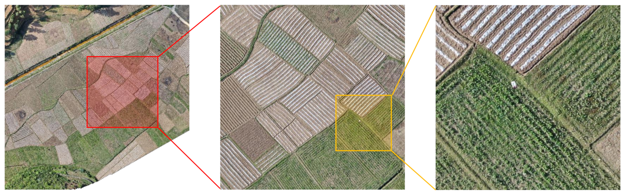
Recently, as a method of image processing, deep learning has been widely used in pixel-level classification (e.g., semantic segmentation) tasks with good results. In particular, the CNN and Transformer based on deep learning methods have attracted more and more attention in crop segmentation tasks due to their excellent performance. To fully realize the potentials of the CNN and Transformer, three problems in agricultural segmentation should be solved. It can be seen from Figure 1, first, that the ultra-high-resolution images need to be cut into small patches because of the memory limitation, which leads to the deficiency of global information and the incomplete structure of the object edge. Second, the crop field and the inside soils are both labeled to the crop category, causing the misclassified prediction of the crop field due to the obvious different characteristics of crop and soils. Third, to obtain the complete image, the patches need to be spliced together, which usually causes edge artifacts and small misclassified objects and holes [5,6]. To cope with the aforementioned three problems and further achieve good segmentation performance, the global context is needed to help the incomplete patches obtain more surrounding information, hence improving the object edge [7]. The local details such as color and texture of the categories are meanwhile needed to help with finer area division. Finally, some well-designed methods are required when restoring the complete images.
The CNN can obtain local information well, but lacks global information caused by the limited receptive field of convolution. FCN [8] and ResNet [9] generate a larger receptive field through continuous stacked convolution layers. Inception [10,11,12,13] and AlexNet [14] obtain more neighborhood information through a larger convolution kernel. DANet [15] and CBAM [16] establish global relations by introducing the attention mechanism. Both methods could obtain global information through the attention mechanism, but this damages the CNN’s original local information, making the acquired global information very limited. Different from CNN-based methods, Transformer can obtain sufficient global information, but lacks local information because of its entirely attention-mechanism-based architecture. ViT [17] is the first visual Transformer to design position encoding, which can supplement the lost position information caused by serialized input. Based on ViT, SETR [18] introduces a CNN decoder and successfully applies Transformer in the semantic segmentation task. ResT [19], VOLO [20], BEIT [21], Swin [22], and CSwin [23] adopt a hierarchical structure similar to the CNN for achieving local information and obtain SOTA performance in many semantic segmentation datasets. It is observed that local information is also very important in the Transformer structure, but the local information generated by the attention module is not as effective as the local feature obtained by the CNN.
According to the aforementioned literature, the CNN lacks global information, but has sufficient local information, and Transformer lacks local information, but has sufficient global information. Therefore, we considered combining the respective advantages of the CNN and Transformer and further propose the Coupled CNN and Transformer Network (CCTNet) to combine the features from the CNN and Transformer branches in this paper. The CCTNet has two independent branches of the CNN and Transformer to retain the advantages of their respective structures. However, it is very difficult to fuse the advantages of the two different architectures. Hence, we propose the Light Adaptive Fusion Module (LAFM) and the Coupled Attention Fusion Module (CAFM) to effectively fuse the features of these two branches. In addition, in order to learn better features of the CNN, Transformer, and the fusion branches, we used three supervised loss functions, respectively. Furthermore, in the inference stage of the model, we propose three methods to improve the performance of the patches, including Overlapping Sliding Window (OSW), Testing Time Augmentation (TTA), and the Post Processing (PP) method of correcting misclassified areas especially for small objects and holes. The code is available at https://github.com/zyxu1996/CCTNet, accessed on 14 April 2022.
To be clearer, the main contributions of this work are summarized as follows:
- We propose the Coupled CNN and Transformer Network (CCTNet) to combine the local modeling advantage of the CNN and the global modeling advantage of Transformer to achieve SOTA performance on the Barley Remote Sensing Dataset.
- The Light Adaptive Fusion Module (LAFM) and the Coupled Attention Fusion Module (CAFM) are proposed to efficiently fuse the dual-branch features of the CNN and Transformer.
- Three methods, namely Overlapping Sliding Window (OSW), Testing Time Augmentation (TTA), and the Post-Processing (PP) method of correcting misclassified areas are introduced to better restore complete crop remote sensing images during the inference stage.
2. Related Work
In this section, some related works regarding State-Of-The-Art (SOTA) remote sensing applications and the model designs are introduced, including CNN-based models, Transformer-based models, and the fusion methods of the CNN and Transformer. These methods provide us with experience in solving global and local information deficiency in crop remote sensing segmentation.
CNN-based models for local information extraction: The conventional FCN [8] model consists of convolution layers and pooling layers, where the convolution operation extracts local features and the pooling operation downsamples the feature size to obtain compact semantic representations. However, it is difficult to obtain semantic representation while preserving local details, since the downsampling operation damages the spatial information [24]. To retrieve the local information, UNet [25] proposes the skip-connection to fuse shallow layers, achieving good performance in the local details. HRNet [26,27] maintains high-resolution representations throughout the process to avoid the deficiency of local information.
To obtain global context information, DeepLab [28,29] and PSPNet [30] propose multi-scale pyramid-based fusion modules to aggregate global context from different receptive fields. Lin et al. proposed FPN [31] to aggregate features of different scales step by step from top to bottom and assign different scale objects to different resolution feature maps. Inspired by the substantial ability of attention mechanisms at modeling global pixels’ relations, DANet [15] designs a dual-attention mechanism of the channel and spatial dimensions to obtain a multi-dimensional global context. HRCNet [32] proposes a lightweight dual-attention module to enhance the global information extraction ability, successfully applying it to the remote sensing image segmentation tasks and achieving SOTA performance.
Despite its advantages in local feature extraction, the ability of the CNN to capture global information is still insufficient, which is very important for crop remote sensing segmentation. Although DeepLab [28,29] and PSPNet [30] expand the receptive field to obtain the multi-scale global context, the global information is still limited to a local region. The attention mechanism provides a good pattern for modeling global information, but is limited by the few module numbers and huge computational burden. Consequently, a pure attention-based lightweight architecture is needed to achieve sufficient global information extraction.
Transformer-based models for global information extraction: Transformer is a pure attention-based architecture with powerful representation capabilities of global relations, but is weak at obtaining local details [33]. Vision Transformer [17] is the first work to apply the Transformer structure to visual tasks by splitting images into patches to meet the input format of Transformer. SETR [18] improved on ViT, applying a CNN decoder to obtain the segmentation results, successfully applying Transformer in semantic segmentation tasks and achieving SOTA performance. Although the ViT architecture explores a feasible way to apply Transformer in visual tasks, it ignores the local representations.
To obtain local representations in the Transformer architecture, ResT [19] designs a patch embedding layer to obtain hierarchical feature representations. VOLO [20], Swin [22], and CSwin [23] adopt a local window attention mechanism to obtain local representations such as the convolution operation. The above methods continuously reach new SOTA performance on the semantic segmentation tasks because of the multi-stage architectures, such as ResNet [9], which are suitable to obtain multi-resolution features [34]. Such architectures provide Transformer with local information, but they are not as good as the CNN. Therefore, the fusion of the CNN and Transformer is intuitively aware and becomes an important research direction.
CNN and Transformer fusion methods: Fusing the CNN and Transformer is intended to combine the superiority of each method, such as the local information extraction ability of the CNN and the global information extraction ability of Transformer. However, it is hard to fuse both superiorities. Therefore, Conformer [35] adopts a parallel structure to exchange features from the local and global branches to maximize the retention of the local and global representations. TransFuse [36] incorporates the multi-level features of the CNN and Transformer via the BiFusion module, so that both the global dependencies and the low-level spatial details can be effectively captured. WiCoNet [37] incorporates a large-scale context branch and a local branch to fuse global and local information, achieving good performance on the BLU, GID, and Potsdam remote sensing datasets. Besides the aforementioned parallel fusion methods, the serial fusion methods can also be used to fuse the CNN and Transformer. Xiao et al. [38] revealed that early convolutions can help Transformers learn better. BoTNet [39] proposes a serial architecture by replacing the spatial convolutions with global self-attention, achieving a strong performance while being highly efficient. CoAtNet [40] is proposed to combine the large model capacity of Transformer and the right inductive bias of the CNN, which achieves the same scores as ViT-huge with 23× fewer data. ConvTransformer [41] was first proposed for video frame sequence learning and video frame synthesis, and it applies a convolutional self-attention layer to encode the sequential dependence and uses a Transformer decoder to capture long-term dependence.
Although the aforementioned fusion methods achieve good performance, there are still some problems: (a) they are trained from scratch; hence, many existing models and pretrained weights cannot be used; (b) this integral architecture will damage the respective characteristics of the CNN and Transformer. To avoid the formerly mentioned deficiencies, we propose a new CNN and Transformer fusion and training method called the CCTNet. The CCTNet fuses the CNN and Transformer branches to generate a new branch, and the three branches are trained with different decoders and loss functions, so that they can keep their respective superiority. In the meantime, the CNN branch and Transformer branch can be flexibly replaced by other better architectures. To achieve better fusion performance, we also employed the LAFM and the CAFM to effectively fuse the local and global features. With the support of the above designs, the CCTNet achieved the best performance on the Barley Remote Sensing Dataset. Table 1 provides a summary of the related work, including the pure CNN methods, the pure Transformer methods, and the CNN and Transformer fusion methods.
3. Methods
This section first introduces the classic CNN model ResNet [9] and the recent Transformer model CSwin Transformer [23]. After that, the framework of Coupled CNN and Transformer Network (CCTNet) is proposed and the CNN and Transformer fusion modules (LAFM and CAFM) are analyzed. Finally, three auxiliary loss functions are designed to improve the performance of the CNN branch, Transformer branch, and fusion branch, respectively. The detailed description of each part is shown below.
3.1. The CNN-Based ResNet
The Residual Network (ResNet) [9] is proposed to solve the degradation of very deep CNN models. It uses the residual connection to connect different convolution layers, so that the feature information from the shallow layers can be propagated to the deep layers. The specific structure of ResNet is shown in Figure 2. Given an input of
(3 represents the RGB channel), the resolution is reduced to after the stem (the combination of convolution, Batch Normalization (BN [11]), Rectified Linear Unit (ReLU), and max pool), where the channel dimension becomes 64. Then, the features pass through four stages to generate the C1, C2, C3, and C4 features. The resolutions of the four features are successively reduced by half, respectively , , , and , and the channels sequentially increase to C, 2C, 4C, and 8C. Each stage contains several residual blocks (also called ResNet blocks); the input feature is added to the main branch output feature via a shortcut, followed by a ReLU activation function to enhance the non-linearity of the model. At the first block of each stage, there will be a downsampling convolution and BN in the residual connection to downsample the features. The design of bottleneck architectures and residual connections makes the training process easier. To adjust the channel dimensions and block numbers of ResNet, we could obtain four model sizes named ResNet-18, ResNet-34, ResNet-50, and ResNet-101. Figure 2 displays the ResNet-50 model with 3, 4, 6, and 3 blocks in each stage. ResNet was chosen as the CNN branch because it is easy to scale to different model sizes for different task requirements. Furthermore, the multi-scale output features of C1, C2, C3, and C4 are suitable for dealing with multi-scale objects.
3.2. Basic CSwin Transformer
The structure of CSwin Transformer [23] is shown in Figure 3. First, through convolution token embedding (the convolution kernel is , and the stride is 4), the input of (3 represents the RGB channel) is divided into windows of size , for extracting the local features and location information of each window, then mapping Channel 3 to C. The CSwin Transformer block consists of Layer Normalization (LN), Cross-Shaped Window Self-Attention (CSWSA), and Multilayer Perceptron (MLP). LN normalizes the features to make the training process more stable; CSWSA is used to calculate the attention relation between pixels; MLP contains a large number of learnable parameters for recording the learned relation coefficient. After the CSwin Transformer block extracting global information, then the convolution with stride 2 (Conv S2) will downsample the features to half and expand the channels to double. For example, after the Conv S2 behind Stage1, the shape of the feature is changed from to . Each Stage outputs features T1, T2, T3, and T4 in turn, with resolutions of , , , and and channels of C, 2C, 4C, and 8C. These features contain information at different scales and can be well adapted to downstream semantic segmentation tasks. By adjusting the number of blocks in each stage, four scales of CSwin Transformer [23] can be formed, namely CSwin-Tiny, CSwin-Small, CSwin-Base, and CSwin-Large, and the feature extraction capability is improved in turn. CSwin Transformer is proven to be powerful and efficient, and the multi-scale outputs can also meet the segmentation task requirements; hence, it was chosen as the Transformer branch.
To explain the special design of CSWSA, the commonly used full self-attention is shown in Figure 4a. To obtain the contextual relationship of this red pixel, it is necessary to calculate the attention relations of the entire image, so the computational complexity is the quadratic complexity of the input image size. However, in Figure 4b, CSWSA adopts a special self-attention design, which splits a cross area into two strip-shaped areas in the horizontal and vertical directions and controls the width of the strip by adjusting the value of SW. Self-attention is calculated in each of these two strip areas, and the positional information is encoded by Locally Enhanced Positional Encoding (LEPE, a convolution). The features enhanced by LEPE are added to the generated attention features through a residual connection. After that, the Concat operation concatenates the results in the horizontal and vertical directions to generate cross-shaped attention features. Compared to full self-attention, the cross-shaped attention design reduces the computational costs and the LEPE enhances the local information, which shows that CSWSA is a more efficient design.
3.3. Framework of the Proposed CCTNet
As shown in Figure 5, the CCTNet is divided into four parts, namely the CNN branch, Transformer branch, fusion module, and loss function. The CNN branch generates four features C1, C2, C3, and C4, where the resolutions are , , , and of the input resolution, respectively. The number of channels increases in multiples in turn. The Transformer branch generates four features T1, T2, T3, and T4. The resolution is the same as the CNN, and the channel numbers are also doubled. The CNN branch contains richer local information, and the Transformer branch contains more global information. After obtaining the C and T features, first, the LAFM is used to fuse the features of C1 and T1 and C2 and T2, because the LAFM can reassign weights to the fused features while preserving the local information of the CNN branch and the global information of the Transformer branch to the greatest extent. Moreover, the LAFM is a lightweight design; hence, it is applied in shallow features without any burden. The CAFM is a feature reconstruction module based on the attention mechanism, which can select the favorable information from the CNN to supplement Transformer, as well as select the favorable information from Transformer to supplement the CNN. Then, the CAFM fuses the features of C3 and T3 and C4 and T4. The mutual promotion helps the fused CT1, CT2, CT3, and CT4 features to concurrently gain the advantages of the CNN and Transformer branches. Finally, two auxiliary loss functions (LossC and LossT) are used to supervise the CNN and Transformer branches, so that both branches can learn good feature representations, thereby improving the fused features.
For the fusion branch, we adopted an auxiliary loss (LossCT3) to supervise the feature learning of CT3 and another main loss function (LossCT) to supervise the feature learning of CT1, CT2, CT3, and CT4. As displayed in Figure 6, the decoders of LossC, LossT, and LossCT are Multi-Scale Fusion decoders (MSF decoders) with four resolution inputs; the decoder of LossCT3 is a Single-Scale decoder (SS decoder) with input CT3.
3.4. Two Designs for the CNN and Transformer Fusion Module
Two modules, the Light Adaptive Fusion Module (LAFM) and the Couple Attention Fusion Module (CAFM), are proposed to solve the challenging feature fusion problems. The LAFM learns the feature weights of the CNN and Transformer and assigns larger weights to the local features of the CNN and the global features of Transformer, while suppressing other unimportant features. The CAFM uses the attention mechanism to learn the favorable feature information of the CNN and Transformer. For example, the CNN can obtain the global information supplement from Transformer, and Transformer can obtain the local information supplement from the CNN.
3.4.1. Light Adaptive Fusion Module
As can be seen in Figure 7, first, the input features of the CNN (C1, C2) and Transformer (T1, T2) go through a convolution, respectively. Next, the Concat operation merges the two features and sends them to the next convolution to make the interaction among the CNN and Transformer features. Then, the features are separated by the split operation, followed by a convolution and a Sigmoid function, respectively, to normalize the pixel values from 0 to 1 to avoid the maximum and minimum. Finally, the stack operation to parallel connect both features in the channel dimension is used, and the softmax function is applied to obtain the pixel-level weights. The weights of the CNN and Transformer in the same pixel position are summed to 1. The generated feature weight maps of the CNN and Transformer are then multiplied pixel by pixel with the previous features to perform pixel-level reweighting operations. In addition, we used the residual connection (the dotted line) to add previous features to accelerate model optimization and reduce the learning difficulty of feature weight maps.
The feature weight maps learned by the CNN and Transformer are shown in Figure 8. The ground truth means the true value; it is obtained by manual annotation. All the remote sensing images in this paper have corresponding ground truths. The larger weights are more red; the smaller weights are more blue; the weights of CNN and transformer at the same pixel are added to 1; hence they are the inverse of each other. Observing Figure 8, we can see that the CNN usually has more red and larger weights at the edge details and Transformer usually has larger weights on larger objects, which also proves the respective advantages of the CNN and Transformer in processing local and global information.
3.4.2. Coupled Attention Fusion Module
The CAFM consists of a basic attention module, as well as a global and local interaction module. As displayed in Figure 9, the inputs of the attention module are the CNN and Transformer features, where x and y can be C and T or T and C, respectively. First, x goes through a convolution to generate the query and y goes through two convolution to generate the key and value. Then, using the transpose of the query matrix and the key to perform matrix multiplication to generate the attention map, the softmax function then normalizes the attention map. The attention map represents the contribution of each pixel in the key to each pixel in the query. Finally, the transposed value is matrix multiplied by the attention map to generate the reweighting features. In general, the whole process is to help y reweight features via the information of x. Therefore, when x comes from Transformer (T3 or T4) and y comes from CNN (C3 or C4), the global information of Transformer is introduced to reweight the local features of the CNN, which we call global to local. Correspondingly, when x comes from the CNN (C3 or C4) and y comes from Transformer (T3 or T4), the local information of the CNN is introduced to reweight the global features of Transformer, which is called local to global. Finally, after the two processes of global to local and local to global, the CNN features fused with global information and the Transformer features fused with local information can be obtained. Concatenating the above two features and applying a convolution to obtain the final output CT3 or CT4, the above processes establish a good connection between the CNN and Transformer, and the interactive fusion of local and global information promotes the optimization of their respective branches.
3.5. Loss Functions’ Design
The loss function is significant in model optimization, determining the final segmentation effect in the semantic segmentation task. The commonly used loss function is the cross-entropy loss function, which is defined in Formula (1), where N indicates the number of classification categories, p(xi) ∈ {0, 1} is the ground truth of pixel x belonging to category i, and q(xi) ∈ [0, 1] represents the probability that the pixel x is predicted as category i. To calculate the loss of the entire pixels in an image, we sum the loss of the pixels and average them.
The loss functions used in this paper are all cross-entropy loss functions, including a main loss function and three auxiliary loss functions. These are respectively the main loss function of the fusion branch (LossCT), the auxiliary loss function of the fusion branch (LossCTAux), the auxiliary loss function of the CNN branch (LossC), and the auxiliary loss function of the Transformer branch (LossT). Among them, LossC and LossT are both used to supervise the optimization process of the CNN and Transformer branches; removing them will not affect the normal training process. LossCTAux is used to enhance the feature CT3. LossCT is the most important loss function, which directly determines whether the model can be trained and optimized normally. The final loss function (LossAll) of the entire model can be expressed by Formula (2):
4. Experimental Results
In this section, we first explore the performance of the mainstream CNN and Transformer models on the Barley Remote Sensing Dataset and select the best-performing Transformer model CSwin-Tiny and the most widely used CNN model ResNet-50 as benchmarks to explore the fusion method of the CNN and Transformer. Then, we study the effects of the fusion modules, the LAFM and CAFM, as well as the auxiliary loss functions. Finally, we discuss the combination of different model sizes of the CNN and Transformer to verify the flexibility of our proposed CCTNet.
4.1. Dataset and Experimental Settings
The Barley Remote Sensing Dataset (https://tianchi.aliyun.com/dataset/dataDetail?dataId=74952, accessed on 28 February 2022) presents a rural area in Xingren City, Guizhou Province, China, containing a large amount of crop fields. It was collected by an Unmanned Aerial Vehicle (UAV) near the ground, including the three spectrum bands of red, green, and blue. It collected data on crops such as cured tobacco, corn, and barley rice and provides a data basis for crop classification and yield prediction. The dataset is shown in Figure 10, which contains two ultra-high-resolution images, image_1 and image_2, with resolutions of pixels and pixels, respectively. A total of four categories including background (white), cured tobacco (green), corn (yellow), and barley rice (red) are labeled as Classes 0, 1, 2, and 3. Except for the above four categories, the rest of the picture is transparent. The background category mainly includes buildings, vegetation, and other unimportant crops. The three crops of cured tobacco, corn, and barley are divided by region, and the soil inside the crop field is also labeled as the corresponding crop category. The crop fields are not all regular, but the same crops are more likely to be distributed in the same area.
As can be seen from Figure 10, the ground truth, the category distributions of the two images are inconsistent. In image_1, cured tobacco and barley rice take the larger proportion and corn takes a small proportion, but in image_2, corn and barley rice take the larger proportion and cured tobacco takes a small proportion. This situation will affect the training of the model, leading to low performance. Therefore, we divided the training set and test set after cutting the two images into many patches, each of which is pixels, as shown in Figure 10. The training region and test region were interval-sampled, and the completely transparent parts were discarded. Finally, we obtained 44 samples for training and 41 samples for testing. It is worth noting that for the rest with a resolution smaller than pixels, we reversed the direction to cut a area; see the rightmost column and the bottom row in image_1 and image_2. In fact, due to memory limitations, the obtained images with a resolution of pixels could not be directly used for training and testing, and further processing was required. In Figure 11, we use a sliding window [32,42] with overlap to select training and testing data online, as well as to discard the completely transparent parts. Finally, the patches were restored to , and then, all the patches were spliced to obtain image_1 and image_2 with original resolutions of pixels and pixels.
The dataset division details, experimental platform, and training settings are listed in Table 2, where TrS, TeS, DL, CE, and LR denote Training Size, Testing Size, Cross-Entropy, Deep Learning, and Learning Rate, respectively. The evaluating metrics follow the official advice, including Precision, Recall, F1, Overall Accuracy (OA) and mean Intersection over Union (mIoU). The formula is shown in Formulae (3) and (4). The AdamW optimizer was used to accelerate the training process. The Poly learning rate scheduler was applied to make the training process smoother. The CE loss function is the commonly used segmentation loss function to calculate errors between the prediction and ground truth. LR, mini-batch size, and epoch were manually adjusted according to the evaluation results.
where T, F, P, and N represent true, false, positive, and negative, respectively. TP denotes the pixels of the truly predicted positive class. TN is the truly predicted negative pixels. FP is the falsely predicted positive pixels. FN is the falsely predicted negative pixels. mIoU is the average of all categories of the IoU. Among the formerly mentioned metrics, F1, OA, and mIoU are the main reference indicators.
4.2. Methods’ Comparison on the Barley Remote Sensing Dataset
This part first explores the performance of the classic CNN and the latest Transformer models on the Barley Remote Sensing Dataset, including BiseNet-V2 [43], FCN [8], UNet [25], FPN [31], DANet [15], ResNet-50* [9] (* means the segmentation application of ResNet), PSPNet [30], and DeepLab-V3 [28]. It is worth noting that DANet [15], PSPNet [30], and DeepLab-V3 [28] all use dilated ResNet-50 as the backbone, which uses dilated convolution to replace downsampling convolution to keep high-resolution representations. FPN and ResNet-50* are based on the original ResNet-50 backbone, using an MSF decoder. The Transformer-based models all use a multi-stage structure like ResNet-50* to fuse multi-scale features, which can better fuse local details and deep semantic information.
The experimental results are shown in Table 3. Taking the mIoU as the main comparison indicator, it can be seen that BiseNet-V2 [43] and FCN [8], which are stacked with simple convolutions, achieved 62.18% and 64.51% accuracy, respectively. Using the encoder–decoder method of UNet [25] to fuse shallow features, the result achieved a 0.32% improvement compared to FCN. By introducing the attention mechanism or incorporating multi-scale features, FPN, DANet, ResNet-50*, PSPNet, and DeepLab-V3 had mIoU scores close to 70%. We can conclude that the attention mechanism and multi-scale fusion methods can significantly improve the segmentation performance, which benefits from the promotion of global information and local information. Transformer models that use multi-scale feature fusion, such as ResT-Tiny [19], Swin-Tiny [22], and VOLO-D1 [20], obtained good mIoU scores, but were slightly weaker than the CNN models. However, CSwin-Tiny [23] using Locally Enhanced Positional Encoding (LEPE) significantly outperformed other Transformer models. As the Transformer model lacks local information, the LEPE enhances CSwin-Tiny’s ability to extract local features, which shows the significance of local information.
Finally, in order to pursue the best performance while considering the flexibility of the model size, we adopted the best-performing CSwin as the Transformer benchmark and the flexible ResNet as the CNN benchmark. CSwin provides four model sizes of Tiny, Small, Base, and Large, and ResNet includes four model sizes of ResNet-18, ResNet-34, ResNet-50, and ResNet-101. The subsequent experiments were based on the Transformer branch of CSwin-Tiny and the CNN branch of ResNet-50, and the decoder adopts the MSF decoder in Figure 5. The experimental settings followed those in Table 2.
4.3. Study of the CNN and Transformer Fusion Modules
Because of the huge diversity of the CNN and Transformer features, the simple strategy to directly merge these two features will be a big challenge, resulting in a bad performance. Existing methods, such as Conformer [35] and TransFuse [36], fuse the CNN and Transformer at the shallow level and send the fused features in the subsequent training of the CNN and Transformer branches. Such a method confuses the characteristics of the CNN and Transformer, making their respective advantages fade out. Therefore, we propose the Light Adaptive Fusion Module (LAFM) and the Coupled Attention Fusion Module (CAFM) to fuse features without damaging their diversity. In this section, the location settings of the LAFM and CAFM at four positions to generate CT1, CT2, CT3, and CT4 are discussed in the experiments. The four positions are respectively behind the four stages in the CNN and Transformer branches, making the fusion of the CNN and Transformer features. Moreover, some detailed designs of the structure are also discussed.
4.3.1. The Location Settings of the LAFM and the CAFM
To generate the four fused features CT1, CT2, CT3, and CT4, four fusion modules at the corresponding positions are selected from the LAFM or the CAFM. ①, ②, ③, and ④ represent the positions to generate CT1, CT2, CT3, and CT4 respectively. “∖” means that the marked module was not used. Taking the mIoU as the main reference indicator, the first line in Table 4 represents that without fusion modules, the score was lower than using only CSwin-tiny, which can only reach 71.12%. This shows that simply fusing the features of the CNN and Transformer cannot obtain their respective advantages, but results in being worse. The second line uses the LAFM to replace the original rough fusion method, and the mIoU increased by 0.36%, proving the effectiveness of the LAFM. The third and fourth lines replace the two positions ③ or ④ with the CAFM, which further improved the performance. When both positions ③ and ④ are replaced by the CAFM, the best mIoU score of 72.07% was obtained, which was 0.59% higher than the second experiment, indicating that the CAFM is effective and the effect is better than the LAFM.
However, the effect of the CAFM is related to the position. For example, being set in the ②④ positions, the score was not as good as that in the ④ position as the CAFM is an attention module that usually works better on rich semantic features, such as positions ③ and ④. Moreover, the CAFM numbers were exquisite; the positions ②③④ all use the CAFM, but obtained poor performance. When the CAFM is placed in the ① or ② position, it took up much memory. Consequently, the LAFM is more lightweight and is suitable for the positions ① and ②; the CAFM has better performance, but has a large computational burden; it is suitable for the positions 3 and 4 to fuse rich semantic features.
4.3.2. The Structure Settings of the LAFM and the CAFM
To make the LAFM and the CAFM work, some special structural designs are required. The LAFM includes the residual connection to fuse shallow layers and accelerate the model convergence. The CAFM consists of two major parts, the global to local (G → L) module and the local to global (L → G) module, to generate two fusion features. After obtaining the two fusion features, there are two methods (Concat and add) to fuse them. The Concat operation splices the two features in the channel dimension, and it can better retain the original information. The add operation fuses the two features in an elementwise sum way, which may confuse the information of local and global. Here, we performed an ablation study (see Table 5) by adding or removing the residual connection in the LAFM. Furthermore, the choices of the G → L and L → G modules are discussed, and the fusion methods of Concat and add were tried when fusing the G → L and L → G modules in the CAFM.
Table 5 shows the experimental results. Taking the mIoU as the main reference, the analysis is given below. First, looking at the top three lines, when only G → L or L → G is used, the mIoU was 71.38% and 71.55%, respectively, which is a significant drop compared to the 72.07% score obtained by using the two modules simultaneously. This shows that the CNN and Transformer can complement each other to improve the performance. The fourth line replaces the Fusion mode with add, and the mIoU had a big decrease of 0.85%, indicating that the Concat fusion method is significantly better than add. The fifth line removes the residual connection in the LAFM, and the mIoU was also reduced by 0.55%, proving that the residual structure is significant in the LAFM. Through the exploration of the structure designs, we finally determined the appropriate structure settings for the LAFM and the CAFM and achieved good performance.
4.4. Ablation Experiments of the Auxiliary Loss Function
The auxiliary loss function plays a vital role in learning more effective representations in semantic segmentation tasks. It works in the training stage and can be completely discarded when performing inferring, so it is free on the inference consumption. A total of three auxiliary loss functions were used in this paper, where Aux Loss CT3 was applied to supervise the feature CT3 and Aux Loss C and T were used to optimize the CNN and Transformer branches. In Table 6, we discuss the experimental settings with (w/) or without (w/o) these auxiliary loss functions and the situation of Aux Loss C and T sharing the same decoder. The detailed analysis is as follows:
The experiment in the first line removed Aux Loss C and T; compared with the second line, the mIoU score decreased by 0.82%. Without the extra supervision of Aux Loss C and T, the model generated poor features of the CNN and Transformer branches. Moreover, the auxiliary loss functions can also synchronize the learning progress of the CNN and Transformer, achieving the coupled optimization. The third experiment shared the same parameters in the decoder, resulting in the mIoU dropping sharply. Because the diversity of the CNN and Transformer is tremendous, the same decoder parameters cannot afford the CNN and Transformer at the same time. The last experiment removed Aux Loss CT3, and the mIoU had a slight drop of 0.31%. The purpose of Aux Loss CT3 is to make CT3 learn better features, so that the next CT4 can also learn good features. Therefore, in the semantic segmentation task, it is common and effective to add an auxiliary loss function at the third output feature of the encoder. Consequently, auxiliary loss functions are very important in the fusion process of the CNN and Transformer, especially the CCTNet proposed in this paper, which relies on the independent and good features of the CNN and Transformer. Of course, we can also train the CNN and Transformer branches separately and then fix the weights; this will keep their respective characteristics. However, this practice increases the complexity of the model design; it is not an end-to-end architecture like our proposed CCTNet.
4.5. Results of Different CNN and Transformer Model Sizes
Because of the independent design of the CNN and Transformer branches, the CCTNet makes it easy to adjust the size of the CNN and Transformer models, meaning that the pretrained weights can be used to make it easier to fit in different downstream tasks. This section discusses the combinations of different CNN and Transformer model sizes for the Barley Remote Sensing Dataset in Table 7. The CNN was selected from ResNet-18, ResNet-34, ResNet-50, and ResNet-101, where the larger number means a larger size. Transformer was selected from CSwin-Tiny, CSwin-Small, and CSwin-Base; the model size increases in turn.
Fixing Transformer to CSwin-Tiny, the mIoU gradually increased when the model size changed from ResNet-18 to ResNet-50, but the mIoU of ResNet-101 had a slight decrease, indicating that changing the model size of the CNN will significantly affect the performance. When the CNN branch was ResNet-50, the accuracy saturated. Therefore, we fixed the CNN to ResNet-50 and changed the Transformer size; the mIoU had a small decline. It can be seen that the Transformer size did not affect the final accuracy very much, and CSwin-Tiny can already meet the needs of the CCTNet for global information. Furthermore, the Transformer branch had the main computation consumption, so using the lightweight Transformer model in this paper is better.
4.6. Study on the Improvements of Each Category
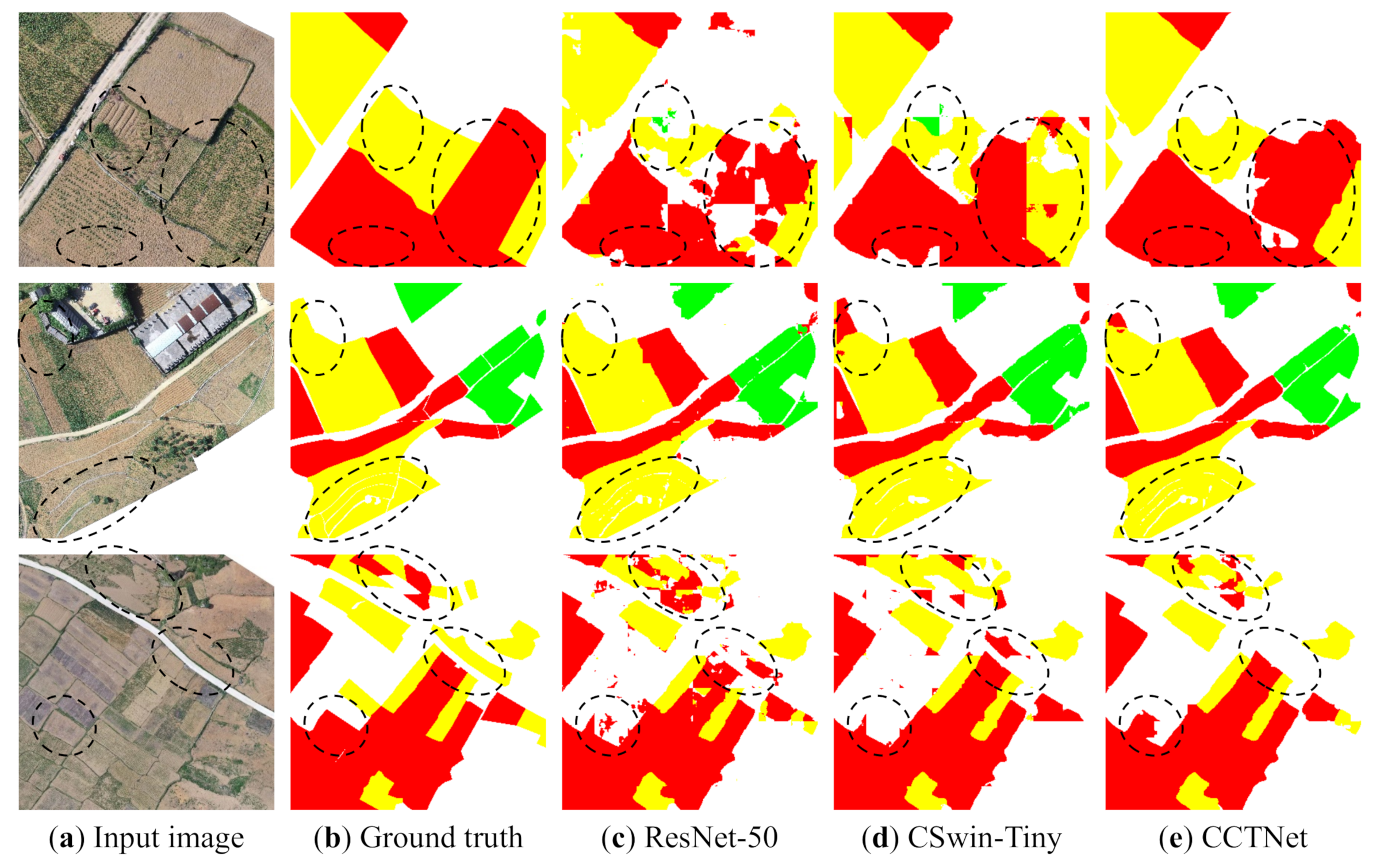
In this section, we compare the performance of ResNet-50* [9], CSwin-Tiny [23], and CCTNet on the mIoU performance of four categories: background, cured tobacco, corn, and barley rice. It can be seen in Table 8 that the Transformer method was more effective, because the Transformer-based method CSwin-Tiny was 0.25%, 0.48%, 1.57%, and 1.91% higher than the CNN-based method ResNet-50* in the above four categories, especially on the corn and barley rice categories. The reason is that the background and cured tobacco categories are concentrated in continuous regions without too much interference, and the background is easier to recognize, so both the CNN and Transformer classified correctly more easily. However, the corn and barley rice categories were scattered, and these two categories appear alternately and interfere with each other. Therefore, the global context is needed here, and Transformer performed better in the corn and barley rice categories. Compared with ResNet-50*, the CCTNet achieved a 1.00%, 1.28%, 2.48%, and 2.81% IoU promotion, respectively, as well as performed greatly in the corn and barley rice categories, indicating that the CCTNet has the advantages of the Transformer structure. Compared with CSwin-Tiny, the CCTNet increased the IoU scores by 0.75%, 0.80%, 0.91%, and 0.90%, respectively, which benefited from the introduction of the CNN for improving the segmentation in edge details. Meanwhile, we analyzed the inference speed of each model; the unit was the processed images per second (img/s). It can be seen that the CCTNet only obtained a slight inference speed decrease, which shows that the increment of the mIoU score was not obtained at the expense of significantly increasing the execution time.
In Figure 12, we compare the prediction maps of ResNet-50* [9], CSwin-Tiny [23], and the CCTNet on the local details and global classification. It can be seen that the CCTNet performed better on edge and detail processing than CSwin-Tiny and performed better on global classification than ResNet-50*. This shows that the CCTNet successfully combines the advantages of CNN in local modeling and Transformer in global modeling and achieved good results in the crop remote sensing segmentation task.
5. Discussion
Some methods for improving model performance at inference time were introduced here, including the Overlapping Sliding Window testing (OSW), Testing Time Augmentation (TTA), and Post-Processing (PP) methods to remove small objects and small holes. Due to the large image resolution and memory limitations, we cut the image into pieces before running the model, resulting in incomplete objects at the slit and affecting the segmentation effect [44]. Therefore, the OSW method was introduced. It retained a overlap during inference, so that the overlapped part was inside the image, thus reducing the influence of incomplete objects. TTA is a method to fuse different predictions by translating different inputs, by averaging the results to obtain better performance. In this paper, horizontal flipping and vertical flipping were used to generate different inputs in TTA. Moreover, we observed that the category regions in the Barley Remote Sensing Dataset were mainly large; small areas are very rare in this dataset. Therefore, we specifically proposed a post-processing method to remove small objects and small holes. The specific process was as follows: first, calculate the number of pixels in a connected area, then set a threshold (40,000 pixels in this paper) for the maximum pixels in the connected area; finally, replace the objects or holes smaller than the threshold with surrounding pixels.
Table 9 and Figure 13 display the improvements of using the above three methods. Without OSW, the gap of the patch had obvious edge artifacts. When using OSW, the edge parts were significantly improved, and the mIoU increased by 0.47%, which shows the availability of OSW for improving the edge parts. When using TTA, the mIoU further increased by 0.16%, but there were still some small wrongly predicted regions and holes. When PP was used, the mIoU increased by 0.27%; these mispredicted parts were replaced with surrounding categories, making them look cleaner and more complete. Compared with the insignificant mIoU promotion, the visual effects are more important.
6. Conclusions
In this paper, we analyzed challenging problems in crop remote sensing images’ segmentation, such as incomplete objects at the edge and the imbalance of global and local information, which severely damage the performance. To solve the above problems, the proposed model should combine the advantages of CNN in local modeling and Transformer in global modeling. Therefore, we proposed the CCTNet to fuse the features of the CNN and Transformer branches, while keeping their respective advantages. Furthermore, to conduct end-to-end training of the CCTNet, the auxiliary loss functions were proposed to supervise the optimization process. In order to smoothly fuse the features of the CNN and Transformer, we proposed the LAFM and the CAFM to selectively fuse their advantages while ignoring their drawbacks. By using the above methods, our CCTNet achieved a 1.89% mIoU improvement compared to the CNN benchmark ResNet-50* and a 0.84% mIoU promotion compared to the Transformer benchmark CSwin-Tiny. This proves the importance of combining the CNN and Transformer for the crop segmentation task. In addition, three methods were introduced to further improve the performance at inference time, for example using the overlapping slide window to eliminate edge artifacts, applying the testing time augmentation method to enhance the stability, and employing the post-processing method to remove small objects and holes to obtain clear and complete prediction maps. The application of the above three methods further brought a 0.9% increase in the mIoU, finally achieving 72.97% mIoU scores on the Barley Remote Sensing Dataset. The ability of the current CCTNet may be limited, but based on the flexibility of the structure, it can be continuously optimized with the development of the CNN and Transformer methods. In the future, we will consider introducing multi-spectral crop data to improve the classification of the challenging corn and barley rice categories.
Author Contributions
H.W., Z.X. and J.L. conceived of the idea; Z.X. verified the idea and designed the study; X.C. and J.L. analyzed the experimental results; Z.X. and T.Z. wrote the paper; H.W. and T.Z. gave comments on and suggestions for the manuscript. All authors read and approved the submitted manuscript.
Funding
This work was supported by the Fundamental Research Funds for the China Central Universities of USTB (FRF-DF-19-002) and the Scientific and Technological Innovation Foundation of Shunde Graduate School, USTB (BK20BE014).
Institutional Review Board Statement
Not applicable.
Informed Consent Statement
Not applicable.
Data Availability Statement
Not applicable.
Acknowledgments
The authors thank Guangzhou Jingwei Information Technology Co., Ltd., and the Xingren City government for providing the Barley Remote Sensing Dataset.
Conflicts of Interest
The authors declare no conflict of interest.
References
- Witharana, C.; Bhuiyan, M.A.E.; Liljedahl, A.K.; Kanevskiy, M.; Epstein, H.E.; Jones, B.M.; Daanen, R.; Griffin, C.G.; Kent, K.; Jones, M.K.W. Understanding the synergies of deep learning and data fusion of multispectral and panchromatic high resolution commercial satellite imagery for automated ice-wedge polygon detection. ISPRS J. Photogramm. Remote Sens. 2020, 170, 174–191. [Google Scholar] [CrossRef]
- Zhang, T.; Su, J.; Liu, C.; Chen, W.H. State and parameter estimation of the AquaCrop model for winter wheat using sensitivity informed particle filter. Comput. Electron. Agric. 2021, 180, 105909. [Google Scholar] [CrossRef]
- Zhang, T.; Su, J.; Xu, Z.; Luo, Y.; Li, J. Sentinel-2 satellite imagery for urban land cover classification by optimized random forest classifier. Appl. Sci. 2021, 11, 543. [Google Scholar] [CrossRef]
- Tilman, D.; Balzer, C.; Hill, J.; Befort, B.L. Global food demand and the sustainable intensification of agriculture. Proc. Natl. Acad. Sci. USA 2011, 108, 20260–20264. [Google Scholar] [CrossRef] [PubMed] [Green Version]
- Qin, X.; Zhang, Z.; Huang, C.; Gao, C.; Dehghan, M.; Jagersand, M. Basnet: Boundary-aware salient object detection. In Proceedings of the IEEE Conference on Computer Vision and Pattern Recognition, Long Beach, CA, USA, 16–20 June 2019; pp. 7479–7489. [Google Scholar]
- Yang, G.; Zhang, Q.; Zhang, G. EANet: Edge-Aware Network for the Extraction of Buildings from Aerial Images. Remote Sens. 2020, 12, 2161. [Google Scholar] [CrossRef]
- Zhen, M.; Wang, J.; Zhou, L.; Li, S.; Shen, T.; Shang, J.; Fang, T.; Quan, L. Joint Semantic Segmentation and Boundary Detection using Iterative Pyramid Contexts. In Proceedings of the IEEE/CVF Conference on Computer Vision and Pattern Recognition, Seattle, WA, USA, 14–19 June 2020; pp. 13666–13675. [Google Scholar]
- Long, J.; Shelhamer, E.; Darrell, T. Fully convolutional networks for semantic segmentation. In Proceedings of the IEEE Conference on Computer Vision and Pattern Recognition, Boston, MA, USA, 7–12 June 2015; pp. 3431–3440. [Google Scholar]
- He, K.; Zhang, X.; Ren, S.; Sun, J. Deep residual learning for image recognition. In Proceedings of the IEEE Conference on Computer Vision and Pattern Recognition, Las Vegas, NV, USA, 27–30 June 2016; pp. 770–778. [Google Scholar]
- Szegedy, C.; Liu, W.; Jia, Y.; Sermanet, P.; Reed, S.; Anguelov, D.; Erhan, D.; Vanhoucke, V.; Rabinovich, A. Going deeper with convolutions. In Proceedings of the IEEE Conference on Computer Vision and Pattern Recognition, Boston, MA, USA, 7–12 June 2015; pp. 1–9. [Google Scholar]
- Ioffe, S.; Szegedy, C. Batch normalization: Accelerating deep network training by reducing internal covariate shift. In Proceedings of the International Conference on Machine Learning, PMLR, Lille, France, 6–11 July 2015; pp. 448–456. [Google Scholar]
- Szegedy, C.; Vanhoucke, V.; Ioffe, S.; Shlens, J.; Wojna, Z. Rethinking the inception architecture for computer vision. In Proceedings of the IEEE Conference on Computer Vision and Pattern Recognition, Las Vegas, NV, USA, 27–30 June 2016; pp. 2818–2826. [Google Scholar]
- Szegedy, C.; Ioffe, S.; Vanhoucke, V.; Alemi, A.A. Inception-v4, inception-resnet and the impact of residual connections on learning. In Proceedings of the Thirty-First AAAI Conference on Artificial Intelligence, San Francisco, CA, USA, 4–9 February 2017; Volume 31. [Google Scholar]
- Krizhevsky, A.; Sutskever, I.; Hinton, G.E. Imagenet classification with deep convolutional neural networks. Adv. Neural Inf. Process. Syst. 2012, 25, 1097–1105. [Google Scholar] [CrossRef]
- Fu, J.; Liu, J.; Tian, H.; Li, Y.; Bao, Y.; Fang, Z.; Lu, H. Dual attention network for scene segmentation. In Proceedings of the IEEE Conference on Computer Vision and Pattern Recognition, Long Beach, CA, USA, 16–20 June 2019; pp. 3146–3154. [Google Scholar]
- Woo, S.; Park, J.; Lee, J.Y.; Kweon, I.S. Cbam: Convolutional block attention module. In Proceedings of the European Conference on Computer Vision (ECCV), Munich, Germany, 8–14 September 2018; pp. 3–19. [Google Scholar]
- Dosovitskiy, A.; Beyer, L.; Kolesnikov, A.; Weissenborn, D.; Zhai, X.; Unterthiner, T.; Dehghani, M.; Minderer, M.; Heigold, G.; Gelly, S.; et al. An image is worth 16x16 words: Transformers for image recognition at scale. arXiv 2020, arXiv:2010.11929. [Google Scholar]
- Zheng, S.; Lu, J.; Zhao, H.; Zhu, X.; Luo, Z.; Wang, Y.; Fu, Y.; Feng, J.; Xiang, T.; Torr, P.H.S.; et al. Rethinking Semantic Segmentation from a Sequence-to-Sequence Perspective with Transformers. In Proceedings of the 2021 IEEE/CVF Conference on Computer Vision and Pattern Recognition (CVPR), Nashville, TN, USA, 20–25 June 2021; pp. 6877–6886. [Google Scholar]
- Zhang, Q.; Yang, Y. ResT: An Efficient Transformer for Visual Recognition. arXiv 2021, arXiv:2105.13677. [Google Scholar]
- Yuan, L.; Hou, Q.; Jiang, Z.; Feng, J.; Yan, S. VOLO: Vision Outlooker for Visual Recognition. arXiv 2021, arXiv:abs/2106.13112. [Google Scholar]
- Bao, H.; Dong, L.; Wei, F. BEiT: BERT Pre-Training of Image Transformers. arXiv 2021, arXiv:abs/2106.08254. [Google Scholar]
- Liu, Z.; Lin, Y.; Cao, Y.; Hu, H.; Wei, Y.; Zhang, Z.; Lin, S.; Guo, B. Swin transformer: Hierarchical vision transformer using shifted windows. arXiv 2021, arXiv:2103.14030. [Google Scholar]
- Dong, X.; Bao, J.; Chen, D.; Zhang, W.; Yu, N.; Yuan, L.; Chen, D.; Guo, B. CSWin Transformer: A General Vision Transformer Backbone with Cross-Shaped Windows. arXiv 2021, arXiv:abs/2107.00652. [Google Scholar]
- Ling, Z.; Zhang, A.; Ma, D.; Shi, Y.; Wen, H. Deep Siamese Semantic Segmentation Network for PCB Welding Defect Detection. IEEE Trans. Instrum. Meas. 2022, 71, 5006511. [Google Scholar] [CrossRef]
- Ronneberger, O.; Fischer, P.; Brox, T. U-net: Convolutional Networks for Biomedical Image Segmentation. In Proceedings of the International Conference on Medical Image Computing And Computer-Assisted Intervention, Munich, Germany, 5–9 October 2015; pp. 234–241. [Google Scholar]
- Sun, K.; Xiao, B.; Liu, D.; Wang, J. Deep high-resolution representation learning for human pose estimation. In Proceedings of the IEEE Conference on Computer Vision and Pattern Recognition, Long Beach, CA, USA, 16–20 June 2019; pp. 5693–5703. [Google Scholar]
- Sun, K.; Zhao, Y.; Jiang, B.; Cheng, T.; Xiao, B.; Liu, D.; Mu, Y.; Wang, X.; Liu, W.; Wang, J. High-resolution representations for labeling pixels and regions. arXiv 2019, arXiv:1904.04514. [Google Scholar]
- Chen, L.C.; Papandreou, G.; Schroff, F.; Adam, H. Rethinking atrous convolution for semantic image segmentation. arXiv 2017, arXiv:1706.05587. [Google Scholar]
- Chen, L.C.; Zhu, Y.; Papandreou, G.; Schroff, F.; Adam, H. Encoder-decoder with atrous separable convolution for semantic image segmentation. In Proceedings of the European Conference on Computer Vision (ECCV), Munich, Germany, 8–14 September 2018; pp. 801–818. [Google Scholar]
- Zhao, H.; Shi, J.; Qi, X.; Wang, X.; Jia, J. Pyramid scene parsing network. In Proceedings of the IEEE Conference on Computer Vision and Pattern Recognition, Honolulu, HI, USA, 21–26 July 2017; pp. 2881–2890. [Google Scholar]
- Lin, T.Y.; Dollár, P.; Girshick, R.; He, K.; Hariharan, B.; Belongie, S. Feature pyramid networks for object detection. In Proceedings of the IEEE Conference on Computer Vision and Pattern Recognition, Honolulu, HI, USA, 21–26 July 2017; pp. 2117–2125. [Google Scholar]
- Xu, Z.; Zhang, W.; Zhang, T.; Li, J. HRCNet: High-resolution context extraction network for semantic segmentation of remote sensing images. Remote Sens. 2021, 13, 71. [Google Scholar] [CrossRef]
- Khan, S.; Naseer, M.; Hayat, M.; Zamir, S.W.; Khan, F.S.; Shah, M. Transformers in vision: A survey. arXiv 2021, arXiv:2101.01169. [Google Scholar] [CrossRef]
- Chu, X.; Tian, Z.; Wang, Y.; Zhang, B.; Ren, H.; Wei, X.; Xia, H.; Shen, C. Twins: Revisiting the design of spatial attention in vision transformers. arXiv 2021, arXiv:2104.13840. [Google Scholar]
- Peng, Z.; Huang, W.; Gu, S.; Xie, L.; Wang, Y.; Jiao, J.; Ye, Q. Conformer: Local Features Coupling Global Representations for Visual Recognition. arXiv 2021, arXiv:abs/2105.03889. [Google Scholar]
- Zhang, Y.; Liu, H.; Hu, Q. TransFuse: Fusing Transformers and CNNs for Medical Image Segmentation. In Proceedings of the International Conference on Medical Image Computing and Computer-Assisted Intervention, MICCAI, Strasbourg, France, 27 September–1 October 2021. [Google Scholar]
- Ding, L.; Lin, D.; Lin, S.; Zhang, J.; Cui, X.; Wang, Y.; Tang, H.; Bruzzone, L. Looking outside the window: Wide-context transformer for the semantic segmentation of high-resolution remote sensing images. arXiv 2021, arXiv:2106.15754. [Google Scholar]
- Xiao, T.; Dollar, P.; Singh, M.; Mintun, E.; Darrell, T.; Girshick, R. Early convolutions help transformers see better. In Proceedings of the Advances in Neural Information Processing Systems, Online, 6–14 December 2021; Volume 34. [Google Scholar]
- Srinivas, A.; Lin, T.Y.; Parmar, N.; Shlens, J.; Abbeel, P.; Vaswani, A. Bottleneck transformers for visual recognition. In Proceedings of the IEEE/CVF Conference on Computer Vision and Pattern Recognition(CVPR), Nashville, TN, USA, 20–25 June 2021; pp. 16519–16529. [Google Scholar]
- Dai, Z.; Liu, H.; Le, Q.; Tan, M. Coatnet: Marrying convolution and attention for all data sizes. In Proceedings of the Advances in Neural Information Processing Systems, Online, 6–14 December 2021; Volume 34. [Google Scholar]
- Liu, Z.; Luo, S.; Li, W.; Lu, J.; Wu, Y.; Sun, S.; Li, C.; Yang, L. Convtransformer: A convolutional transformer network for video frame synthesis. arXiv 2020, arXiv:2011.10185. [Google Scholar]
- Li, W.; Fu, H.; Yu, L.; Cracknell, A. Deep learning based oil palm tree detection and counting for high-resolution remote sensing images. Remote Sens. 2017, 9, 22. [Google Scholar] [CrossRef] [Green Version]
- Yu, C.; Gao, C.; Wang, J.; Yu, G.; Shen, C.; Sang, N. BiSeNet V2: Bilateral Network with Guided Aggregation for Real-time Semantic Segmentation. arXiv 2020, arXiv:2004.02147. [Google Scholar] [CrossRef]
- Xu, Z.; Zhang, W.; Zhang, T.; Yang, Z.; Li, J. Efficient transformer for remote sensing image segmentation. Remote Sens. 2021, 13, 3585. [Google Scholar] [CrossRef]
Figure 1.
Ultra-high-resolution crop remote sensing images.

Figure 2.
The architecture of ResNet-50.

Figure 3.
The architecture of CSwin Transformer.

Figure 4.
Explanation of the cross-shaped window self-attention.

Figure 5.
The overall framework of the CCTNet.

Figure 6.
Multi-scale fusion decoder and single-scale decoder.

Figure 7.
LAFM designs.

Figure 8.
Feature weight maps of the CNN and Transformer. (a) is the crop remote sensing image; (b) is the true value; (c,d) are the weight maps of the CNN and Transformer, respectively.
Figure 8.
Feature weight maps of the CNN and Transformer. (a) is the crop remote sensing image; (b) is the true value; (c,d) are the weight maps of the CNN and Transformer, respectively.

Figure 9.
CAFM designs.

Figure 10.
Display of the Barley Remote Sensing Dataset.

Figure 11.
Overlapping sliding window processing.

Figure 12.
Comparison of the improvements of each method.

Figure 13.
Improvements by adding Overlapping Slide Window (OSW), Testing Time Augmentation (TTA), and the Post-Processing (PP) method of removing small objects and holes.
Figure 13.
Improvements by adding Overlapping Slide Window (OSW), Testing Time Augmentation (TTA), and the Post-Processing (PP) method of removing small objects and holes.


Table 1.
Summary of related work.
| Pure CNN | Pure Transformer | CNN and Transformer Fusion |
|---|---|---|
| FCN [8], ResNet [9], UNet [25] | ViT [17], SETR [18] | Conformer [35], TransFuse [36] |
| HRNet [26], DeepLab [28], PSPNet [30] | ResT [19], VOLO [20], BEIT [21] | WiCoNet [37], Xiao et al. [38], BoTNet [39] |
| FPN [31], DANet [15], HRCNet [32] | Swin [22], CSwin [23] | CoAtNet [40], ConvTransformer [41] |
Table 2.
Details of the experiment’s settings.
| Dataset | Platform | Training Settings | |||
|---|---|---|---|---|---|
| Trs/sample | /44 | CPU | Intel(R) Xeon(R) E5-2650 v4 | Optimizer | AdamW |
| Tes/sample | /41 | GPU | NVIDIA TITAN RTX-24GB | LR scheduler | Poly |
| Patch size | Memory | 128 GB | Loss function | CE | |
| Overlap ratio | 1/3 | DL Framework | Pytorch V1.6.0 | LR | 0.0001 |
| Class No. | 4 | Compiler | Pycharm 2020.1 | Mini-batch size | 16 |
| Spectrum bands | R, G, B | Program | Python V3.6.12 | Epoch | 50 |
Table 3.
Comparison of the CNN and Transformer methods on the Barley Remote Sensing Dataset.
| Method | Recall (%) | Precision (%) | F1 (%) | OA (%) | mIoU (%) |
|---|---|---|---|---|---|
| BiseNet-V2 [43] | 71.87 | 76.91 | 74.30 | 83.28 | 62.18 |
| FCN [8] | 75.15 | 77.23 | 76.18 | 84.22 | 64.51 |
| UNet [25] | 75.59 | 77.62 | 76.59 | 84.27 | 64.83 |
| FPN [31] | 79.40 | 81.83 | 80.60 | 86.92 | 69.76 |
| DANet [15] | 79.94 | 81.66 | 80.79 | 86.99 | 70.02 |
| ResNet-50* [9] | 79.74 | 82.05 | 80.88 | 87.17 | 70.18 |
| PSPNet [30] | 80.33 | 81.85 | 81.08 | 87.20 | 70.45 |
| DeepLab-V3 [28] | 80.26 | 82.46 | 81.34 | 87.48 | 70.75 |
| ResT-Tiny [19] | 79.29 | 80.03 | 79.66 | 86.14 | 68.61 |
| Swin-Tiny [22] | 79.76 | 81.48 | 80.61 | 87.18 | 69.91 |
| VOLO-D1 [20] | 79.01 | 82.46 | 80.70 | 87.20 | 69.93 |
| CSwin-Tiny [23] | 81.04 | 82.39 | 81.71 | 87.58 | 71.23 |
Table 4.
Experiments on the location settings of the LAFM and the CAFM.
| Method | LAFM | CAFM | F1 (%) | OA (%) | mIoU (%) |
|---|---|---|---|---|---|
| CCTNet | ∖ | ∖ | 81.61 | 87.77 | 71.12 |
| ①②③④ | ∖ | 81.88 | 87.92 | 71.48 | |
| ①②④ | ③ | 82.04 | 87.94 | 71.66 | |
| ①②③ | ④ | 82.13 | 88.10 | 71.76 | |
| ①② | ③④ | 82.36 | 88.18 | 72.07 | |
| ①③ | ②④ | 82.11 | 88.11 | 71.75 | |
| ① | ②③④ | 81.98 | 87.99 | 71.60 |
Table 5.
Ablation experiments on the structure settings of the LAFM and the CAFM.
| Method | LAFM | CAFM | F1 (%) | OA (%) | mIoU (%) | ||
|---|---|---|---|---|---|---|---|
| Residual | G → L | L → G | Fusion | ||||
| CCTNet | ✓ | ✓ | Concat | 81.81 | 87.85 | 71.38 | |
| ✓ | ✓ | Concat | 81.96 | 87.91 | 71.55 | ||
| ✓ | ✓ | ✓ | Concat | 82.36 | 88.18 | 72.07 | |
| ✓ | ✓ | ✓ | Add | 81.67 | 87.81 | 71.22 | |
| ✓ | ✓ | Concat | 81.96 | 87.97 | 71.52 | ||
Table 6.
Ablation experiments for the auxiliary loss functions.
| Method | Aux Loss CT3 | Aux Loss C & T | F1 (%) | OA (%) | mIoU (%) |
|---|---|---|---|---|---|
| CCTNet | w/ | w/o | 81.71 | 87.64 | 71.25 |
| w/ | w/ | 82.36 | 88.18 | 72.07 | |
| w/ | Share | 81.40 | 87.69 | 70.74 | |
| w/o | w/ | 82.15 | 87.99 | 71.76 |
Table 7.
Results for the auxiliary loss functions.
| Method | CNN | Transformer | F1 (%) | OA (%) | mIoU (%) |
|---|---|---|---|---|---|
| CCTNet | ResNet-18 | CSwin-Tiny | 81.55 | 87.66 | 71.07 |
| ResNet-34 | CSwin-Tiny | 82.11 | 88.02 | 71.77 | |
| ResNet-50 | CSwin-Tiny | 82.36 | 88.18 | 72.07 | |
| ResNet-101 | CSwin-Tiny | 82.09 | 87.99 | 71.69 | |
| ResNet-50 | CSwin-Small | 82.25 | 88.13 | 71.96 | |
| ResNet-50 | CSwin-Base | 82.24 | 88.06 | 71.89 |
Table 8.
IoU scores of each category on the Barley Remote Sensing Dataset.
| Method | Background | Cured Tobacco | Corn | Barley Rice | mIoU (%) | Img/s |
|---|---|---|---|---|---|---|
| ResNet-50* [9] | 84.60 | 94.05 | 45.46 | 56.61 | 70.18 | 33.5 |
| CSwin-Tiny [23] | 84.85 | 94.53 | 47.03 | 58.52 | 71.23 | 36.2 |
| CCTNet | 27.3 |
Table 9.
Results of methods to improve performance during inference time.
| Method | Recall (%) | Precision (%) | F1 (%) | OA (%) | mIoU (%) |
|---|---|---|---|---|---|
| CCTNet | 81.03 | 83.73 | 82.36 | 88.18 | 72.07 |
| CCTNet + OSW | 81.07 | 84.44 | 82.72 | 88.72 | 72.54 |
| CCTNet + OSW + TTA | 81.11 | 84.67 | 82.85 | 88.79 | 72.70 |
| CCTNet + OSW + TTA + PP | 81.38 | 85.14 | 83.22 | 88.56 | 72.97 |
Publisher’s Note: MDPI stays neutral with regard to jurisdictional claims in published maps and institutional affiliations. |
© 2022 by the authors. Licensee MDPI, Basel, Switzerland. This article is an open access article distributed under the terms and conditions of the Creative Commons Attribution (CC BY) license (https://creativecommons.org/licenses/by/4.0/).
Share and Cite
MDPI and ACS Style
Wang, H.; Chen, X.; Zhang, T.; Xu, Z.; Li, J. CCTNet: Coupled CNN and Transformer Network for Crop Segmentation of Remote Sensing Images. Remote Sens. 2022, 14, 1956. https://0-doi-org.brum.beds.ac.uk/10.3390/rs14091956
AMA Style
Wang H, Chen X, Zhang T, Xu Z, Li J. CCTNet: Coupled CNN and Transformer Network for Crop Segmentation of Remote Sensing Images. Remote Sensing. 2022; 14(9):1956. https://0-doi-org.brum.beds.ac.uk/10.3390/rs14091956
Chicago/Turabian StyleWang, Hong, Xianzhong Chen, Tianxiang Zhang, Zhiyong Xu, and Jiangyun Li. 2022. "CCTNet: Coupled CNN and Transformer Network for Crop Segmentation of Remote Sensing Images" Remote Sensing 14, no. 9: 1956. https://0-doi-org.brum.beds.ac.uk/10.3390/rs14091956
Note that from the first issue of 2016, this journal uses article numbers instead of page numbers. See further details here.