Winter Wheat Yield Estimation Based on Optimal Weighted Vegetation Index and BHT-ARIMA Model

Abstract

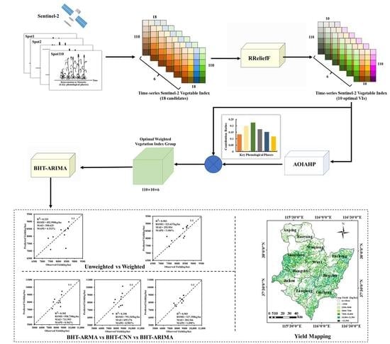
This study aims to use remote sensing (RS) time-series data to explore the intrinsic relationship between crop growth and yield formation at different fertility stages and construct a high-precision winter wheat yield estimation model applicable to short time-series RS data. Sentinel-2 images were acquired in this study at six key phenological stages (rejuvenation stage, rising stage, jointing stage, heading stage, filling stage, filling-maturity stage) of winter wheat growth, and various vegetation indexes (VIs) at different fertility stages were calculated. Based on the characteristics of yield data continuity, the RReliefF algorithm was introduced to filter the optimal vegetation index combinations suitable for the yield estimation of winter wheat for all fertility stages. The Absolutely Objective Improved Analytic Hierarchy Process (AOIAHP) was innovatively proposed to determine the proportional contribution of crop growth to yield formation in six different phenological stages. The selected VIs consisting of MTCI(RE2), EVI, REP, MTCI(RE1), RECI(RE1), NDVI(RE1), NDVI(RE3), NDVI(RE2), NDVI, and MSAVI were then fused with the weights of different fertility periods to obtain time-series weighted data. For the characteristics of short time length and a small number of sequences of RS time-series data in yield estimation, this study applied the multiplexed delayed embedding transformation (MDT) technique to realize the data augmentation of the original short time series. Tucker decomposition was performed on the block Hankel tensor (BHT) obtained after MDT enhancement, and the core tensor was extracted while preserving the intrinsic connection of the time-series data. Finally, the resulting multidimensional core tensor was trained with the Autoregressive Integrated Moving Average (ARIMA) model to obtain the BHT-ARIMA model for wheat yield estimation. Compared to the performance of the BHT-ARIMA model with unweighted time-series data as input, the weighted time-series input significantly improves yield estimation accuracy. The coefficients of determination (R²) were improved from 0.325 to 0.583. The root mean square error (RMSE) decreased from 492.990 to 323.637 kg/ha, the mean absolute error (MAE) dropped from 350.625 to 255.954, and the mean absolute percentage error (MAPE) decreased from 4.332% to 3.186%. Besides, BHT-ARMA and BHT-CNN models were also used to compare with BHT-ARIMA. The results indicated that the BHT-ARIMA model still had the best yield prediction accuracy. The proposed method of this study will provide fast and accurate guidance for crop yield estimation and will be of great value for the processing and application of time-series RS data.

1. Introduction

As one of the most widely planted crops globally, wheat yield prediction in large areas is essential to ensure food security and maintain sustainable agricultural development [1,2]. Traditional yield estimation methods mainly include statistical field surveys or sampling inspections, which are time-consuming and require a lot of manpower and material resources [3,4]. As a non-destructive emerging technology, remote sensing (RS) technology has the characteristics of high timeliness, wide coverage, and low cost [2], and is widely used in crop growth monitoring and yield prediction [5].

In recent decades, the use of assimilation methods to couple crop growth models with RS data has become one of the development trends in yield estimation. The crop growth model integrated multidisciplinary research (including crop physiology, ecology, meteorology, soil science, agronomy, etc.) to quantitatively and dynamically predict crop yield [6,7,8,9,10,11,12,13,14]. However, incomplete acquired localization data in practical applications will lead to serious bias and instability in crop field forecasting. Besides, the complexity of the agricultural system determines the uncertainty of assimilation, and a large number of data calculations also limit the accuracy of large-area yield estimation [15].

To simplify the calculation and improve the application of RS in regional yield estimation, some researchers have tried methods using the characteristic multispectral information and its derivatives, including characteristic vegetation indices (VI) based on one specific phenological period to construct a yield prediction model. However, the limited amount of information for a given growth period makes it difficult to track the entire process of yield formation during crop growth, and thus lacks accuracy and robustness [16,17,18,19,20,21,22,23,24,25,26].

The time-series data were arranged in the order of the size of the time stamp, which contains the dynamic information during a certain period. In recent years, the application of time-series data in agriculture has been more extensive, including crop mapping, yield estimation, etc. [27,28]. In crop yield estimation, the time-series RS data contain dynamic information on the growth and development of the crop throughout the growing season [29,30,31]. Using time-series data to estimate yields has become one of the research hot spots. Among the existing time-series forecasting (TSF) methods, Long Short-Term Memory (LSTM) [32], as a sort of deep learning method, has been widely used for crop yield estimation and prediction by its sequence modeling using a long-time memory function [33]. However, there is a large error in the parallel processing of multiple temporal data. In addition, Convolutional Neural Networks (CNN) [34] have also been increasingly used in yield estimation due to the shared convolutional kernels, which can achieve automatic feature extraction at the convolutional layer and greatly improve the efficiency of yield prediction. However, a large amount of information will be lost in the pooling layer [35]. Besides, the performance of the TSF models related to deep learning suffers badly when the amount of data is not enough, limiting these models’ use for yield estimation based on time-series RS data. Focusing on the shortages of the existing TSF models mentioned above, the Autoregressive Integrated Moving Average (ARIMA) [36] method could be used in yield estimation due to its simplicity and good statistical properties. In addition, in order to consider the intrinsic correlation between time-series data and further capture the interactions between nutrient and structural parameters with yield formation during crop growing, multiple delayed embedding transform (MDT) [37], an emerging technique, is used to perform tensor decomposition to obtain higher-order block Hankel tensor (BHT) [38]. The hybrid method combining the ARIMA and BHT can reduce information loss during tenderization, capture the intrinsic correlation of time series, solve insufficient experimental data to a certain extent, and has great potential in predicting winter wheat yield [39].

This study aims to propose a high-precision winter wheat yield estimation method applicable to short time-series RS data. Firstly, the optimal vegetation indices group suitable for yield estimation during six key growth periods of winter wheat was obtained based on the Regressional ReliefF (RReliefF) algorithm. Then, the Absolutely Objective Improved Analytic Hierarchy Process (AOIAHP) algorithm was innovatively proposed to determine the contribution weights of the different growth stages to winter wheat yield accumulation. For short time-series RS data prediction, the BHT-ARIMA was firstly applied in yield estimation to solve the problem of insufficient sampled data. The paper is organized as follows. Section 2 introduces the experiment design/data used in this study and describes the details regarding the proposed Absolutely Objective Improved Analytic Hierarchy Process and BHT-ARIMA model, etc. Results of selected optimal VIs, contribution ratio determination, and the winter wheat yield estimation are all described in Section 3. The comparison of the BHT-ARIMA model with other methods in yield estimation is discussed in Section 4. The paper concludes in Section 5 with a summary of the results.

2. Materials and Methods

2.1. Study Region

Hengshui City ($115°10’–116°34’\mathrm{E},37°03’–38°23’\mathrm{N}$), Hebei Province, China, was chosen as the study region. The region is part of the North China Plain, an alluvial plain of the Yellow River, Huaihe River, and Haihe River [40]. It is an important food production area in North China. In this region, winter wheat is the primary crop, and the main crop planting pattern is the rotation of winter wheat and summer maize [41]. Winter wheat was selected as a research crop in yield estimation.

2.2. Experiment Design

Field data measurement was conducted on the winter wheat only during the harvest time. Twenty-two fields, each of which has an area larger than 1 km², were selected and examined. Five plots were deployed diagonally in each field with distance of 50 m to each other and 50 m from the edge of a field, as shown in Figure 1. Then, 110 plots were selected for the experiment. Besides, the coordinates of the experimental plots were recorded by a Global Positioning System (GPS, Trimble GeoExplorer 6000 Series GeoXH, Trimble Navigation, Ltd., Sunnyvale, CA, USA) to accurately obtain corresponding band information from RS images.

2.3. Winter Wheat Yield Data

The growth of the farmland within the pixel scale of the Sentinel-2 was roughly uniform, so the yield per unit area (1 m²) was chosen as a representative of the point, and the distribution of winter wheat within one plot is shown in Figure 1. From each 1 m² plot, all ears of winter wheat were collected. According to the standard method of obtaining the dry weight of the winter wheat ears, the ears were heated to 105 °C for killing to inactivate enzymes to reduce the effect on dry weight and dried at 80 °C until a constant weight was reached in the laboratory. Next, the dried grains were manually collected from the ears, and the final dry weight of the grains was recorded with the unit of g. In addition, the unit was then converted from g/m² to kg/ha.

2.4. Sentinel-2 Image Processing

The whole growth period of winter wheat occurs from early March to late May. The selected periods of this study are from rejuvenation to filling-maturity. Predominantly cloud-free Sentinel-2 images covering the whole territory during the key phenological phases (Level 1C Top-of-Atmosphere reflectance products) were downloaded from the Copernicus Open-Access Hub (https://scihub.copernicus.eu/dhus/#/home, accessed on 1 July 2020), as shown in

Table 1. Sentinel-2 images covering dates and the phenology of winter wheat.

Time	March			April			May
	E-Mar	M-Mar	L-Mar	E-Apr	M-Apr	L-Apr	E-May	M-May	L-May
Phenological Phases	Rejuvenation	Rising		Jointing		Heading		Filling	Filling-Maturity
Dates of Sentinel-2 images (Day/Month/Year)	9 March 2017	29 March 2017		18 April 2017		28 April 2017		18 May 2017	28 May 2017

. Only one Sentinel-2 image was used for each phenological phase. Details of the bands used in this study can be found in

Table 2. Central wavelength and spatial resolution for the Sentinel-2 bands used in this study.

Spectral Band	Wavelength (nm)	Spatial Resolution (m)
Band 2 BLUE	496.6	10
Band 3 GREEN	560	10
Band 4 RED	664.5	10
Band 5 RED EDGE1	703.9	20
Band 6 RED EDGE2	740.2	20
Band 7 RED EDGE3	782.5	20
Band 8 NIR	835.1	10

. All bands were atmospherically corrected using the Sen2Cor processor tool, and the bands at 20 m resolution were rescaled to 10 m before being stacked [18,42].

2.5. Data Analysis

2.5.1. RReliefF

In order to quickly and effectively select the optimal VIs suitable for winter wheat yield estimation and their importance ranking from the VI candidates, the RReliefF algorithm [43], as an extended variant of Relief [44], was adopted to screen the optimal VIs with high efficiency. Unlike Relief, which is a typical binary classification algorithm, the RReliefF could cope with the feature selection with continuous target variables. The calculation workflow is shown below.

RReliefF first sets ranking factors R_dy, R_dj, R_dy∧dj, and R_j equal to 0. Then, the algorithm iteratively selects a random observation x_r, finds the k-nearest observations to x_r, and updates all the intermediate ranking factors, as follows [45]:

$$R_{dy}{}^i{=R}_{dy}{}^{i-1}+{\Delta }_y{(x}_R{,x}_q)·d_{rq}$$

(1)

$$R_{dj}{}^i{=R}_{dj}{}^{i-1}+{\Delta }_j{(x}_R{,x}_q)·d_{rq}$$

(2)

$$R_{dy\wedge dj}{}^i{=R}_{dy\wedge dj}{}^{i-1}+{\Delta }_y{(x}_R{,x}_q)·{\Delta }_j{(x}_R{,x}_q)\cdot d_{rq}$$

(3)

where R_dy is the ranking factor of having different values for the response y (i.e., the actual yields), R_dj is the ranking factor of having different values for the predictor F_j, and R_dy∧dj is the ranking factor of having different response values and different values for the predictor F_j. The i and i−1 superscripts denote the iteration step number. Δy(x_r,x_q) is the difference in the value of the continuous response y between observations x_r and x_q, shown as Equation (4). Let y_r denote the value of the response for observation x_r, and let y_q denote the value of the response for observation x_q. Δj(x_r,x_q) is the difference in the value of the predictor F_j between observations x_r and x_q, shown as Equation (5). Let x_rj denote the value of the jth predictor for observation x_r, and let x_qj denote the value of the jth predictor for observation x_q.

$${\Delta }_y\left(x_r,x_q\right)=\frac{\left|y_r-y_q\right|}{max\left(y\right)-min\left(y\right)}$$

(4)

$${\Delta }_j\left(x_r,x_q\right)=\frac{\left|x_{rj}-x_{qj}\right|}{max\left(F_j\right)-min\left(F_j\right)}$$

(5)

d_rq is a distance function of the form, shown as Equation (6), and the distance is subject to the scaling, $\widetilde{d_{rq}}$, shown as Equation (7):

$$d_{rq}=\frac{\widetilde{d_{rq}}}{{{\displaystyle \sum }}_{i=1}^k\widetilde{d_{rl}}}$$

(6)

$$\widetilde{d_{rq}}{=e}^{-{\left(rank\right(r,q\left)\right)}^2}$$

(7)

where rank(r,q) is the position of the qth observation among the nearest neighbors of the rth observation, sorted by distance, and k is the number of nearest neighbors.

Finally, the RReliefF calculates the predictor ranking factor R_j after fully updating all the intermediate ranking factors. m is the number of iterations.

$$R_j=\frac{R_{dy\wedge dj}}{R_{dy}}-\frac{R_{dj}-R_{dy\wedge dj}}{{m-R}_{dy}}$$

(8)

In this study, the RReliefF algorithm evaluated candidate VIs’ importance to the measured yields from the 110 sampling plots. Subsequently, the importance ranking of VIs can be obtained, which were taken as a standard of selecting optimal vegetation index combinations, as shown in Figure 2. A higher ranking of the VI obtained by RReliefF means that the VI has a closer relation with the yield formation, which laid a foundation for the contribution weights estimation and yield prediction to be discussed in Section 2.5.3. In this study, the top 10 features were selected for the following weight estimation and yield prediction.

2.5.2. Improved Analytic Hierarchy Process

Different phenological stages of winter wheat have different effects on the accumulation of winter wheat yield. It is crucial to determine the weights of each phenological stage scientifically and effectively using the results derived from the mathematical analysis of limited data.

The improved analytic hierarchy process (IAHP) is a weighting method that is optimized from the analytic hierarchy process (AHP) for solving fuzzy problems with incomplete information. A comparison matrix needs to be constructed at the beginning [3]. Compared with AHP, IAHP does not need a consistency test, avoiding adjusting the comparison matrix multiple times and improving efficiency and accuracy [3,46,47]. More importantly, IAHP uses the “three-scale method” to construct the comparison matrix, which means the elements in the matrix are just integers from 0 to 2, and these integers imply the degree of importance between the elements [47]. The values of the elements are determined by the subjective analysis of experts. In this study, IAHP only needed the ranking of the importance of the phenological periods to construct the comparison matrix, significantly reducing the amount of information needed to determine the weights and leveraging the results of mathematical data analysis.

2.5.3. Absolutely Objective Improved Analytic Hierarchy Process

IAHP makes it easier for experts to judge the importance of the comparison to construct the comparison matrix. However, it still requires experts to compare the importance of two stages affected by subjective factors to a certain extent [3,46,47]. The Absolutely Objective Improved Analytic Hierarchy Process (AOIAHP) is innovatively proposed in this paper to completely eliminate the influence of subjective factors. In AOIAHP, the objective data analysis determined the comparison matrix be constructed in the first step of IAHP. In this case, the AOIAHP improved the accuracy of weight calculation.

As shown in Figure 3, the selected ten VI time-series data points of six key phenological phases were used as the predictor variable vector to form the input matrices (110 × 6), and the yield data measured by different plots were used as a response vector (110 × 1). The importance ranking of six key phenological phases of winter wheat based on a single VI can be obtained after RReliefF analysis. Subsequently, the rankings were averaged among the selected ten VIs to obtain a total ranking vector of the six key phenological phases.

Based on the composite ranking of six key phenological phases, the comparison matrix, $\mathrm{A}\left(a_{ij}\right)$, shown as Equation (9), can be scientifically and objectively constructed:

$$\mathrm{A}\left(a_{ij}\right)=\left(\begin{array}{ccc}{a}_{11}& \cdots & a_{16}\\ ⋮& \ddots & ⋮\\ a_{61}& \cdots & a_{66}\end{array}\right)$$

(9)

The value of $a_{ij}$ is the comparison result related to the ranking of the importance of six key phenological stages of winter wheat. The values of i and j are both from 1 to 6, corresponding to the six key phenological wheat periods, as shown in Table 1, and the integer values of $a_{ij}$ are from 0 to 2, corresponding to period i being less important than period j, period i being equally important as period j, and period i being more important than period j, respectively.

Then, the importance coefficients vector, r, of winter wheat growth stages can be calculated using the elements in the comparison matrix, $\mathrm{A}\left(a_{ij}\right)$, shown as Equation (10):

$$r_j={\displaystyle \sum }_{i=1}^6{a}_{ij},j=1,2,\cdots ,6$$

(10)

where the subscript j for r indicates six key phenological periods of the winter wheat.

The judgment matrix, $\mathrm{B}\left(b_{ij}\right)$, can be constructed based on the importance coefficients of winter wheat key phenological stages, obtained by Equation (11):

$$\mathrm{B}\left(b_{ij}\right)=\left(\begin{array}{ccc}{b}_{11}& \cdots & b_{16}\\ ⋮& \ddots & ⋮\\ b_{61}& \cdots & b_{66}\end{array}\right)$$

(11)

$$b_{ij}=\{\begin{array}{c}\frac{r_i-r_j}{r_{max}-r_{min}}\times \left(\frac{r_{max}}{r_{min}}-1\right){+1,r}_i\ge r_j\\ {(\frac{r_j{-r}_i}{r_{max}{-r}_{min}}\times \left(\frac{r_{max}}{r_{min}}-1\right)+1)}^{-1},r_i<r_j\end{array},i=1,2,\cdots ,6;j=1,2,\cdots ,6$$

(12)

where r takes on different values depending on the subscript, and r_max and r_min are the maximum and minimum value of importance coefficients obtained by Equation (10), respectively.

Finally, the quasi-optimal matrix, $\mathrm{Q}\left(q_{ij}\right)$, can be obtained based on elements in $\mathrm{B}\left(b_{ij}\right)$, shown as Equation (13), obtained by Equation (14):

$$\mathrm{Q}\left(q_{ij}\right)=\left(\begin{array}{ccc}{q}_{11}& \cdots & q_{16}\\ ⋮& \ddots & ⋮\\ q_{61}& \cdots & q_{66}\end{array}\right)$$

(13)

$$q_{ij}{=10}^{\frac{1}{6}{\displaystyle \sum }_{T=1}^{6}lg(\frac{b_{it}}{b_{jt}})},i=1,2,\cdots 6;j=1,2,\cdots ,6$$

(14)

where the value of $q_{ij}$ can be calculated by Equation (14) using the elements of the matrix $\mathrm{B}\left(b_{ij}\right)$.

The weight vector, $\mathit{W}$, of six key phenological phases can be obtained based on the maximum eigenvalue and the maximum eigenvector, d, of the quasi-optimal matrix $\mathrm{Q}\left(q_{ij}\right)$. The elements of W can be obtained by Equation (15), where ${\displaystyle \sum }_{k=1}^6{{\displaystyle w}}_k=1$, and k refers to 6 key phenological phases:

$$w_k=\frac{d_k}{{{\displaystyle \sum }}_{i=1}^6{d}_i},k=1,2,\cdots ,6$$

(15)

Finally, with the obtained weights of the six phenological phases, the optimal weighted vegetation index matrix (110 × 10 × 6) can be constructed, as shown in Figure 3.

2.6. BHT-ARIMA Model

The BHT-ARIMA model could fully exploit the intrinsic linkage of the time series and achieve augmentation of short time-series data, effectively solving the problem of simultaneous prediction of multiple short time-series data points [48]. The specific steps of modeling are as follows [48]:

(1)

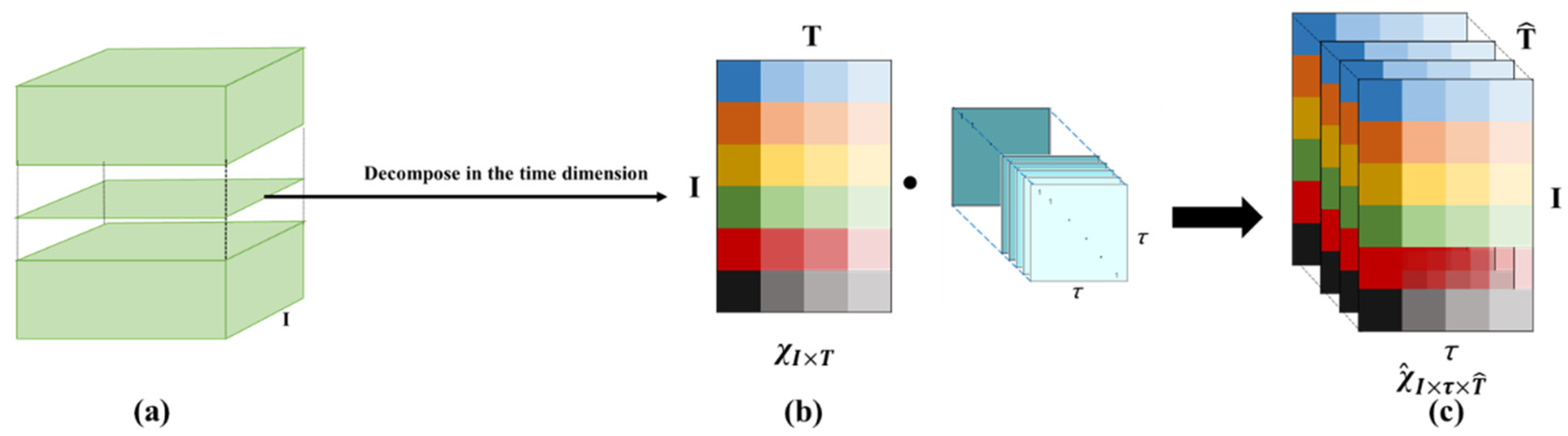
Obtain the high-order multidimensional short time-series data using MDT. As is shown in Figure 4, the ten calculated optimal weighted vegetation index time-series data points of six key phenological phases from different experimental plots, whose total number is I (110 herein), are decomposed in time dimension with the time decomposition number parameter, T, to obtain the decomposed time-series data, ${\left\{\chi \right\}}_{I\times T}$. High-order time-series data, ${\left\{{\widehat{\chi }}_t\right\}}_{I\times \tau \times \widehat{T}}=\left\{{\widehat{\chi }}_1,{\widehat{\chi }}_2,\cdots ,{\widehat{\chi }}_{\widehat{T}}\right\}$ , are obtained by stretching the decomposed time-series data, ${\left\{\mathsf{\chi }\right\}}_{I\times T}$, with the replication matrix, which is determined by the parameter $\tau$. The relationship between $T$ and $\widehat{T}$ is shown in Equation (16):

$$\widehat{T}=T-\tau +1$$

(16)

(2)

Obtain core tensors from the BHT by Tucker decomposition [49]. With the BHT, we compute its d-order differences to obtain a M-order tensor, $\left\{{\mathsf{\Delta }}^d{\widehat{\chi }}_t\right\}=\left\{{\mathsf{\Delta }}^d{\widehat{\chi }}_1,{\mathsf{\Delta }}^d{\widehat{\chi }}_2,\cdots ,{\mathsf{\Delta }}^d{\widehat{\chi }}_{\widehat{T}}\right\}$ [50]. After Tucker decomposition, $\left\{{\mathsf{\Delta }}^d{\widehat{\chi }}_t\right\}$ is decomposed into the product of a core tensor, $\left\{{\mathsf{\Delta }}^d{\widehat{G}}_t\right\}=\left\{{\mathsf{\Delta }}^d{\widehat{G}}_1,{\mathsf{\Delta }}^d{\widehat{G}}_2,\cdots ,{\mathsf{\Delta }}^d{\widehat{G}}_{\widehat{T}}\right\}$, and M orthogonal projection matrices, $\left\{{\widehat{U}}^{(m)}\right\}=\left\{{\widehat{U}}^{(1)},{\widehat{U}}^{(2)},\cdots ,{\widehat{U}}^{(M)}\right\}$, which are shown as below:

$${\mathsf{\Delta }}^d{\widehat{G}}_t={\mathsf{\Delta }}^d{\widehat{\chi }}_t\times {}_1\widehat{U}^{{(1)}^T}\cdots \times {}_m\widehat{U}^{{(m)}^T}$$

(17)

$$s. t. {\widehat{U}}^{{(m)}^T}{\widehat{U}}^{(m)}=I$$

(18)

where $m=1,2,\cdots ,M$, and $\left\{{\widehat{U}}^{(m)}\right\}$ are the projection matrices, which could maximally preserve the temporal continuity between core tensors, and $\left\{{\mathsf{\Delta }}^d{\widehat{G}}_t\right\}$ are the low-rank core tensors, which could represent the important original information of Hankel and the intrinsic linkage of the time-series data.

(3)

Tensorized ARIMA model establishment. To retain the temporal correlations among core tensors, a (p; d; q)-order ARIMA model is constructed in the tensor form, which could be used to connect the current core tensor, $\left\{{\mathsf{\Delta }}^d{\widehat{G}}_t\right\}$ and the previous core tensors, $\left\{{\mathsf{\Delta }}^d{\widehat{G}}_{t-1},{\mathsf{\Delta }}^d{\widehat{G}}_{t-2},\cdots ,{\mathsf{\Delta }}^d{\widehat{G}}_{t-p}\right\}$, as in Equation (19). $\left\{{\alpha }_i\right\}$ and $\left\{{\beta }_i\right\}$ are the coefficients of the autoregressive model (AR) and the moving average model (MA), respectively, which were estimated from the core tensors and the residual time-series data [39,51]. $\left\{{\widehat{\epsilon }}_{t-i}\right\}$ are the random errors of past q observations, and $\left\{{\widehat{\epsilon }}_t\right\}$ is the forecast error at the current time point, which should be minimized to optimal zero.

$${\mathsf{\Delta }}^d{\widehat{G}}_t={\displaystyle \sum }_{i=1}^p{\alpha }_i{\mathsf{\Delta }}^d{\widehat{G}}_{t-i}-{\displaystyle \sum }_{i=1}^q{\beta }_i{\widehat{\epsilon }}_{t-i}+{\widehat{\epsilon }}_t$$

(19)

where $\left\{{\mathsf{\Delta }}^d{\widehat{G}}_t\right\}$ is input into the tensorized ARIMA model to forecast a new core tensor, $\left\{{\mathsf{\Delta }}^d{\widehat{G}}_{t+1}\right\}$. Back projection used $\left\{{\widehat{U}}^{(m)}\right\}$ to obtain $\left\{{\mathsf{\Delta }}^d{\widehat{\chi }}_{\widehat{T}+1}\right\}$ to get the predicted values at the $\widehat{T}+1$ time point for all the time-series data simultaneously, which is shown in Equation (20). Finally, inverse differencing and inverse-MDT were applied to obtain the prediction result $\left\{{\chi }_{T+1}\right\}$.

$${\mathsf{\Delta }}^d{\widehat{\chi }}_{\widehat{T}+1}={\mathsf{\Delta }}^d{\widehat{G}}_{t+1}\times {}_1\widehat{U}^{{(1)}^T}\cdots \times {}_m\widehat{U}^{{(m)}^T}$$

(20)

In this study, the BHT-ARIMA model was applied to estimate the yield of the winter wheat based on short RS time-series data. Five key model parameters required special attention when predicting winter wheat yields using the BHT-ARIMA model, as shown in

Table 3. Setting of BHT-ARIMA parameters.

Parameter	Value	Note
Number of time-series data points of single VI (I)	110	Determined by the original dataset
Number of selected optimal VIs	10	Determined by the original dataset
Time decomposition number parameter (T)	10	Determined manually, integer multiples of 10
Replication matrix parameter ($\tau$)	5	Determined manually, integers less than T
Number of TS layers ($\widehat{T}$)	6	Calculated by Equation (16)

. The number of time-series data points of single VI (I) and the number of selected optimal VIs were determined by the original dataset. The number of time-series data points of single VI (I) is the amount of time-series data for each single VI. There were 110 sets of time-series data representing 110 experimental plots for each single VI. The meaning of the number of selected optimal VIs is obvious. It represents the number of VIs selected to be input into the BHT-ARIMA. The number of selected optimal VIs was set to 10, as 10 VIs had the best prediction performance and reduced the complexity of the model calculation, which was proven in Section 3.3.2. The time decomposition number parameter (T) and the replication matrix parameter (τ) were determined manually according to the model characteristics. The time decomposition number parameter (T) was related to time-series segmentation, an integer that is limited to an integer multiple of 10. The replication matrix parameter (τ) was an integer less than the time decomposition number parameter (T). The number of TS layers ($\widehat{T}$) was calculated from the time decomposition number parameter (T) and the replication matrix parameter (τ), as shown in Equation (16). The specific parameter values and notes are summarized in Table 3.

Although the BHT-ARIMA model utilized complex data processing techniques such as tensor decomposition, this algorithm did not need to copy data or pack existing data, but wrote data directly to the tensor, and no additional copies were created for both in-process and out-of-process execution. Therefore, this algorithm did not require high hardware configuration. The algorithm’s arithmetic power requirement was 30 g of semi-precision, which can be run 783 times per second according to the theoretical value, and the peak bandwidth was about 540 GB/s under the common RTX 2070 graphics card environment, so it only took a few minutes to obtain the prediction results of this model.

2.7. Prediction Accuracy Evaluation

In this study, the coefficient of determination (R-square, $R^2$), mean absolute error (MAE), mean absolute percentage error (MAPE), and root mean square error (RMSE) were used to determine the predictive performance of the model. The $R^2$, MAE, MAPE, and RMSE were defined as follows:

$$R^2=1-\frac{{{\displaystyle \sum }}_{i=1}^n \left(y_i^{\text{'}}-\bar{y}\right)}{{{\displaystyle \sum }}_{i=1}^n \left(y_i-\bar{y}\right)}$$

(21)

$$\mathrm{MAE}=\frac{1}{n}{\displaystyle \sum }_{i=1}^n{|y}_i{-y}_i^{’}|$$

(22)

$$\mathrm{MAPE}=\frac{1}{n}{\displaystyle \sum }_{i=1}^n|\frac{y_i-y_i^{’}}{y_i}|\times 100\%$$

(23)

$$\mathrm{RMSE}=\sqrt{\frac{1}{n}{\displaystyle \sum }_{i=1}^n{{(y}_i-y_i^{’})}^2}$$

(24)

where n represents the number of samples, $y_i$ is the observed yield value, $y_i^{’}$ is the predicted yield, and $\overline{y}$ is the average observed yield.

3. Results and Analysis

3.1. Growth Analysis of Winter Wheat Based on Optimal VIs during the Whole Growth Period

3.1.1. Initial Vegetation Index Candidates

VIs shown in Table 3 were initially chosen as candidates for the following selection. All these VIs have been proven to have a close correlation with crop nutritional parameters (such as chlorophyll, nitrogen, etc.) and structural parameters (leaf area index (LAI), etc.). VIs, including NDVI [17,18,20], GNDVI [21], MTCI [22], WDRVI [24,25], etc., have often been used directly to build linear regression models for yield estimation. In addition, some characteristic VIs, including REP [23] and SAVI [52], etc., have proven to be highly correlated with crop nutrition parameters. Besides, VIs including NDVI [53,54], WDRVI [55,56], etc., have been applied to measure structural parameters (LAI, etc.). These indexes can also be used to reflect crop yield from the aspect of nutrition. Three red-edge bands in Sentinel-2 were used in the study, so VIs including NDRE, MTCI, and CI_RE with red-edge bands (abbreviated as RE) were calculated using different red-edge bands, including RE1, RE2, and RE3, in order to take full advantage of multiple red-edge bands in Sentinel-2. A total of 18 VIs were obtained for the following selection. The specific calculation equations using the bands shown in Table 2 are shown in the middle column in

Table 4. Initial vegetation index candidates.

Vegetation Index	Description	References
Normalized Difference Vegetation Index (NDVI)	$(\mathrm{NIR}-\mathrm{RED})/(\mathrm{NIR}+\mathrm{RED})$	[57]
Normalized Difference Red-Edge Index (NDRE)	$(\mathrm{NIR}-\mathrm{RE})/(\mathrm{NIR}+\mathrm{RE})$	[58]
Green Normalized Difference Vegetation Index (GNDVI)	$(\mathrm{NIR}-\mathrm{GREEN})/(\mathrm{NIR}+\mathrm{GREEN})$	[59]
Wide Dynamic Range Vegetation Index (WDRVI)	$(0.2\times \mathrm{NIR}-\mathrm{RED})/(0.2\times \mathrm{NIR}+\mathrm{RED})$	[60]
Enhanced Vegetation Index (EVI)	$2.5\times (\mathrm{NIR}-\mathrm{RED})/(\mathrm{NIR}+6\times \mathrm{RED}+7\times \mathrm{BLUE}-1)$	[61]
Two-band Enhanced Vegetation Index (EVI2)	$(\mathrm{NIR}-\mathrm{RED})/(\mathrm{NIR}+2.4\times \mathrm{RED}+1)$	[62]
MERIS Terrestrial Chlorophyll Index (MTCI)	$(\mathrm{NIR}-\mathrm{RE})/(\mathrm{NIR}-\mathrm{RED})$	[63]
Green Chlorophyll Vegetation Index (GCVI)	$(\mathrm{NIR}/\mathrm{GREEN})-1$	[64]
Chlorophyll Index Red-Edge (CIRE)	$(\mathrm{NIR}/\mathrm{RE})-1$	[64]
Modified Soil-Adjusted Vegetation Index (MSAVI)	$\frac{1}{2}(2\times \mathrm{NIR}+1-\sqrt{{(2\times \mathrm{NIR}+1)}^2-8\times (\mathrm{NIR}-\mathrm{RED})})$	[65]
Optimization Soil-Adjusted Vegetation Index (OSAVI)	$1.16\times (\mathrm{NIR}-\mathrm{RED})/(\mathrm{NIR}+\mathrm{RED}+0.16)$	[66]
Red-Edge Position Index (REP)	$700+40\times \left(\right(\mathrm{RED}+\mathrm{RE}3)/2-\mathrm{RE}1)/(\mathrm{RE}2-\mathrm{RE}1)$	[67]

.

3.1.2. Optimal VI Selection to Monitor the Growth of Winter Wheat

Among the VI candidates, the optimal VIs for yield estimation during the whole growth period were selected through the RReliefF algorithm and shown in

Table 5. Optimal VIs for field estimation during the whole growth period.

Rank	Vegetation Index
1	MTCI(RE2)
2	EVI
3	REP
4	MTCI(RE1)
5	RECI(RE1)
6	NDVI(RE1)
7	NDVI(RE3)
8	NDVI(RE2)
9	NDVI
10	MSAVI

, which are sensitive to the chemical and biophysical parameters, which determined the photosynthetic capacity and efficiency and further affected yield formation of winter wheat [68]. As is shown in this table, the red-edge band of Sentinel-2 was fully utilized. According to the published literature, MTCI was closely related to the chlorophyll content of crops, which is the basic element for photosynthesis [63,69]. Besides, MTCI is highly sensitive to changes in biomass during the whole growth period of winter wheat [70]. REP strongly correlates with a wide range of foliar N concentrations during the whole growth period, influencing photosynthesis and yield formation [23,71]. These are consistent with the stable and high ranking of MTCI and REP by RReliefF. NDVI is one of the most widely used VIs to evaluate crop growth and monitor the nutrients needed for crop growth, development, and yield estimation. Besides, NDVI(RE), calculated from the red-edge bands, red edge1, red edge2, and red edge3, delays the saturation trend during the late growth period [70]. Additionally, EVI was proposed to handle the saturation problem of NDVI with improved sensitivity in high-biomass regions and improved vegetation monitoring through a de-coupling of the canopy background signal and a reduction in atmosphere influences [68,72]. SAVI and its optimized variants (MSAVI, OSAVI) increased vegetation reflection while suppressing soil background effects in images to improve monitoring accuracy [65,66]. The above reviews verified that the combination of selected VIs could give full play to their respective advantages in crop growth monitoring and yield forecasting during the whole growth period of winter wheat.

3.2. Contribution Ratio Determination to Winter Wheat Yield Accumulation

Based on AOIAHP, the contribution ratios of six key growth stages can be obtained. Figure 5 presents the bar chart of the contribution ratios of six key phenological phases, showing that the jointing period had the highest contribution ratio, followed by the rising, heading, filling, rejuvenation, and lastly, filling-maturity period.

In the rejuvenation period, yellow leaves of winter wheat turned green as the canopy structure and chemical parameter content of winter wheat increased. From the rising period to jointing, chemical and biophysical parameters influencing photosynthesis continued to increase, increasing contribution ratios to yield. From the jointing period to the heading period, the growth and development of winter wheat dramatically increased, with the root group and the leaf area reaching the maximum, and the wheat ears beginning to differentiate. These stages are the key periods for determining the number of grains per ear, and it is also the consolidation period for the effective number of ears per hectare and the weight. After the heading period, starch, protein, and accumulated organic matter produced by photosynthesis are stored in the grain through assimilation, still determining the accumulation of winter wheat.

3.3. Winter Wheat Yield Prediction and Analysis

3.3.1. Winter Wheat Yield Prediction Based on Optimal Weighted Vegetation Indexes and the BHT-ARIMA Model

This research used six phenological phases weighted VI time series to establish the BHT-ARIMA model to predict winter wheat yield. The 110 samples were divided into 2 parts for model establishment, where 88 samples were selected randomly for use as the calibration subset, and the remaining 22 were used as the independent validation subset. The R², RSME, MAE, and MAPE for the relationship between the observed and predicted yields in the validation dataset were calculated to evaluate the performance of the prediction of the BHT-ARIMA model. The input of the tensorized ARIMA model (i.e., BHT-ARIMA) has to meet the data requirements of the ARIMA model. The final BHT-ARIMA model only outputs ten reasonable data points after eliminating the unreasonable data. As shown in Figure 6, the R-square reached 0.583 and the RSME, MAE, and MAPE of this model were 323.637 kg/ha, 255.954, and 3.186%, respectively. This model performed better when the observed yields were larger than 8000 kg/ha. The good performance shows that the BHT-ARIMA model has capability in short time-series forecasting in agriculture.

The vegetation index information was constant for each sample when the model was trained. To demonstrate whether the model was overfitted on the VIs, we trained the model with randomly selected yield samples from 80% of all samples, using other samples for cross-validation. The cross-validation is to verify whether the model is overfitted. With the increase in the number of verifications, overfitting can likely occur if the difference between training and validation errors is significant. In this case, the R² was used as the only metric to measure the cross-validation results. This validation was performed ten times. As we can see from Figure 7, R² fluctuated around 0.5. The result indicated no significant overfitting, which implies that the model is generalized and can be used to estimate winter wheat yield. However, only ten reasonable results were obtained after data tensorization, the sample pool was reduced, which also had some influence on the validation process, and there were some limitations of this method.

3.3.2. Influence of the Number of Vegetation Indexes on the Performance of the BHT-ARIMA Model

In order to analyze the effect of the number of vegetation indices we selected on the model prediction performance, 18 matrices ranging in size from 110 × 1 × 6 to 110 × 18 × 6 were used sequentially as inputs to the BHT-ARIMA model. The R², RSME, MAE, and MAPE were calculated to assess the performance of the BHT-ARIMA model, as shown in Figure 8. Figure 8a shows that R² basically had an increasing trend, with the increase of the number of the selected indexes less than 10, and stabilized when the number was larger than 10. Figure 8b–d show that the RSME, MAE, and MAPE had approximately the same trend. They declined with high fluctuations and had larger values before ten. When the number of the selected indexes was greater than ten, the values of all three parameters gradually leveled off.

However, if too many indexes were selected, for each additional set of indexes, the BHT-ARIMA model needed to perform the process of tensor transformation, decomposition, and inversion again, which made the calculation cycle longer, increased the burden of the system, and reduced the efficiency of the model and redundancy.

Therefore, ten VIs selected by the RReliefF algorithm were used as model inputs to obtain better prediction results while saving computational cycles and maximizing model efficiency. Besides, the results indicated that the ten selected sets of vegetation index can represent valid information related to yield formation and effectively reduce the redundancy of information from the full vegetation index.

3.3.3. Comparisons of Performance of Weighted Vegetation Indexes and Unweighted Vegetation Indexes in the BHT-ARIMA Model

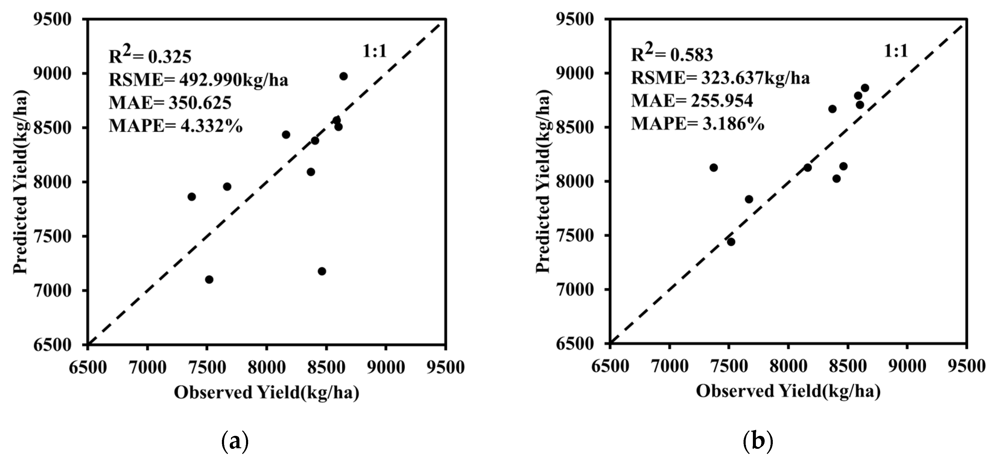
In order to verify the effect of the calculated weights on different phenological periods for winter wheat yield accumulation, two datasets of winter wheat VIs were established, including the dataset used in Section 3.3.1, i.e., the weighted optimal vegetation index group, and the dataset of the unweighted optimal vegetation index group. The samples were divided into two groups: 80% were the calibration group and the remaining 20% were the validation group. Figure 8 shows the scattered plots of the predicted yield and real winter wheat yield, which were predicted based on the unweighted and weighted optimal VI groups. Since the tensorized ARIMA model specifies non-zero input values, the model has only 10 sets of output values after automatically eliminating the unreasonable values. Figure 9 shows that the predicted yield was positively correlated with the observed yield. Figure 9a,b are the plots of the relationship between the predicted yield and the observed yield using unweighted and weighed VI groups, respectively. The R-square of the calibrated model with weighted VI reached 0.583, higher than that of the model with unweighted VI, whose R-square reached 0.325. The weighted model’s RSME, MAE, and MAPE were 323.637 kg/ha, 255.954, and 3.186%, respectively, smaller than those of the unweighted model, with 492.990 kg/ha, 350.625, and 4.332%, respectively.

The results indicate different degrees of influence on winter wheat yield for each phenological stage of winter wheat. The selected vegetation index combined with the contribution of key phenological stages can predict the yield of winter wheat well, with good robustness and realism.

3.3.4. Comparisons of Performance of BHT-ARMA, BHT-CNN, and BHT-ARIMA Models in Winter Wheat Yield Estimation

To verify the advantages of the BHT-ARIMA model in predicting winter wheat yield using short time-series RS data, BHT-ARMA and BHT-CNN models were applied to compare the performance in winter wheat yield estimation among the BHT-ARMA, BHT-CNN, and BHT-ARIMA models. BHT-ARMA and BHT-CNN models are tensorized from the original autoregressive moving average (ARMA) and CNN models. The CNN network is divided into five convolutional layers, four pooling layers, and two fully connected layers. Optimal weighted VI time-series data consisting of 10 selected VIs were used to train the BHT-ARIMA, BHT-ARMA, and BHT-CNN models and further evaluate the yield estimation accuracies of the trained models. The R², RSME, MAE, and MAPE for the observed and predicted yields’ relationship were calculated. The yield prediction results using the three methods mentioned above are shown in Figure 10.

As we can see from Figure 9, the overall performance of the BHT-ARIMA model was better than that of the BHT-ARMA and BHT-CNN models. The R² of the BHT-ARIMA model reached 0.583, higher than that of the BHT-ARMA and BHT-CNN models, with 0.302 and 0.350, respectively. Moreover, the MAE, MAPE, and RMSE of the BHT-ARIMA model, which were 284.366, 3.498%, and 327.358 kg/ha, respectively, were all lower than the BHT-ARMA model, with 711.993, 8.562%, and 958.730 kg/ha, and the BHT-CNN model with 695.276, 8.503%, and 791.545 kg/ha, respectively. The experimental data, including R², RSME, MAE, and MAPE, are summarized in

Table 6. The R², RSME, MAE, and MAPE of predictions using the BHT-ARMA, BHT-CNN, and BHT-ARIMA models.

Model	R2	RMSE (kg/ha)	MAE	MAPE (%)
BHT-ARMA	0.302	958.730	711.993	8.562
BHT-CNN	0.350	791.545	695.276	8.503
BHT-ARIMA	0.583	327.358	284.366	3.498

.

The results of the model performance comparison showed that the BHT-ARIMA model outperformed traditional deep learning networks and time-series prediction models in solving prediction problems for short time series of agricultural remote sensing, especially for multiple short time-series data prediction problems. Especially, we can see intuitively from Table 6 that, compared with BHT-ARMA and BHT-CNN, the R² of BHT-ARIMA had a dramatic rise from around 0.3 to around 0.6, while RMSE, MAE, and MAPE had a sharp decline. This may be caused by insufficient time-series data used in this study. Traditional prediction models require large, extensive data, limiting their application to yield predictions with fewer data. The BHT-CNN model was trained with a large amount of information that may be lost in the pooling layer, and the training results tended to converge on local minima, ignoring the local-to-whole correlation. The BHT-ARMA may not perform autoregressive learning, and only used data from the 10 sets of VIs with larger weights to predict. These limitations mentioned above became obvious when the input data were insufficient. In contrast, the BHT-ARIMA model made full use of the intrinsic linkage of the time series, automatically enabling data expansion for short time series.

3.3.5. Regional Winter Wheat Yield Estimation in Hengshui

In Section 3.3.1, the BHT-ARIMA model effectively estimated winter wheat yield based on short time-series VIs and actual yields, with R² reaching 0.583 from 110 experimental plots. In this section, the trained BHT-ARIMA model was used to estimate the regional winter wheat yields in Hengshui City, Hebei Province, based on the image of the winter wheat plant area. The data of the plant area of winter wheat in Hengshui City are from the published literature [40]. The prediction results are shown in Figure 11. Most predicted winter wheat yields in Hengshui City were between 7500 and 10,000 kg/ha, which was in line with the actual yield data in Section 2.3. In the west, mid-south, and east of Hengshui City, the predicted yields were higher than those of other areas in Hengshui City. Especially, the middle and south of Shenzhou, the east of Fucheng, and the east and south of Jingxian County were the higher-yield regions. These results were in general agreement with the spatial variation trend of the field experiment. The above results prove that the BHT-ARIMA model has strong spatial generalization in winter wheat yield estimation.

4. Discussion

Previous studies have explored correlations between multitemporal VIs and crop yields based on Random Forest (RF), Support Vector Machines (SVM), etc. However, these traditional deep learning-based methods require large, extensive data, limiting their application to yield predictions with fewer data [73,74,75,76]. Therefore, the BHT-ARIMA model applied in yield estimation has greater potential than other methods. In this study, BHT was obtained and combined with the ARIMA model, which can reduce information loss during tensorization, capture the intrinsic correlation of time series, and solve the problem of insufficient experimental data. The BHT-ARIMA model outperformed the BHT-ARMA and BHT-CNN models in estimating wheat yields, as mentioned in Section 3.3.4. In

Table 7. Comparisons of different RS methods for winter wheat yield estimation.

Model	Scale of Time-Series Data	R2	RMSE (t/ha)	Reference
PLS	UAV	0.45	1.84	[77]
SVM	UAV	0.50	1.75	[77]
RF	UAV	0.55	1.66	[77]
SVM	Ground	0.62	0.35	[41]
ACPM	Satellite	0.49	0.59	[40]
BHT-ARIMA	Satellite	0.58	0.32	This study

, we have summarized several published RS methods for winter wheat yield estimation, which all used multi-temporal time-series data. At the satellite scale, the Agriculture Crop Photosynthesis Model (ACPM) was proposed in [40] for the winter wheat aboveground biomass (DAM) and yield estimation, with R² around 0.49. It is worth noting that the measured yield data used in [40] were the same as the yield data in this study. In [41], SVM was applied to predict winter wheat yield based on ground-measured time-series spectral data. Its R² was larger than that of BHT-ARIMA, which may be caused by the larger scale of satellite data. In [77], based on UAV-scale RS time-series data, the PLS, SVM, and RF methods achieved yield prediction with R² of 0.45, 0.50, and 0.55, respectively, which were all less than the R² value of BHT-ARIMA.

The results showed the potential and advantages of BHT-ARIMA in the estimation of yield based on multi-temporal RS time-series data. However, it should be noted that in the tensorization process, the inversion of the tensor generated some outliers that did not meet the data requirements of the ARIMA model. In this case, some unreasonable data were lost automatically before being input into the ARIMA model, which impacts prediction accuracy.

5. Conclusions

This study aimed to use RS time-series data, explore the intrinsic relationship between crop growth and yield formation at different fertility stages, and construct a high-precision winter wheat yield estimation model applicable to short time-series data.

The ten optimal VIs, consisting of MTCI(RE2), EVI, REP, MTCI(RE1), RECI(RE1), NDVI(RE1), NDVI(RE3), NDVI(RE2), NDVI, and MSAVI, which were suitable for yield estimation at six key phenological phases, were obtained by the RReliefF algorithm. These selected VIs were not only relevant to yield formation mechanisms, efficiently predicting winter wheat yield, but also effectively reduced redundancy and computational effort.

Furthermore, AOIAHP was proposed to quantify the different effects of winter wheat growth on yield accumulation at different fertility stages. The jointing period had the highest contribution ratio to winter wheat yield accumulation, followed by rising, heading, filling, rejuvenation, and lastly, filling-maturity. The contribution ratios of the six key phenological stages could be used as weights to be combined with the selected VIs to predict winter wheat yields

Moreover, the BHT-ARIMA model was first applied to predict winter wheat yield with short time-series data. Compared with the BHT-CNN and BHT-ARMA models, the BHT-ARIMA model achieved the best prediction results, with R² reaching 0.583. The MAE, MAPE, and RMSE of the BHT-ARIMA model were lower than those of the BHT-ARMA and BHT-CNN models.

In this study, the BHT-ARIMA model improved the accuracy of winter wheat yield prediction based on weighted short RS time-series data, and its spatial generalization was proven. To further validate the generalization of the BHT-ARIMA model, in future work, we will validate the model for yield estimation in different regions, at different times, and for different crops to explore the universality and robustness of the model. As for the BHT-ARIMA model itself, we will improve the prediction accuracy of BHT-ARIMA, reducing the impact of data reduction due to the automatic elimination of the unreasonable values. This study provides a fast and accurate guide for crop yield prediction and will be of great value for the processing and applying of short RS time-series data.

References

- Chen, Z.; Ren, J.; Tang, H.; Shi, Y.; Leng, P.; Liu, J.; Wang, L.; Wu, W.; Yao, Y. Progress and Perspectives on Agricultural Remote Sensing Research and Applications in China. J. Remote Sens. 2016, 20, 748–767. [Google Scholar]
- Weiss, M.; Jacob, F.; Duveiller, G. Remote Sensing for Agricultural Applications: A Meta-Review. Remote Sens. Environ. 2020, 236, 111402. [Google Scholar] [CrossRef]
- Luo, S.; He, Y.; Li, Q.; Jiao, W.; Zhu, Y.; Zhao, X. Nondestructive Estimation of Potato Yield Using Relative Variables Derived from Multi-Period LAI and Hyperspectral Data Based on Weighted Growth Stage. Plant Methods 2020, 16, 1–14. [Google Scholar] [CrossRef] [PubMed]
- Li, S.; Ding, X.; Kuang, Q.; Ata-UI-Karim, S.T.; Cheng, T.; Liu, X.; Tian, Y.; Zhu, Y.; Cao, W.; Cao, Q. Potential of UAV-Based Active Sensing for Monitoring Rice Leaf Nitrogen Status. Front. Plant Sci. 2018, 9, 1834. [Google Scholar] [CrossRef] [PubMed] [Green Version]
- Yang, B.; Pei, Z. Definition of Crop Condition and Crop Monitoring Using Remote Sensing. Trans. CSAE 1999, 15, 214–218. [Google Scholar]
- Sinclair, T.R.; Seligman, N.G. Crop Modeling: From Infancy to Maturity. Agron. J. 1996, 88, 698–704. [Google Scholar] [CrossRef]
- Cao, J.; Jing, Q.; Zhu, Y.; Liu, X.; Zhuang, S.; Chen, Q.; Cao, W. A Knowledge-Based Model for Nitrogen Management in Rice and Wheat. Plant Prod. Sci. 2009, 12, 100–108. [Google Scholar] [CrossRef]
- Wiegand, C.L.; Richardson, A.J.; Jackson, R.D.; Pinter, P.J.; Aase, J.K.; Smika, D.E.; Lautenschlager, L.F.; McMurtrey, J.E. Development of Agrometeorological Crop Model Inputs from Remotely Sensed Information. IEEE Trans. Geosci. Remote Sens. 1986, GE-24, 90–98. [Google Scholar] [CrossRef]
- Delecolle, R.; Kuchar, L. Linear Correction of Model-Based Crop Biomass Simulations Using Intermediate Field Observations. Zesz. Probl. Postępów Nauk Rol. 1992, 398, 19–25. [Google Scholar]
- Faivre, R.; Fischer, A. Predicting Crop Reflectances Using Satellite Data Observing Mixed Pixels. J. Agric. Biol. Environ. Stat. 1997, 2, 87–107. [Google Scholar] [CrossRef]
- Moulin, S.; Bondeau, A.; Delecolle, R. Combining Agricultural Crop Models and Satellite Observations: From Field to Regional Scales. Int. J. Remote Sens. 1998, 19, 1021–1036. [Google Scholar] [CrossRef]
- Yue, J.; Feng, H.; Li, Z.; Zhou, C.; Xu, K. Mapping Winter-Wheat Biomass and Grain Yield Based on a Crop Model and UAV Remote Sensing. Int. J. Remote Sens. 2021, 42, 1577–1601. [Google Scholar] [CrossRef]
- Jin, N.; Tao, B.; Ren, W.; He, L.; Zhang, D.; Wang, D.; Yu, Q. Assimilating Remote Sensing Data into a Crop Model Improves Winter Wheat Yield Estimation Based on Regional Irrigation Data. Agric. Water Manag. 2022, 266, 107583. [Google Scholar] [CrossRef]
- Yang, S.; Hu, L.; Wu, H.; Ren, H.; Qiao, H.; Li, P.; Fan, W. Integration of Crop Growth Model and Random Forest for Winter Wheat Yield Estimation from UAV Hyperspectral Imagery. IEEE J. Sel. Top. Appl. Earth Obs. Remote Sens. 2021, 14, 6253–6269. [Google Scholar] [CrossRef]
- Huang, J.; Gómez-Dans, J.L.; Huang, H.; Ma, H.; Wu, Q.; Lewis, P.E.; Liang, S.; Chen, Z.; Xue, J.-H.; Wu, Y. Assimilation of Remote Sensing into Crop Growth Models: Current Status and Perspectives. Agric. For. Meteorol. 2019, 276, 107609. [Google Scholar] [CrossRef]
- Ren, J.; Chen, Z.; Zhou, Q.; Liu, J.; Tang, H. MODIS Vegetation Index Data Used for Estimating Corn Yield in USA. J. Remote Sens. 2015, 19, 568–577. [Google Scholar] [CrossRef]
- Labus, M.P.; Nielsen, G.A.; Lawrence, R.L.; Engel, R.; Long, D.S. Wheat Yield Estimates Using Multi-Temporal NDVI Satellite Imagery. Int. J. Remote Sens. 2002, 23, 4169–4180. [Google Scholar] [CrossRef]
- Hunt, M.L.; Blackburn, G.A.; Carrasco, L.; Redhead, J.W.; Rowland, C.S. High Resolution Wheat Yield Mapping Using Sentinel-2. Remote Sens. Environ. 2019, 233, 111410. [Google Scholar] [CrossRef]
- Lopresti, M.F.; Di Bella, C.M.; Degioanni, A.J. Relationship between MODIS-NDVI Data and Wheat Yield: A Case Study in Northern Buenos Aires Province, Argentina. Inf. Processing Agric. 2015, 2, 73–84. [Google Scholar] [CrossRef] [Green Version]
- Ren, J.; Chen, Z.; Zhou, Q.; Tang, H. Regional Yield Estimation for Winter Wheat with MODIS-NDVI Data in Shandong, China. Int. J. Appl. Earth Obs. Geoinf. 2008, 10, 403–413. [Google Scholar] [CrossRef]
- Shanahan, J.F.; Schepers, J.S.; Francis, D.D.; Varvel, G.E.; Wilhelm, W.W.; Tringe, J.M.; Schlemmer, M.R.; Major, D.J. Use of Remote-Sensing Imagery to Estimate Corn Grain Yield. Agron. J. 2001, 93, 583–589. [Google Scholar] [CrossRef] [Green Version]
- Jin, Z.; Azzari, G.; Burke, M.; Aston, S.; Lobell, D.B. Mapping Smallholder Yield Heterogeneity at Multiple Scales in Eastern Africa. Remote Sens. 2017, 9, 931. [Google Scholar] [CrossRef] [Green Version]
- Cho, M.A.; Skidmore, A.K. A New Technique for Extracting the Red Edge Position from Hyperspectral Data: The Linear Extrapolation Method. Remote Sens. Environ. 2006, 101, 181–193. [Google Scholar] [CrossRef]
- Guindin-Garcia, N. Estimating Maize Grain Yield from Crop Biophysical Parameters Using Remote Sensing; The University of Nebraska-Lincoln: Lincoln, NE, USA, 2011. [Google Scholar]
- Sakamoto, T.; Gitelson, A.A.; Arkebauer, T.J. MODIS-Based Corn Grain Yield Estimation Model Incorporating Crop Phenology Information. Remote Sens. Environ. 2013, 131, 215–231. [Google Scholar] [CrossRef]
- Jiao, X.; Yang, B.; Pei, Z.; Wang, F. Monitoring Crop Yield Using NOAA/AVHRR based Vegetation Indices. Trans. CSAE 2005, 21, 104–108. [Google Scholar]
- Tian, H.; Qin, Y.; Niu, Z.; Wang, L.; Ge, S. Summer Maize Mapping by Compositing Time Series Sentinel-1A Imagery Based on Crop Growth Cycles. J. Indian Soc. Remote Sens. 2021, 49, 2863–2874. [Google Scholar] [CrossRef]
- Tian, H.; Wang, Y.; Chen, T.; Zhang, L.; Qin, Y. Early-Season Mapping of Winter Crops Using Sentinel-2 Optical Imagery. Remote Sens. 2021, 13, 3822. [Google Scholar] [CrossRef]
- Chen, P.; Yang, F.; Du, J. Yield Forecasting for Winter Wheat Using Time Series NDVI from HJ Satellite. Trans. CSAE 2013, 29, 124–131. [Google Scholar]
- Wall, L.; Larocque, D.; Léger, P.-M. The Early Explanatory Power of NDVI in Crop Yield Modelling. Int. J. Remote Sens. 2008, 29, 2211–2225. [Google Scholar] [CrossRef]
- Feng, M.; Yang, W.; Zhang, D.; Cao, L.; Wang, H.; Wang, Q. Monitoring Planting Area and Growth Situation of Irrigation-Land and Dry-Land Winter Wheat Based on TM and MODIS Data. Trans. CSAE 2009, 25, 103–109. [Google Scholar]
- Qiquan; Shi; Yiu-Ming; Cheung; Qibin; Zhao; Haiping; Lu Feature Extraction for Incomplete Data Via Low-Rank Tensor Decomposition With Feature Regularization. IEEE Trans. Neural Netw. Learn. Syst. 2018, 30, 1803–1817.
- Smyl, S.; Kuber, K. Data Preprocessing and Augmentation for Multiple Short Time Series Forecasting with Recurrent Neural Networks. In Proceedings of the 36th International Symposium on Forecasting, Santander, Spain, 19–22 June 2016. [Google Scholar]
- Flunkert, V.; Salinas, D.; Gasthaus, J. DeepAR: Probabilistic Forecasting with Autoregressive Recurrent Networks. Int. J. Forecast. 2021, 37, 1302–1303. [Google Scholar]
- Bandyopadhyay, Y.; Roy, S.; Chatterjee, S. Predicting Stock Market Prices Using Deep Learning by Tensor Flow. In Proceedings of the 1st International Conference on Emerging Trends in Engineering Trends in Engineering and Science (ETES 2018), Asansol, India, 23–24 March 2018. [Google Scholar]
- He, H.; Yan, J.; Wang, L.; Liang, D.; Peng, J.; Li, C. Bayesian Temporal Tensor Factorization-Based Interpolation for Time-Series Remote Sensing Data With Large-Area Missing Observations. IEEE Trans. Geosci. Remote Sens. 2022, 60, 1–13. [Google Scholar] [CrossRef]
- Khashei, M.; Bijari, M. A Novel Hybridization of Artificial Neural Networks and ARIMA Models for Time Series Forecasting. Appl. Soft Comput. 2011, 11, 2664–2675. [Google Scholar] [CrossRef]
- Jing, P.; Su, Y.; Jin, X.; Zhang, C. High-Order Temporal Correlation Model Learning for Time-Series Prediction. Cybern. IEEE Trans. 2019, 49, 2385–2397. [Google Scholar] [CrossRef]
- Wolanin, A.; Camps-Valls, G.; Gómez-Chova, L.; Mateo-García, G.; Christiaan, V.; Zhang, Y.; Guanter, L. Estimating Crop Primary Productivity with Sentinel-2 and Landsat 8 Using Machine Learning Methods Trained with Radiative Transfer Simulations. Remote Sens. Environ. 2019, 225, 441–457. [Google Scholar] [CrossRef]
- Sui, J.; Qin, Q.; Ren, H.; Sun, Y.; Zhang, T.; Wang, J.; Gong, S. Winter Wheat Production Estimation Based on Environmental Stress Factors from Satellite Observations. Remote Sens. 2018, 10, 962. [Google Scholar] [CrossRef] [Green Version]
- Zhang, Y.; Qin, Q.; Ren, H.; Sun, Y.; Li, M.; Zhang, T.; Ren, S. Optimal Hyperspectral Characteristics Determination for Winter Wheat Yield Prediction. Remote Sens. 2018, 10, 2015. [Google Scholar] [CrossRef] [Green Version]
- Tian, H.; Chen, T.; Li, Q.; Mei, Q.; Wang, S.; Yang, M.; Wang, Y.; Qin, Y. A Novel Spectral Index for Automatic Canola Mapping by Using Sentinel-2 Imagery. Remote Sens. 2022, 14, 1113. [Google Scholar] [CrossRef]
- Kononenko, I.; Šimec, E.; Robnik-Šikonja, M. Overcoming the Myopia of Inductive Learning Algorithms with RELIEFF. Appl. Intell. 1997, 7, 39–55. [Google Scholar] [CrossRef]
- Kira, K.; Rendell, L.A. A Practical Approach to Feature Selection. In Machine Learning Proceedings 1992; Elsevier: Amsterdam, The Netherlands, 1992; pp. 249–256. [Google Scholar]
- Rank Importance of Predictors Using ReliefF and RReliefF Algorithm. Available online: Https://Www.Mathworks.Com/Help/Stats/Relieff.Html#mw_c35f30a4-B359-4893-B4e8-5ece14aec852 (accessed on 1 March 2021).
- Yuan, J.; Liang, X. Improvement of Consistency of Judgment Matrix in Analytic Hierarchy Process. Stat. Decis. 2014, 15–17. [Google Scholar] [CrossRef]
- Sun, H.; Wang, S.; Hao, X. An Improved Analytic Hierarchy Process Method for the Evaluation of Agricultural Water Management in Irrigation Districts of North China. Agric. Water Manag. 2017, 179, 324–337. [Google Scholar] [CrossRef]
- Shi, Q.; Yin, J.; Cai, J.; Cichocki, A.; Zeng, J. Block Hankel Tensor ARIMA for Multiple Short Time Series Forecasting. Proc. AAAI Conf. Artif. Intell. 2020, 34, 5758–5766. [Google Scholar] [CrossRef]
- Yokota, T.; Erem, B.; Guler, S.; Warfield, S.K.; Hontani, H. Missing Slice Recovery for Tensors Using a Low-Rank Model in Embedded Space. In Proceedings of the IEEE Conference on Computer Vision and Pattern Recognition (CVPR), Salt Lake City, UTAH, USA, 18–22 June 2018; pp. 8251–8259. [Google Scholar]
- Wang, A.X.; Tran, C.; Desai, N.; Lobell, D.; Ermon, S. Deep Transfer Learning for Crop Yield Prediction with Remote Sensing Data. In Proceedings of the the 1st ACM SIGCAS Conference, New York, NY, USA, 20–22 June 2018. [Google Scholar]
- Yokota, T.; Hontani, H.; Zhao, Q.; Cichocki, A. Manifold Modeling in Embedded Space: A Perspective for Interpreting Deep Image Prior. arXiv 2019, arXiv:1908.02995. [Google Scholar]
- Huete, A.R. A Soil-Adjusted Vegetation Index (SAVI). Remote Sens. Environ. 1988, 25, 295–309. [Google Scholar] [CrossRef]
- Gamon, J.A.; Field, C.B.; Goulden, M.L.; Griffin, K.L.; Hartley, A.E.; Joel, G.; Penuelas, J.; Valentini, R. Relationships between NDVI, Canopy Structure, and Photosynthesis in Three Californian Vegetation Types. Ecol. Appl. 1995, 5, 28–41. [Google Scholar] [CrossRef] [Green Version]
- Goswami, S.; Gamon, J.; Vargas, S.; Tweedie, C. Relationships of NDVI, Biomass, and Leaf Area Index (LAI) for Six Key Plant Species in Barrow, Alaska; PeerJ: San Diego, CA, USA; London, UK, 2015. [Google Scholar]
- Cao, Y.; Li, G.L.; Luo, Y.K.; Pan, Q.; Zhang, S.Y. Monitoring of Sugar Beet Growth Indicators Using Wide-Dynamic-Range Vegetation Index (WDRVI) Derived from UAV Multispectral Images. Comput. Electron. Agric. 2020, 171, 105331. [Google Scholar] [CrossRef]
- Eklundh, L.; Johansson, T.; Solberg, S. Mapping Insect Defoliation in Scots Pine with MODIS Time-Series Data. Remote Sens. Environ. 2009, 113, 1566–1573. [Google Scholar] [CrossRef]
- Rouse, J.W.; Haas, R.H.; Schell, J.A.; Deering, D.W. Monitoring Vegetation Systems in the Great Plains with ERTS. NASA Spec. Publ. 1974, 351, 309. [Google Scholar]
- Gitelson, A.; Merzlyak, M.N. Spectral Reflectance Changes Associated with Autumn Senescence of Aesculus Hippocastanum L. and Acer Platanoides L. Leaves. Spectral Features and Relation to Chlorophyll Estimation. J. Plant Physiol. 1994, 143, 286–292. [Google Scholar] [CrossRef]
- Gitelson, A.A.; Kaufman, Y.J.; Merzlyak, M.N. Use of a Green Channel in Remote Sensing of Global Vegetation from EOS-MODIS. Remote Sens. Environ. 1996, 58, 289–298. [Google Scholar] [CrossRef]
- Gitelson, A.A. Wide Dynamic Range Vegetation Index for Remote Quantification of Biophysical Characteristics of Vegetation. J. Plant Physiol. 2004, 161, 165–173. [Google Scholar] [CrossRef] [PubMed] [Green Version]
- Huete, A.; Justice, C.; Liu, H. Development of Vegetation and Soil Indices for MODIS-EOS. Remote Sens. Environ. 1994, 49, 224–234. [Google Scholar] [CrossRef]
- Jiang, Z.; Huete, A.R.; Didan, K.; Miura, T. Development of a Two-Band Enhanced Vegetation Index without a Blue Band. Remote Sens. Environ. 2008, 112, 3833–3845. [Google Scholar] [CrossRef]
- Dash, J.; Curran, P.J. Evaluation of the MERIS Terrestrial Chlorophyll Index. In Proceedings of the IGARSS 2004. In Proceedings of the 2004 IEEE International Geoscience and Remote Sensing Symposium, Anchorage, AK, USA, 20–24 September 2004; IEEE: Piscataay, NJ, USA, 2004; Volume 1. [Google Scholar]
- Gitelson, A.A.; Gritz, Y.; Merzlyak, M.N. Relationships between Leaf Chlorophyll Content and Spectral Reflectance and Algorithms for Non-Destructive Chlorophyll Assessment in Higher Plant Leaves. J. Plant Physiol. 2003, 160, 271–282. [Google Scholar] [CrossRef] [PubMed]
- Qi, J.; Huete, A.R.; Moran, M.S.; Chehbouni, A.; Jackson, R.D. Interpretation of Vegetation Indices Derived from Multi-Temporal SPOT Images. Remote Sens. Environ. 1993, 44, 89–101. [Google Scholar] [CrossRef]
- Wu, C.; Niu, Z.; Tang, Q.; Huang, W. Estimating Chlorophyll Content from Hyperspectral Vegetation Indices: Modeling and Validation. Agric. For. Meteorol. 2008, 148, 1230–1241. [Google Scholar] [CrossRef]
- Guyot, G.; Baret, F. Utilisation de La Haute Resolution Spectrale Pour Suivre l’etat Des Couverts Vegetaux. In Proceedings of the Spectral Signatures of Objects in Remote Sensing, Aussois, France, 18–22 January 1988; Volume 287, p. 279. [Google Scholar]
- Parry, M.A.; Reynolds, M.; Salvucci, M.E.; Raines, C.; Andralojc, P.J.; Zhu, X.-G.; Price, G.D.; Condon, A.G.; Furbank, R.T. Raising Yield Potential of Wheat. II. Increasing Photosynthetic Capacity and Efficiency. J. Exp. Bot. 2011, 62, 453–467. [Google Scholar] [CrossRef]
- Takemiya, A.; Inoue, S.; Doi, M.; Kinoshita, T.; Shimazaki, K. Phototropins Promote Plant Growth in Response to Blue Light in Low Light Environments. Plant Cell 2005, 17, 1120–1127. [Google Scholar] [CrossRef] [Green Version]
- Zheng, Y.; Wu, B.; Zhang, M. Estimating the above Ground Biomass of Winter Wheat Using the Sentinel-2 Data. J. Remote Sens 2017, 21, 318–328. [Google Scholar]
- Read, J.J.; Tarpley, L.; McKinion, J.M.; Reddy, K.R. Narrow-Waveband Reflectance Ratios for Remote Estimation of Nitrogen Status in Cotton. J. Environ. Qual. 2002, 31, 1442–1452. [Google Scholar] [CrossRef] [PubMed]
- Tian, Q.; Min, X. Advances in Study on Vegetation Indices. Adv. Earth Sci. 1998, 13, 327–333. [Google Scholar]
- Cao, J.; Wang, H.; Li, J.; Tian, Q.; Niyogi, D. Improving the Forecasting of Winter Wheat Yields in Northern China with Machine Learning–Dynamical Hybrid Subseasonal-to-Seasonal Ensemble Prediction. Remote Sens. 2022, 14, 1707. [Google Scholar] [CrossRef]
- Bian, C.; Shi, H.; Wu, S.; Zhang, K.; Wei, M.; Zhao, Y.; Sun, Y.; Zhuang, H.; Zhang, X.; Chen, S. Prediction of Field-Scale Wheat Yield Using Machine Learning Method and Multi-Spectral UAV Data. Remote Sens. 2022, 14, 1474. [Google Scholar] [CrossRef]
- Liu, S.; Peng, D.; Zhang, B.; Chen, Z.; Yu, L.; Chen, J.; Pan, Y.; Zheng, S.; Hu, J.; Lou, Z. The Accuracy of Winter Wheat Identification at Different Growth Stages Using Remote Sensing. Remote Sens. 2022, 14, 893. [Google Scholar] [CrossRef]
- Tian, H.; Wang, P.; Tansey, K.; Han, D.; Zhang, J.; Zhang, S.; Li, H. A Deep Learning Framework under Attention Mechanism for Wheat Yield Estimation Using Remotely Sensed Indices in the Guanzhong Plain, PR China. Int. J. Appl. Earth Obs. Geoinf. 2021, 102, 102375. [Google Scholar] [CrossRef]
- Cheng, Q.; Xu, H.; Cao, Y.; Duan, F.; Chen, Z. Grain Yield Prediction of Winter Wheat Using Multi-Temporal UAV Based Multispectral Vegetation Index. Trans. Chin. Soc. Agric. Mach. 2021, 52, 160–167. [Google Scholar] [CrossRef]
Figure 1.
Experiment locations.
Figure 2.
Method of obtaining the optimal vegetation indexes using the RReliefF algorithm.
Figure 3.
Method of obtaining the optimal weighted vegetation index group using AOIAHP of the study.
Figure 4.
Method of obtaining the high-order multidimensional short time-series data using MDT. (a) depicts the first step that all layers of the optimal weighted VI group were decomposed in the time dimension to get . (b) depicts the step that was stretched by the replication matrix to get shown in (c).
Figure 5.
Contribution ratios of phenological phases in the study.
Figure 6.
The R2, RSME, MAE, and MAPE for the relationship between the observed and predicted yields based on the weighted optimal VI group. The dashed line is the 1:1 line.
Figure 7.
The relationship between the R2 value and the number of verifications.
Figure 8.
The relationship between the (a) R2, (b) RSME, (c) MAE, and (d) MAPE and the number of vegetation indexes.
Figure 9.
The R2, RSME, MAE, and MAPE for the relationship between the observed and predicted yields based on the (a) unweighted and (b) weighted optimal VI groups. The dashed line is the 1:1 line.
Figure 10.
The R2, RSME, MAE, and MAPE for the relationship between the observed and predicted yields for the (a) BHT-ARMA, (b) BHT-CNN, and (c) BHT-ARIMA models. The dashed line is the 1:1 line. Since these tensorized models specify non-zero input values, the models have only 10 sets of output values after automatically eliminating the unreasonable values.
Figure 11.
Predicted regional winter wheat yields in Hengshui City using the BHT-ARIMA model.