
Analysis of Water Yield Changes from 1981 to 2018 Using an Improved Mann-Kendall Test


1
College of Hydrology and Water Resources, Hohai University, Nanjing 210024, China
2
National Earth System Science Data Center, National Science & Technology Infrastructure of China, Beijing 100101, China
*
Author to whom correspondence should be addressed.
Remote Sens. 2022, 14(9), 2009; https://0-doi-org.brum.beds.ac.uk/10.3390/rs14092009
Submission received: 19 March 2022
/
Revised: 14 April 2022
/
Accepted: 19 April 2022
/
Published: 22 April 2022
(This article belongs to the Special Issue Remotely Monitoring Terrestrial Carbon, Water and Energy Fluxes in Ecologically Sensitive Areas)
Abstract
:Water yield (WY) refers to the difference between precipitation and evapotranspiration (ET), which is vital for available terrestrial water. Climate change has led to significant changes in precipitation and evapotranspiration on a global scale, which will affect the global WY. Nevertheless, how terrestrial WY has changed during the past few decades and which factors dominated the WY changes are not fully understood. In this study, based on climate reanalysis and remote sensing data, the spatial and temporal patterns of terrestrial WY were revisited from 1981 to 2018 globally using an improved Mann-Kendall trend test method with a permutation test. The response patterns of WY to precipitation and ET are also investigated. The results show that the global multi-year mean WY is 297.4 mm/a. Based on the traditional Mann-Kendall trend test, terrestrial WY showed a significant (p < 0.05) increase of 5.72% of the total valid grid cells, while it showed a significant decrease of 7.68% of those. After correction using the calibration method, the significantly increasing and decreasing areas are reduced by 10.52% and 10.58% of them, respectively. After the correction, the confirmed increase and decrease in WY are mainly located in Africa, eastern North America and Siberia, and parts of Asia and Oceania, respectively. The dominant factor for increasing WY is precipitation, while that for decreasing WY was the combined effect of precipitation and evapotranspiration. The achievements of this study are beneficial for improving the understanding of WY in response to hydrological variables in the context of climate change.
1. Introduction
Water yield (WY) is the difference between precipitation and evapotranspiration (ET) and is an important indicator of regional water resource availability. Water forms the foundation of terrestrial ecosystems and is both the basic element of life and the site for a range of life activities [1]. In addition, water is a clean energy source [2,3,4,5]. Both greening and hydropower generation are restricted by water resources. Excessive changes in the availability of water resources may affect sustainable development in the local area. Thus, the WY changes in response to climate change caused by human activities should be seriously taken into account in this century for both humans and the biosphere [6].
According to the Sixth Assessment Report of the Intergovernmental Panel on Climate Change [7], current global climate change is unprecedented. Climate change causes significant changes in the spatiotemporal distribution and circulation of precipitation and ET, which affect WY [8]. On the one hand, climate change exacerbates the global imbalance in precipitation patterns. Temporally, precipitation variability will increase with global warming on all time scales [9]. Spatially, precipitation variability is predicted to increase in the global humid zone (mainly in the tropical oceans, most monsoonal regions, and mid-to-high latitude regions). That is, the overall spatial pattern of precipitation changes shows a trend of “Dry gets drier, wet gets wetter” [10,11]. On the other hand, as an important part of the land surface hydrological cycle, ET, which comprises transpiration from plants and evaporation from the ground [12], is regulated by both climate change and land cover change. In general, meteorological factors were the dominant factors affecting ET; temperature, radiation, wind speed, and precipitation all have important effects on the interannual and seasonal variations of ET [13,14,15]. Further, vegetation cover also plays an important role in regulating ET [16]. Based on paired watershed experiments in small-scale watersheds, researchers have noted that vegetation restoration increases ET and canopy interception and, therefore, reduces runoff [17]. Conversely, other studies have shown that increased vegetation cover promotes the large-scale transport of water vapor and regional-scale precipitation; thus, vegetation restoration positively influences the hydrological cycle [18,19]. Considering the crucial role of WY and the complex effects of precipitation and ET, how terrestrial WY has changed during the past few decades urgently needs to be recognized for its prediction.
Previous studies have investigated the variations in WY in local areas [20,21]. However, few systematic analyses of global precipitation and ET data have been carried out [22,23]. This is not conducive to identifying and monitoring global WY changes under a unified standard framework. Linear regression is a commonly used method for estimating the parameters of long-series hydraulic data [24]. Compared to linear regression, the Mann-Kendall (MK) method does not need to meet a certain distribution to complete the statistical test. In addition, the structural system is less disturbed by outliers. Thus, it is more applicable and feasible than other methods that use a normal distribution test [25,26,27,28]. However, recent studies have found that the MK test has the problem of multiple hypotheses testing. This might lead to false positives and false interpretations of spatial patterns of change under the effect of spatial autocorrelation mechanisms [29,30]. In other words, ignoring the multiple hypothesis testing problems may overestimate the significance of the changes. According to a recent work by Cortés et al. [31], the multiple hypothesis test problem can be corrected using a cluster-based replacement test to clarify the spatiotemporal distribution of land surface greening. This proposed method provides an effective way to eliminate misjudged regions in the detection of long-term trends at regional and global scales.
Therefore, this study aimed to revisit the spatiotemporal patterns of terrestrial WY worldwide from 1981 to 2018. The WY was calculated using precipitation and ET based on long-term climate reanalysis data and remote sensing data. Significant changes in WY were identified using both the MK test and the method by Cortés et al. [31]. Furthermore, the study explored the response pattern of WY to precipitation and ET and the dominant factors of WY change under different climate types and vegetation distribution classification systems. This study will help to improve the understanding of WY in response to the hydrological variables in the context of climate change.
2. Materials and Methods
2.1. Precipitation Dataset
The precipitation data for this study were derived from the Climate Research Unit Time Series (CRU TS) v4.04 at the University of East Anglia (http://www.crudata.uea.ac.uk) (accessed on 20 October 2020). The dataset was derived by interpolating the monthly climate anomalies from extensive networks of weather station observations [32,33]. It includes several climatic variables at a 0.5° spatial resolution over all land domains of the world from 1901 to 2019, except Antarctica. In this study, monthly precipitation data from 1981 to 2018 were selected to calculate the annual precipitation in mm/a. This dataset has been widely used in global and regional climate change studies because of its complete coverage, high data resolution, and long-timescale [34,35,36].
2.2. Evapotranspiration Dataset
The land surface ET data used in this study were derived from the Global Land Evaporation Amsterdam Model (GLEAM), a global land evaporation product (http://www.gleam.eu) (accessed on 4 November 2019). GLEAM is a set of algorithms that separately estimate the different components of terrestrial ET based on satellite observations as follows: transpiration, interception loss, bare soil evaporation, snow sublimation, and open-water evaporation. Central to this methodology is the use of the Priestley and Taylor evaporation models [37,38]. In this study, the annual ET data (unit: mm/a) of the GLEAM v3.3a version with a spatial resolution of 0.25° × 0.25° from 1981 to 2018 were selected. To match the spatial resolution of the precipitation data, the ET data were aggregated to a 0.5° × 0.5° resolution.
2.3. Climate-Plant Types
In this study, each valid pixel was assigned to a climate-plant type, which was defined by both the Köppen climate classification and the Moderate-resolution Imaging Spectroradiometer International Geosphere Biosphere Program (IGBP) land cover type. The Köppen-Geiger (KG) climate classification was first developed in the late 19th century [39] and updated by Rudolf Geiger. The KG system classifies the climate into five main classes (Table 1). The classification was based on the threshold values and seasonality of monthly air temperature and precipitation. It is widely used and has been established as a multidisciplinary standard for characterizing the climate of a region [40].
The MODIS land cover type dataset (MCD12Q1) from 2001 at a spatial resolution of 0.5° was used to identify the land cover in this study. The IGBP classification system used in MCD12Q1 is an internationally common land use and land cover classification system. It defines 17 categories of land cover types, including 11 categories of natural vegetation, three categories of land use and land mosaic, and three categories of unvegetated land, ranging from 180°W to 180°E and 64°S to 84°N [41]. The IGBP land cover classification system reflects the characteristics of the physiological parameters of the land surface and the dominant vegetation status of the land cover. This is typical of a land cover classification system [42]. In this study, water regions were excluded.
Each of the climate-plant types was composed of climate and land cover types. For example, tropical evergreen coniferous forest was referred to as A-ENF, where A indicates a tropical climate and ENF indicates an evergreen coniferous forest (Table 1).

Table 1.
Descriptions of the climate and plant types in this study are based on the Köppen-Geiger climate classifications and the MODIS IGBP land cover types, respectively. The details regarding the codes of Köppen-Geiger climate classifications are provided by Beck et al. [43].
Table 1.
Descriptions of the climate and plant types in this study are based on the Köppen-Geiger climate classifications and the MODIS IGBP land cover types, respectively. The details regarding the codes of Köppen-Geiger climate classifications are provided by Beck et al. [43].
| Climate Types | A (Tropical) | B (Arid) | C (Temperate) |
| D (Cold) | E (Polar) | ||
| Land Cover Types | Evergreen Needleleaf Forest (ENF) | Evergreen Broadleaf Forest (EBF) | Deciduous Needleleaf Forest (DNF) |
| Deciduous Broadleaf Forest (DBF) | Mixed Forest (MIF) | Open Shrublands (OSH) | |
| Woody Savannas, Savannas (WSA) | Grasslands (GRA) | Croplands (CRO) | |
| Cropland and Natural Vegetation Mosaic (CNV) | Snow and Ice (SNI) | Barren or Sparsely Vegetated (BSV) |
2.4. Statistical Analysis Strategy
For each pixel, WY was estimated as follows:
where WY, P, and ET are the annual water yield, annual precipitation, and annual ET in mm/a, respectively. We used the MK trend test to reduce the effect of outliers [44]. This is commonly used as a test of significance for the Theil–Sen estimator, which is a nonparametric method to estimate a monotonic trend from a time series. Temporal autocorrelation was accounted for by AR correction. For a time series, each value is not only related to the previous values, but also the resulting disturbance. Auto-regressive (AR) model is a statistical correction approach to time series. Not accounting for temporal autocorrelation could lead to increased false-positive rates. The procedure outlined by von Storch [45] was followed. The lag operator (lag-1) is an operator that converts the previous value of a time series into the current value. Von Storch [45] pointed out that when performing the MK test, the “pre-whitened” time series was much less troubled by serial correlation. That is, the lag-1 autocorrelation is estimated first, and then the original time series is replaced. For each pixel, the temporal autocorrelation was calculated at lag-1 as follows:
where n was the number of years, was the data for year i, and was the multi-year average. After that, the original time-series, , was replaced with the series, as follows:
The MK trend test was then performed on this new time series.
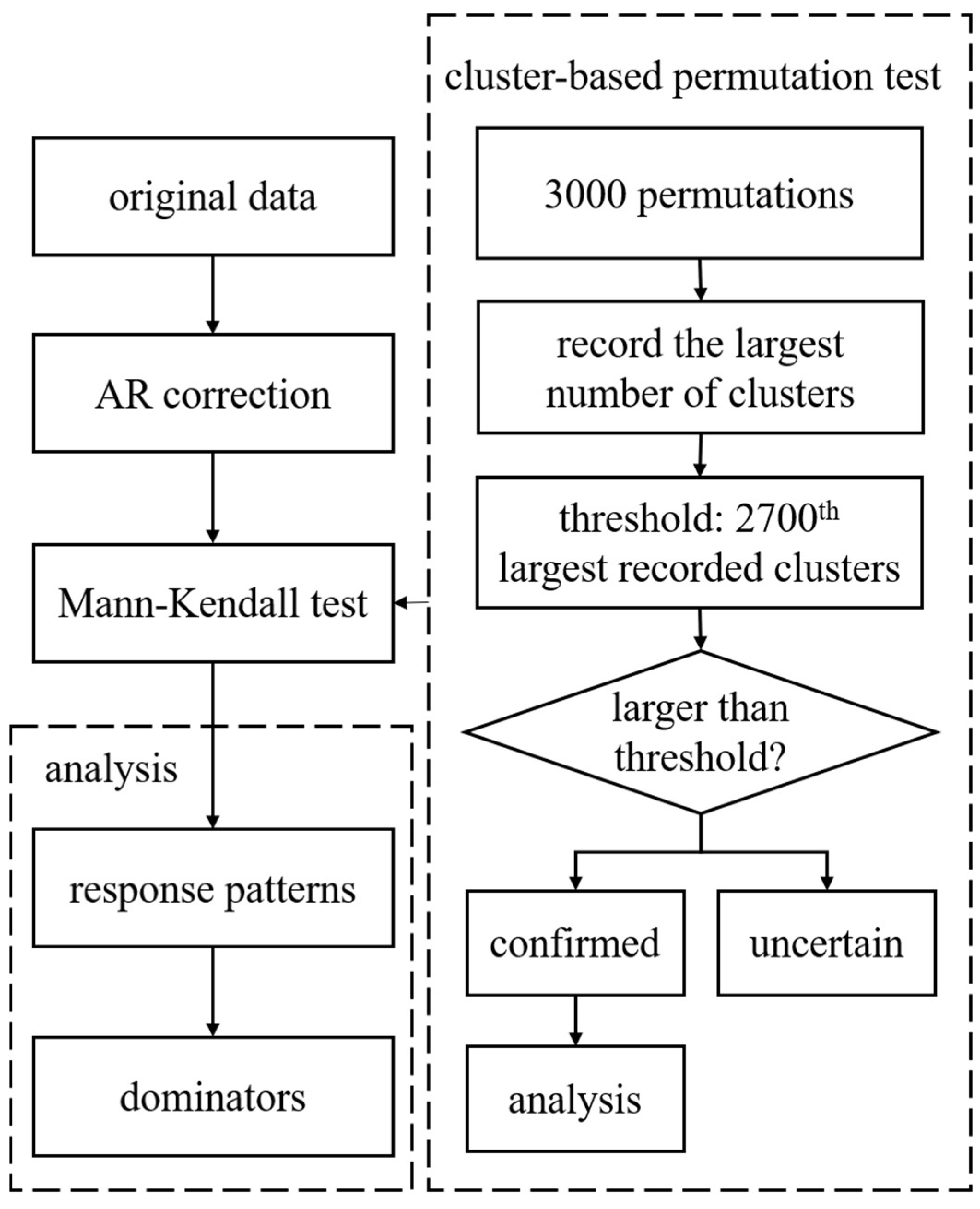
To correct for multiple hypothesis testing, a clustering-based permutation method was applied (Figure 1). The permutation test established a threshold for overall significance based on the number of contiguous (first-order queen neighbors) significant grid cells. The motivation for this test was that the clusters formed by false positives were smaller than those formed when a true increase or decrease in WY existed. A total of 3000 permutations were performed to determine the threshold for statistical significance. At each permutation, all grid cells were permuted jointly, that is, using the same set of permuted time indices. This preserves the spatial correlation of the data. The MK trend test was performed on the permuted data, and the largest cluster of significant grid cells was recorded. The 2700th of the 3000 largest recorded clusters (i.e., 90th percentile) was the threshold for overall significance. In the original data, the number of grid cells for each significant region was counted, and if it exceeded the threshold established by the permutation method, it was declared that this region had a confirmed change. This method has been proven to control the probability of false positives in the results and has higher statistical power than comparable methods [31].
For the grid cells with a confirmed significant change in WY, the response patterns of WY to precipitation and ET were identified according to the relationships of their Sen’s slopes. Theil–Sen’s slope estimation is usually used to calculate trend values with MK test. That is, Sen’s slope is first calculated, and then the MK test is used to determine the trend significance. This method is computationally efficient, insensitive to measurement errors and outlier data, and is often used in trend analysis of long time series data [28,46]. Here, six response patterns were defined as follows: SWY+, SP+, and SET+ (Pattern Ⅰ); SWY+, SP+, and SET− (Pattern Ⅱ); SWY+, SP−, and SET− (Pattern Ⅲ); SWY−, SP−, and SET− (Pattern Ⅳ); SWY−, SP−, and SET+ (Pattern Ⅴ); SWY−, SP+, and SET+ (Pattern Ⅵ), where SWY+, SP, and SET stand for the Sen’s slope of WY, precipitation, and ET, respectively.
Based on these six patterns, the dominant component leading to the variation in WY was explored. For precipitation and ET varying in the same direction, that with a large Sen’s slope was taken as the dominant factor. When the two were different, the one with a significant sign was considered the dominant factor. If both were significant, precipitation and ET were considered to act together in WY, whereas if neither were significant, they were set to be determined.
3. Results
3.1. Annual WY at the Global Scale
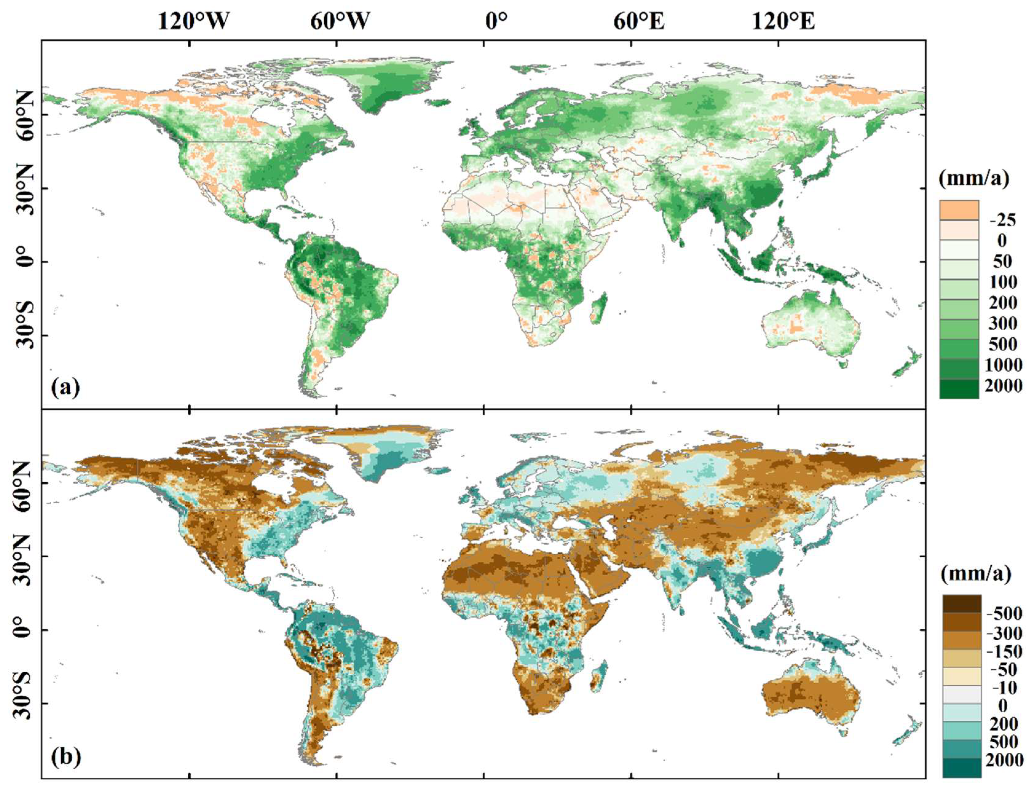
The global 0.5° × 0.5° WY multiyear average (Figure 2a) from 1981 to 2018 was greater than 0 mm in 86.16% of the terrestrial region. In addition, 7.15% of the regions had greater than 1000 mm at 10° S–30° N in eastern Asia, Greenland, and the Amazon basin. The maximum value of 5464.8 mm was located at (77.25°W, 4.25°N). In contrast, 13.84% of the regions had an average WY of less than 0 mm. Among them, 4.82% were less than −500 mm, located on the California Peninsula, the coast of Peru, and the coast of the Arabian Peninsula. The minimum value of −1796.60 mm was located at (115.75°E, 20.25°S). The spatial average of global WY over many years was 299.15 mm/a. The anomalies of 41.59% of the regions with a multi-year average WY greater than 0 mm were greater than 0 mm, while those of all regions with a multi-year average WY of less than 0 mm were less than 0 mm (Figure 2b). There were obvious variations in eastern Asia, Europe, the low-and mid-latitudes of Africa, the mid-latitudes of South America, eastern North America, and mid-to high-latitudes.
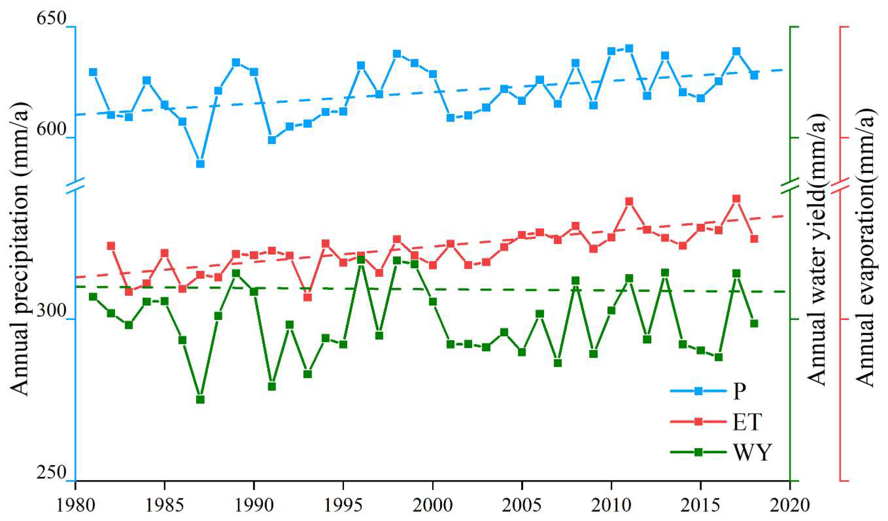
We obtained the annual trends in global land precipitation, ET, and WY from 1981 to 2018 (Figure 3). The results showed that the Sen’s slopes of annual precipitation, ET, and WY were 0.4401, 0.2634, and −0.1188 mm/a, with p-values of 0.0071, 0.00001, and 0.5462 (obtained by the MK test), respectively. The average annual precipitation, ET, and WY were 645.38, 220.50, and 229.15 mm/a. The maximum value of annual precipitation was 665.15 mm/a in 2011, and the minimum value was 616.68 mm/a in 1987. The maximum values occurred in 1981, 1989, and 1996, while the minimum values occurred in 1987, 1991, and 2001. The maximum value of annual ET was 230.52 mm/a in 2016, and the minimum value was 211.33 mm/a in 1992. The maximum annual WY was 318.32 mm/a in 1996, and the minimum value was 275.10 mm/a in 1987. The maximum difference between annual precipitation and ET was 441.35 mm in 1999, and the minimum difference was 401.86 mm in 1987.
3.2. Inter-Annual Variability of WY
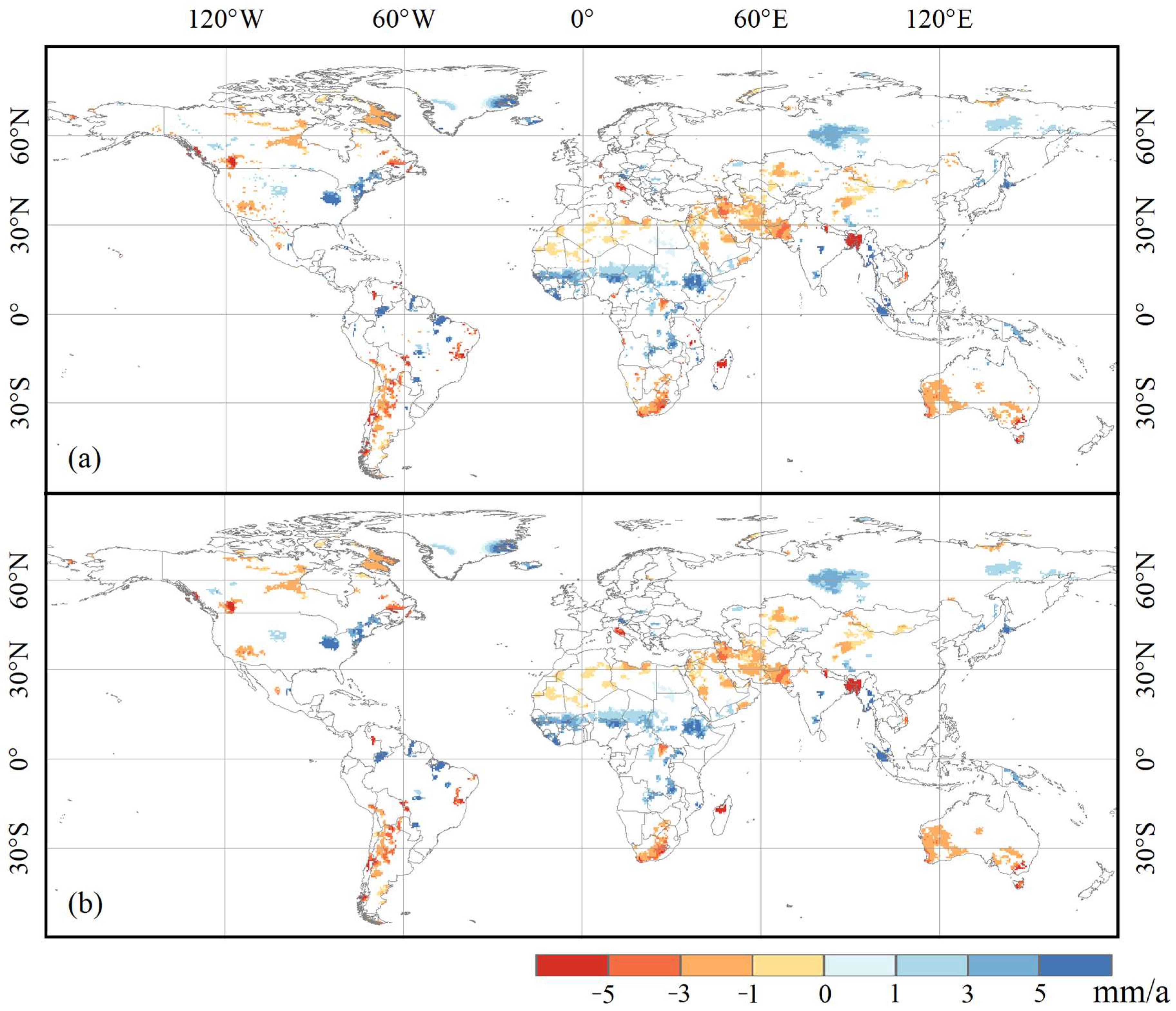
Considering the spatial differences, MK significance tests for each pixel were performed, and 8801 grids with significant changes in global terrestrial WY were obtained (Figure 4a). Not adjusting for multiple hypothesis testing could overestimate the global WY change. Hence, after applying the correction, a confirmed change in 7872 grids was detected (Figure 4b). Areas where there were grids with trend signals that were not strong enough to be detected by the MK method but strong enough to be detected when performing no correction were categorized as uncertain changes. A total of 10.6% of the origin significant changing areas, which are called uncertain changing areas, were screened out after the correction. The mean value of the global terrestrial WY Sen’s slope before the correction was 0.4855, while after the correction, the mean value of the confirmed area was 0.5266 and that of the uncertain area was 0.2496, both showing an overall increasing trend.
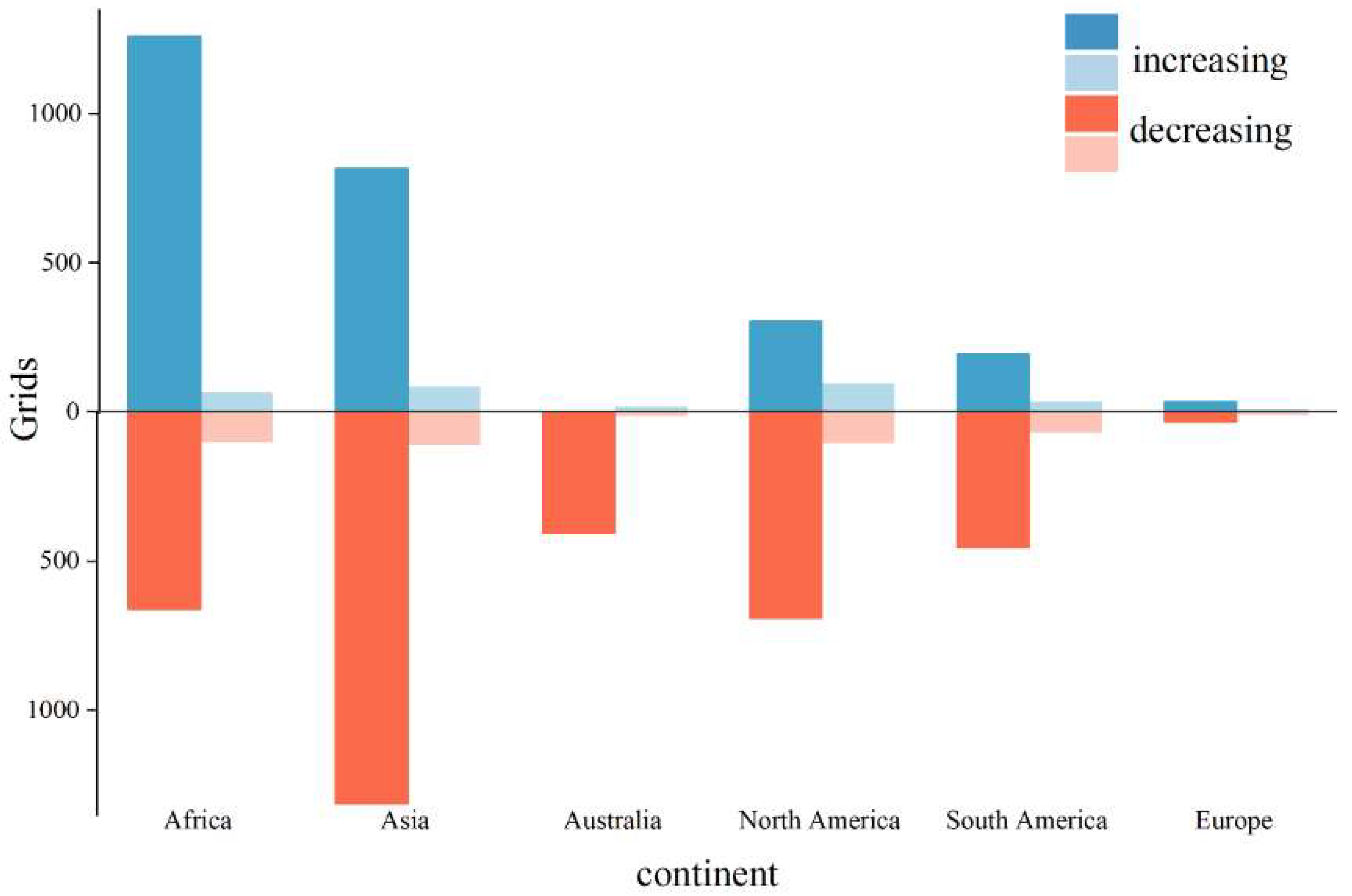
Before applying the correction, 3756 grids (5.72%) showed a significant increasing trend, and 5045 grids (7.68%) showed a significant decreasing trend. After correction, 3361 grids (5.12%) of the global terrestrial WY in the confirmed regions showed an increasing trend, and 4511 grids (6.87%) showed a decreasing trend. The confirmed increasing trend of terrestrial WY in each continent was 48.2% in Africa and 31.3% in Asia, whereas the decreasing trend was 36.8% in Asia, 19.4% in North America, 18.6% in Africa, 12.8% in South America, and 11.5% in Australia. In the uncertain areas of terrestrial WY, 395 grids (0.60%) showed an increasing trend, and 534 grids (0.81%) showed a decreasing trend. Among the increasing trend areas, 30.6% were in North America, and 27.2% were in Asia. Decreasing trends were found in Asia (27.0%), North America (25.3%), and Africa (24.8%) (Figure 5).
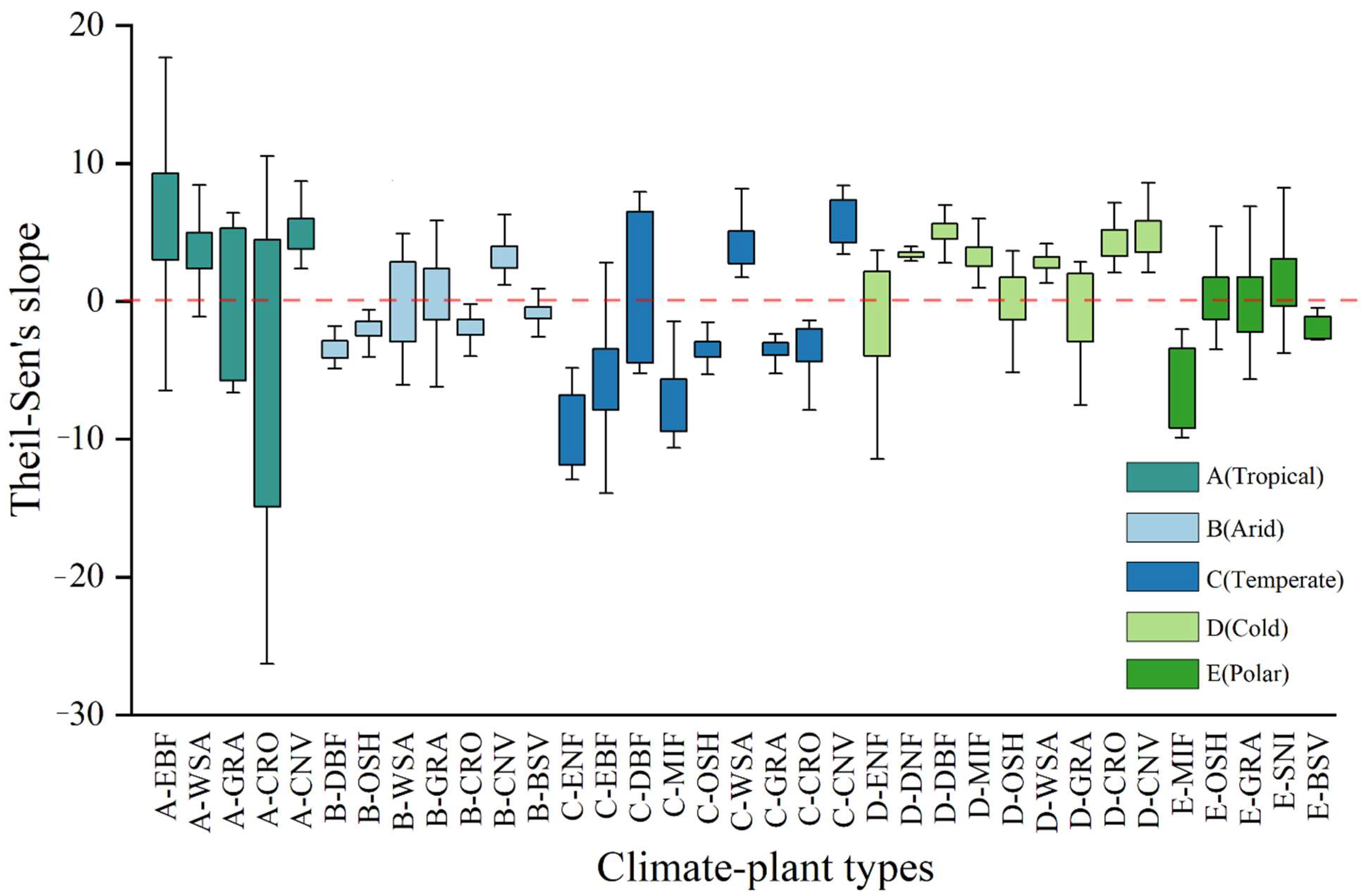
Based on the climate-plant types, the global terrestrial (Figure 6) WY Sen’s slope was positive in EBF, WSA, and CNV in the tropical (A) climate zone, with a significant decrease in WY in CRO and both an increase and a decrease proportionately in GRA. Moreover, WY decreased in DBF, OSH, CRO, and BSV but increased in CNV, and both increased and decreased proportionately in WSA and GRA in the arid (B) climate zone. In the temperate (C) climate zone, WY decreased in ENF, EBF, MIF, OSH, GRA, and CRO, whereas it increased in WSA and CNV, and WY both increased and decreased proportionately in DBF. In the cold (D) climate zone, ENF, OSH, and GRA showed an increased and decreased WY in proportion to each other, while DNF, DBF, MIF, WSA, CRO, and CNV showed an increased WY. In the polar (E) climate zone, WY increased and decreased in OSH and GRA in proportion to each other, while it showed an overall increase in SNI and a decrease in BSV.
3.3. WY in Response to Variabilities of Its Components
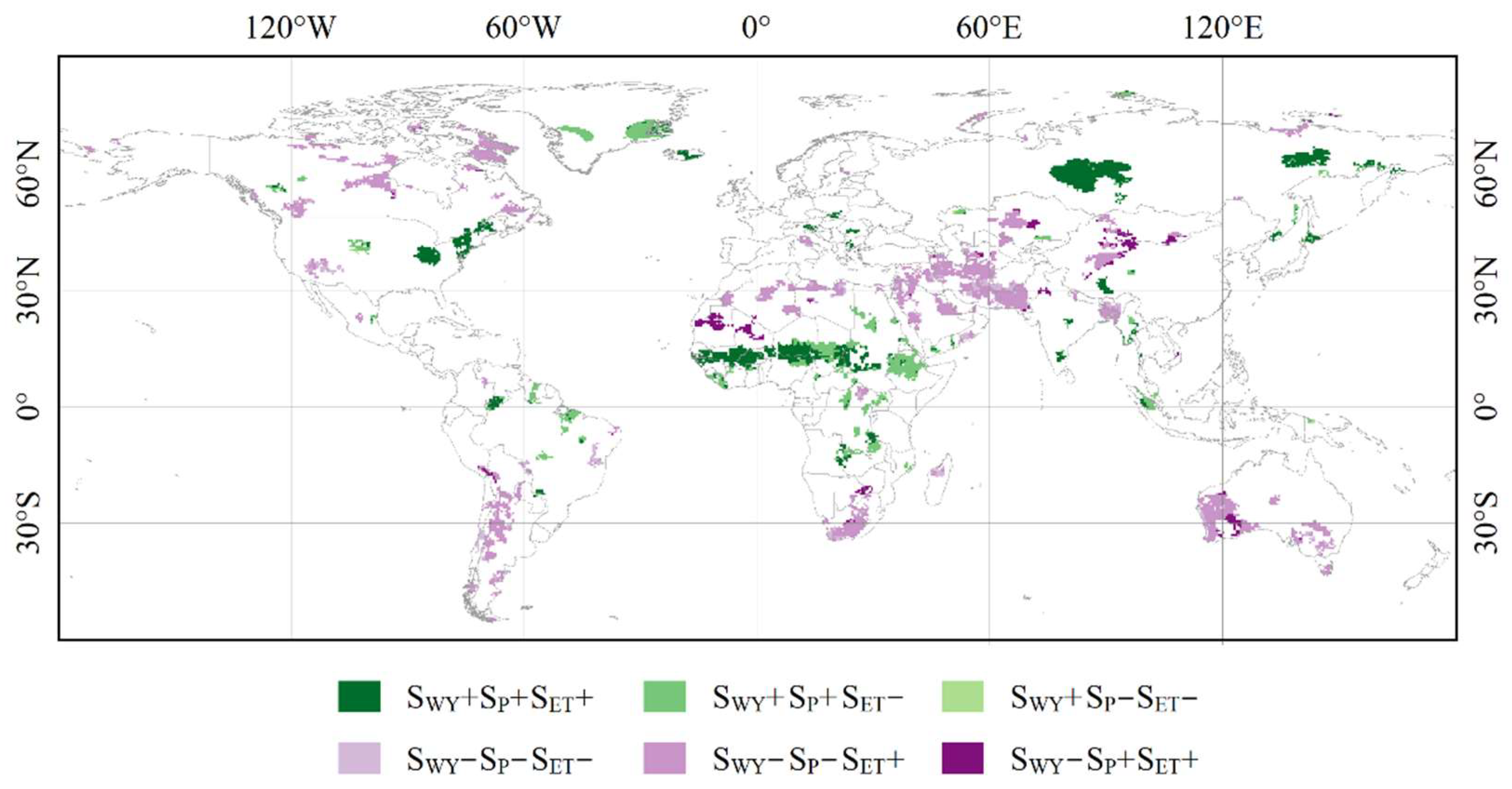
Based on the global terrestrial WY response to precipitation and the ET model (Figure 7), Pattern I (SWY+, SP+, and SET+) was concentrated in Africa and Russia, and Pattern II (SWY+, SP+, and SET−) in Africa. Further, Patterns I (59.3%) and II (40.4%) were widely distributed in the areas with an increasing WY. Pattern IV (SWY−, SP−, and SET−) was scattered around the globe, while Pattern V (SWY−, SP−, and SET+) was more clearly distributed globally, with some parts of North America and southern South America. Additionally, Pattern VI (SWY−, SP+, and SET+) was mainly concentrated in the eastern part of Africa.
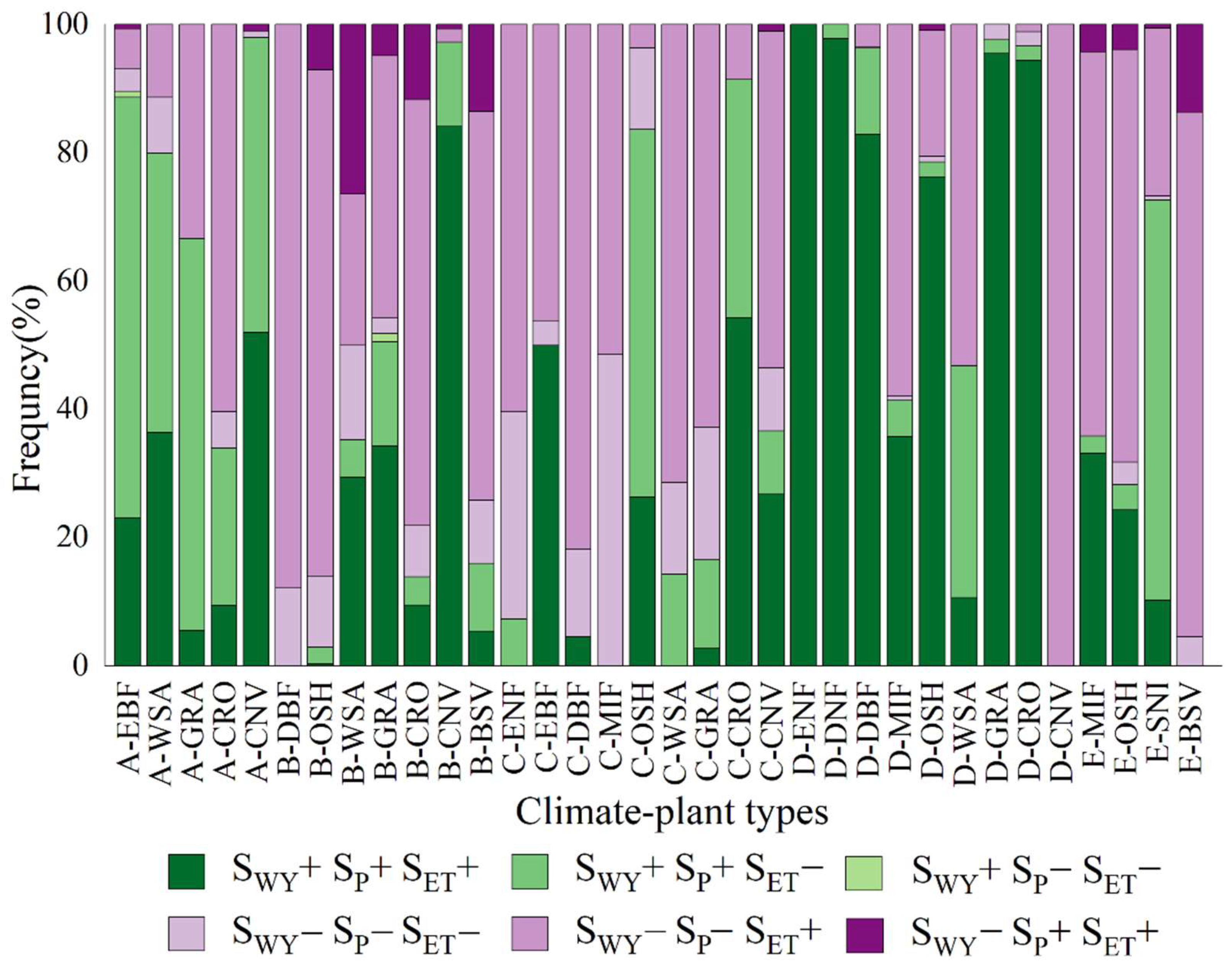
Based on the climate-plant types, the WY response pattern to the variabilities of its components was obtained (Figure 8). Areas in A-CRO, B-CRO, and C-CRO with Pattern V accounted for the majority, whereas the D-CRO was associated with Pattern I. In the MIF of different climate zones, different patterns occupied the following different proportions: C-MIF with Pattern V, D-MIF with Pattern I, and E-MIF with Pattern V. The difference was that the CNV and OSH in different regions showed the same pattern.
3.4. Dominating Factors for the Changes in WY
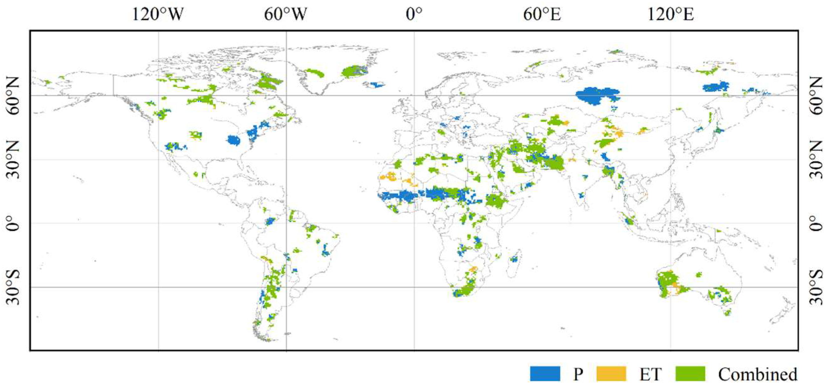
The spatial distribution of the dominant factors of global WY change (Figure 9) showed that the area of the region where WY changes were dominated by precipitation accounted for 31.5% and was distributed in central Africa, North America, and Siberia. The areas dominated by a combination of precipitation and ET accounted for 61.2% and were distributed worldwide. The regions where WY changes were dominated by ET were found on the western side of Africa. The regions with a significant increasing trend in WY were dominated by precipitation (59.2%) and the combined effect (40.4%), while the regions with a significant decreasing trend were mainly dominated by the combined effect (78.4%).
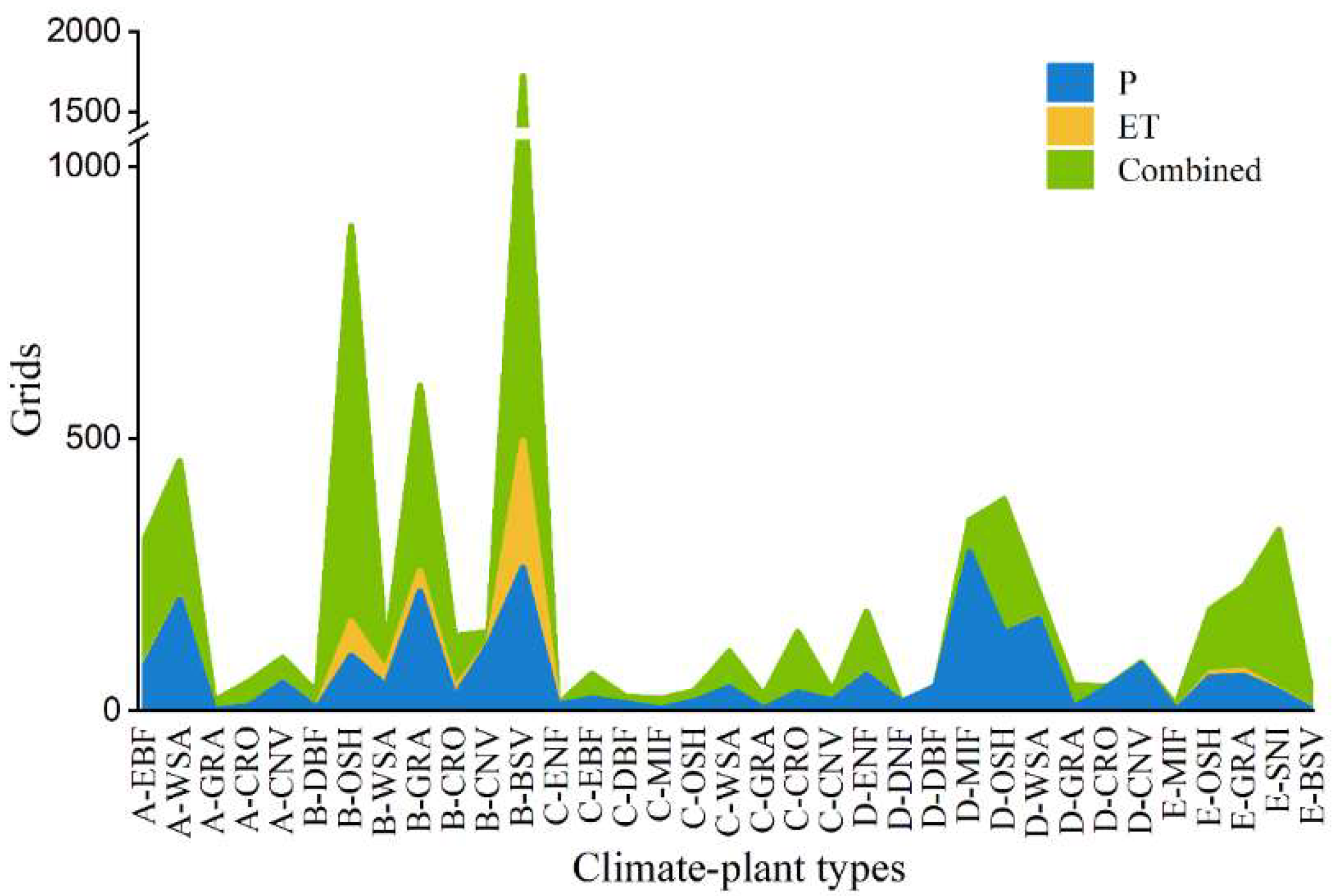
Based on the climate-plant types, the main factors of WY variation were mapped (Figure 10). The WY changes in regions with A-CRO, B-CRO, and C-CRO were dominated by the combined effect, whereas D-CRO was dominated by precipitation. Similarly, C-MIF and E-MIF were dominated by the combined effect, whereas D-MIF was dominated by precipitation. The areas with A-CNV and C-CNV were dominated by precipitation and combined effects, whereas the areas with B-CNV and D-CNV were dominated by precipitation. The OSH in all climate regions was primarily a combined effect.
4. Discussion
Improving the understanding of changes in WY and the dominant drivers is essential for assessing the impact of global climate change on the water cycle. Previous studies have suggested that WY changes due to precipitation and ET in local areas. However, spatiotemporal changes in WY in global terrines and their response patterns to precipitation and ET have not yet been considered. In this study, a new step, correcting for multiple hypothesis testing, was introduced. This study showed that the increasing and decreasing trends in WY have changed around the world. Furthermore, the contribution of the WY change was different in different regions.
The high values of the multi-year average WY were mostly concentrated in coastal areas, while the low values were concentrated inland (Figure 2a). As for the trend of “Dry gets drier, wet gets wetter”, we found (Figure 2b) that WY in all dry regions where multi-year average WY was less than 0 mm/a was decreasing. It was a negative indicator of local water resources [47]. However, for areas that are already rich in WY, it is still necessary to pay attention to the climate change and land cover change to avoid the impact of the decreasing WY somewhere. Some researchers [48] also pointed out that the impact of climate change on global WY was reflected in wet and dry seasons.
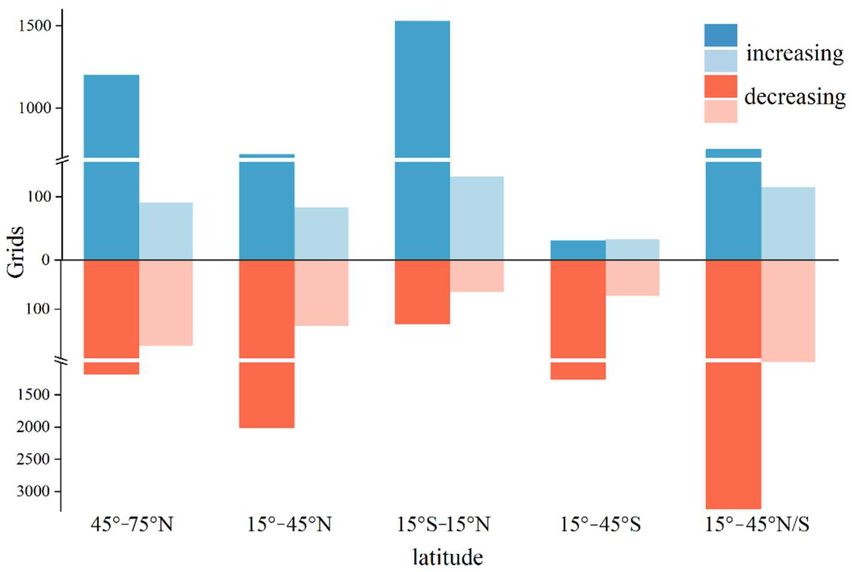
The application of the correction based on clustering corrected the overestimation of the degree of global WY change (Figure 4). After applying the correction, we found that approximately 10% of the global areas that demonstrated a significant change in uncertainty were eliminated. The extent of overestimation can be better understood by examining climate zones and land-use types. The results showed that the uncertain areas were mainly concentrated in non-woody plants, such as open shrublands, closed shrublands, and savannas. Moreover, the number of uncertain grids was relatively high for arid desert, arid steppe, and polar tundra climates. In addition, harsher climates and sparser vegetation were observed. WY was mostly increasing in the tropical zone (15°S–15°N), while an overall decreasing trend was observed near 30°N and 30°S (the global desert strip), respectively. We also found that the area in the arid climate type appeared to have more decreasing WY trends. In addition, it is worth noting that the changes were not symmetrical in the northern and southern hemispheres. At high latitudes in the Northern Hemisphere, both increasing and decreasing trends were observed (Figure 11). These might relate to the global wind belts.
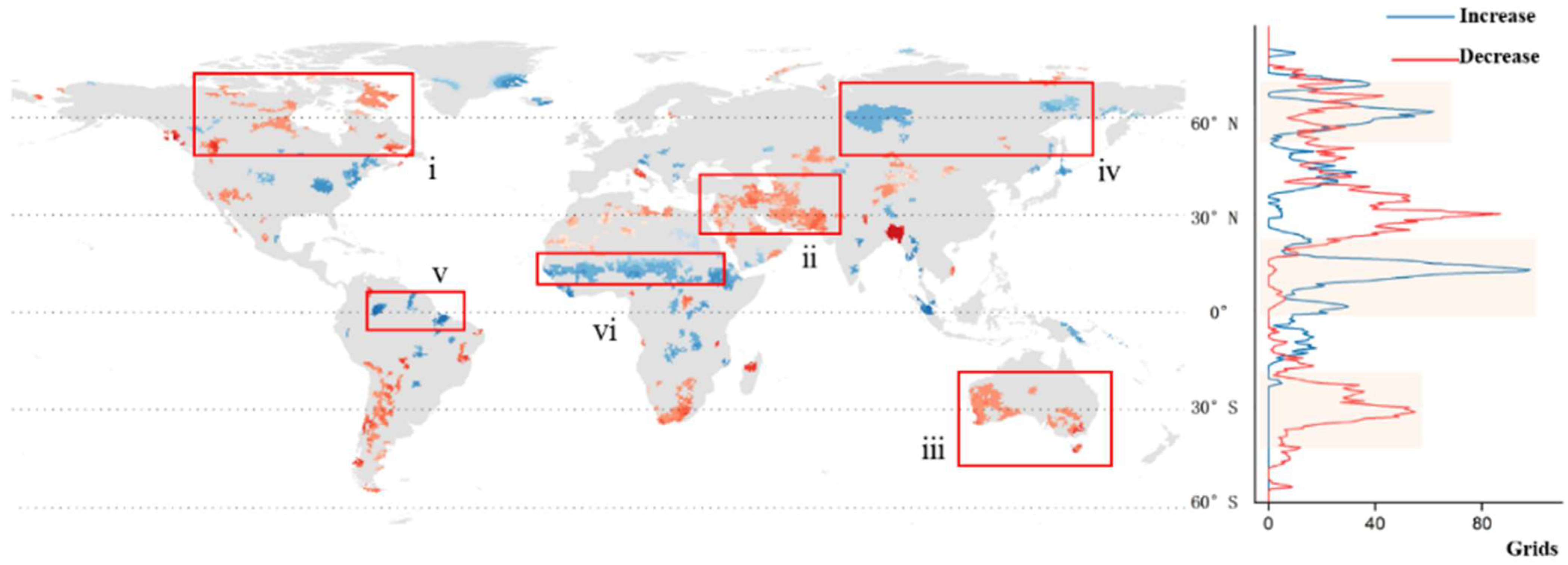
Global terrestrial WY during 1981–2018 showed a fluctuating downward trend (Figure 3). Based on the latitudinal variation map of global terrestrial WY changes (Figure 4), WY at low latitudes was dominated by an increasing trend, that at mid-latitudes in the northern and southern hemispheres was dominated by a decreasing trend, and that at high latitudes in the northern hemisphere had a proportion of increasing and decreasing trends. We selected some typical regions for the discussion (Figure 12). All regions showed a consistent WY increasing or decreasing trend, except central Africa (Figure 13). According to our defined changing patterns and dominators, Canada (Figure 12(ⅰ)) showed a decreasing trend in WY, caused by a decrease in precipitation and ET. Here, the multi-year average WY was 95.96 mm/a, and Sen’s slope was −1.65 mm/a. Li et al. [49] also showed that the most obvious decreasing trend of WY in Canada occurred in the northeastern and southern mountains but was attributed to the decrease in precipitation and increase in ET. The influence of glacier/permanent snowmelt from the Rocky Mountains and permafrost degradation could be the potential factors in Northwest Canada because of global warming [50,51]. In contrast, the decrease in WY in West Asia (Figure 12(ⅱ)) was mainly caused by a combination of decreased precipitation and increased ET. There was a quite low multi-year average WY (25.17 mm/a) where Sen’s slope was −1.57 mm/a. The combination of decreasing precipitation and increasing atmospheric demand led to a significant increase in aridity in many subtropical areas [52]. Shirmohammadi et al. [53] suggested that local land-use changes might have a higher impact on WY than climate change. The conversion of rangeland and farmland to orchards would decrease WY. These land-use changes affect WY by a structural change in the basin due to an increase in infiltration and ET rates [54]. An overall drying trend in Southern Hemisphere semiarid regions has been noted (since the 1950s for SE Australia [55]). In our results, the decrease in WY (Sen’s slope was −2.16 mm/a) was due to decreased precipitation over most of southeastern Australia (Figure 12(ⅲ)). The substantially higher temperatures, which enhanced atmospheric evaporative demand, coupled with below-average precipitation, resulted in a strong region-wide drought throughout the entire southeastern Australia [56]. Moreover, it might be influenced by sea surface temperature and its interactions with the atmosphere [57].
The increase in WY (Sen’s slope was 2.8573 mm/a) in Siberia (Figure 12(ⅳ)) was caused by an increase in precipitation, with a multi-year average WY of 323.94 mm/a. Extra moisture could be redistributed to the surface through large-scale circulation, creating precipitation in downwind regions. Lian et al. [58] suggested that spring moisture input from the strongly greened upstream regions (Europe) with westerly winds helped to maintain positive feedback of summer precipitation in Siberia when it became weaker. This notable teleconnection resulted in a localized increased wetness trend. Remote correlation is also applied to the Amazon region (Figure 12(ⅴ)). In our study, the Amazon region was mostly characterized by an increase in WY due to increased precipitation and a combination of increased precipitation and decreased ET. The multi-year average WY was high (684.60 mm/a), and Sen’s slope was 7.87 mm/a. Warming from the tropical Atlantic during the wet season triggered more latitudinal water vapor. Seasonal precipitation was important for the maintenance of tropical rainforest ecosystems. Seager et al. [59] suggested that the changes in WY induced by rising specific humidity, which accompanied atmospheric warming, were offset by the slowdown of the tropical circulation to some extent. The large area of the 10° N east-west strip-trending region of Africa (Figure 12(ⅵ)) showed a positive value of Sen’s slope in WY, with a multi-year average WY of 276.92 mm/a, mostly due to increased precipitation. The increase in WY was partly caused by an increase in precipitation and a decrease in ET. Possibly, the increase in WY was due to greening locally or an increase in precipitation in the basin. Data in the study by Cortés et al. [60] showed a significant trend of greening in the area north of the equator in Central Africa. On one hand, some studies suggested that deforestation could increase WY [21], while greening decreased WY by increasing ET [61,62]. On the other hand, Makarieva et al. [63] argued that increasing ET could drive water vapor transport by changing atmospheric pressure. The amount of water recovered to the ground depended greatly on the watershed area that is, the larger the geographical area, the higher the recovery potential.
This study had some limitations. First, the land cover change affected the land surface water cycle, ET, and precipitation [64]. In our study, the IGBP for 2001, in the middle of the study period, was selected as the classification map of the surface cover to minimize the impact of land cover changes on data monitoring. Balist et al. [65] studied the changes in the WY of the Sirvan River Basin in Iran from 2013 to 2019. They found that forests decreased and built-up areas increased. Simultaneously, the precipitation decreased, and temperatures increased in this area over a long period. Therefore, they concluded that the effect of these factors on the WY is a complex process. Second, because we only focused on monotonic trends for the whole period, segmentation might have occurred (e.g., increasing first, then decreasing), which led to overall nonlinear changes. Testing such segmented trends while considering multiple hypothesis testing remains to be investigated. Third, some regions were too small to be detected in our study. Therefore, analysis of these smaller areas might reveal previously undetected trends. Fourth, we found that significant clustering surrounds some insignificant grids. Noise in the trend might lead to insignificance because there was no wall-to-wall ground-truth validation. Nevertheless, our study explicitly showed that global terrestrial WY variability is influenced by precipitation and ET, with different regions showing corresponding trends of increasing or decreasing WY. This study provides a reference for how WY variability can be used for local water management in the future.
5. Conclusions
In summary, this study revisited significant changes in the terrestrial WY using an improved MK test and investigated the response patterns of WY to precipitation and ET. The traditional MK test showed that the terrestrial WY changed significantly over 13.4% of continents, whereas 10.6% of which were removed because of their uncertainties in the permutation test. The confirmed increasing trends of WY were located in Africa, eastern North America, and Siberia, whereas the confirmed decreasing trends were concentrated in Asia and Oceania. The dominant factors for the increase in WY were mainly precipitation, while the combined effect of precipitation and ET accounted for most of the significant decreases in WY.
Author Contributions
Software, formal analysis, writing—original draft preparation H.G.; conceptualization, resources, writing—review and editing, J.J. All authors have read and agreed to the published version of the manuscript.
Funding
This research was funded by the National Key R&D Program of China, grant number 2018YFA0605402 and the National Natural Science Foundation of China, grant number 41971374.
Data Availability Statement
Not applicable.
Conflicts of Interest
The authors declare no conflict of interest.
References
- Díaz, M.E.; Figueroa, R.; Alonso, M.L.S.; Vidal-Abarca, M.R. Exploring the complex relations between water resources and social indicators: The Biobío Basin (Chile). Ecosyst. Serv. 2018, 31, 84–92. [Google Scholar] [CrossRef]
- Gleick, P.H. Water and energy. Annu. Rev. Energy Env. 1994, 19, 267–299. [Google Scholar] [CrossRef]
- Tidwell, V.; Moreland, B. Mapping water consumption for energy production around the Pacific Rim. Environ. Res. Lett. 2016, 11, 094008. [Google Scholar] [CrossRef] [Green Version]
- Parkinson, S.; Krey, V.; Huppmann, D.; Kahil, T.; McCollum, D.; Fricko, O.; Byers, E.; Gidden, M.J.; Mayor, B.; Khan, Z.; et al. Balancing clean water-climate change mitigation trade-offs. Environ. Res. Lett. 2019, 14, 014009. [Google Scholar] [CrossRef]
- Sood, M.; Singal, S.K. Development of hydrokinetic energy technology: A review. Int. J. Energy Res. 2019, 43, 5552–5571. [Google Scholar] [CrossRef]
- Haddeland, I.; Heinke, J.; Biemans, H.; Eisner, S.; Flörke, M.; Hanasaki, N.; Konzmann, M.; Ludwig, F.; Masaki, Y.; Schewe, J.; et al. Global water resources affected by human interventions and climate change. Proc. Natl. Acad. Sci. USA 2014, 111, 3251–3256. [Google Scholar] [CrossRef] [Green Version]
- IPCC Climate Change 2021: The Physical Science Basis Contribution of Working Group I to the Sixth Assessment Report of the Intergovernmental Panel on Climate Change; IPCC: Geneva, Switzerland, 2021.
- Liao, X.L.; Xu, W.; Zhang, J.L.; Li, Y.; Tian, Y.G. Global exposure to rainstorms and the contribution rates of climate change and population change. Sci. Total Environ. 2019, 663, 644–656. [Google Scholar] [CrossRef]
- Fu, Q.; Feng, S. Responses of terrestrial aridity to global warming. J. Geo-Phys. Res. Atmos. 2014, 119, 7863–7875. [Google Scholar] [CrossRef]
- Held, I.M.; Soden, B.J. Robust responses of the hydrological cycle to global warming. J. Clim. 2006, 19, 5686–5699. [Google Scholar] [CrossRef]
- Greve, P.; Orlowsky, B.; Mueller, B.; Sheffield, J.; Reichstein, M.; Seneviratne, S.I. Global assessment of trends in wetting and drying over land. Nat. Geosci. 2014, 7, 716–721. [Google Scholar] [CrossRef]
- Wilson, K.B.; Hanson, P.J.; Mulholland, P.J.; Baldocchi, D.D.; Wullschleger, S.D. A comparison of methods for determining forest evapotranspiration and its components: Sap-flow, soil water budget, eddy covariance and catchment water balance. Agric. For. Meteorol. 2001, 106, 153–168. [Google Scholar] [CrossRef]
- Peterson, T.C.; Golubev, V.S.; Groisman, P.Y. Evaporation losing its strength. Nature 1995, 377, 687–688. [Google Scholar] [CrossRef]
- Gong, L.B.; Xu, C.Y.; Chen, D.L.; Halldin, S.; Chen, Y.Q.D. Sensitivity of the Penman-Monteith reference evapotranspiration to key climatic variables in the Changjiang (Yangtze River) basin. J. Hydrol. 2006, 329, 620–629. [Google Scholar] [CrossRef]
- Liu, X.M.; Zheng, H.X.; Zhang, M.H.; Liu, C.M. Identification of dominant climate factor for pan evaporation trend in the Tibetan Plateau. J. Geog. Sci. 2011, 21, 594–608. [Google Scholar] [CrossRef]
- Jackson, R.B.; Jobbágy, E.G.; Avissar, R.; Roy, S.B.; Barrett, D.J.; Cook, C.W.; Farley, K.A.; le Maitre, D.C.; McCarl, B.A.; Murray, B.C. Trading Water for Carbon with Biological Carbon Sequestration. Science 2005, 310, 1944–1947. [Google Scholar] [CrossRef] [PubMed] [Green Version]
- Brown, A.E.; Zhang, L.; McMahon, T.A.; Western, A.W.; Vertessy, R.A. A review of paired catchment studies for determining changes in water yield resulting from alterations in vegetation. J. Hydrol. 2005, 310, 28–61. [Google Scholar] [CrossRef]
- Jiang, B.; Liang, S.L. Improved vegetation greenness increases summer atmospheric water vapor over Northern China. J. Geophys. Res. Atmos. 2013, 118, 8129–8139. [Google Scholar] [CrossRef]
- Zhang, K.; Kimball, J.S.; Nemani, R.R.; Running, S.W.; Hong, Y.; Gourley, J.J.; Yu, Z.B. Vegetation Greening and Climate Change Promote Multidecadal Rises of Global Land Evapotranspiration. Sci. Rep. 2015, 5, 15956. [Google Scholar] [CrossRef]
- Sun, G.; McNulty, S.G.; Lu, J.; Amatya, D.M.; Liang, Y.; Kolka, R.K. Regional annual water yield from forest lands and its response to potential deforestation across the southeastern United States. J. Hydrol. 2005, 308, 258–268. [Google Scholar] [CrossRef]
- Sun, G.; Zhou, G.Y.; Zhang, Z.Q.; Wei, X.H.; Steven, M.; James, V. Potential Water Yield Reduction Due to Forestation Across China. J. Hydrol. 2006, 328, 548–558. [Google Scholar] [CrossRef]
- López-Moreno, J.I.; Vicente-Serrano, S.; Morán-Tejeda, E.; Zabalza, J.; Lorenzo-Lacruz, J.; García-Ruiz, J.M. Impact of climate evolution and land use changes on water yield in the Ebro Basin. Hydrol. Earth Syst. Sci. Discuss. 2011, 7, 2651–2681. [Google Scholar] [CrossRef] [Green Version]
- Lu, N.; Sun, G.; Feng, X.M.; Fu, B.J. Water yield responses to climate change and variability across the North–South Transect of Eastern China (NSTEC). J. Hydrol. 2013, 481, 96–105. [Google Scholar] [CrossRef]
- Yue, S.; Pilon, P.; Phinney, B.; Cavadias, G. The influence of autocorrelation on the ability to detect trend in hydrological series. Hydrol. Processes 2002, 16, 1807–1829. [Google Scholar] [CrossRef]
- Gan, T.Y. Hydroclimatic trends and possible climatic warming in the Canadian Prairies. Water Resour. Res. 1998, 34, 3009–3015. [Google Scholar] [CrossRef]
- Xu, Z.X.; Li, J.Y.; Liu, C.M. Long-term trend analysis for major climate variables in the Yellow River basin. Hydrol. Processes 2007, 21, 1935–1948. [Google Scholar] [CrossRef]
- Hamed, K.H. Trend detection in hydrologic data: The Mann-Kendall trend test under the scaling hypothesis. J. Hydrol. 2008, 349, 350–363. [Google Scholar] [CrossRef]
- Wang, H.J.; Dai, J.H.; Rutishauser, T.; Gonsamo, A.; Wu, C.Y.; Ge, Q.S. Trends and Variability in Temperature Sensitivity of Lilac Flowering Phenology. J. Geophys. Res. Biogeosci. 2018, 123, 807–817. [Google Scholar] [CrossRef] [Green Version]
- Ventura, V.; Paciorek, C.J.; Risbey, J.S. Controlling the proportion of falsely rejected hypotheses when conducting multiple tests with climatological data. J. Clim. 2004, 17, 4343–4356. [Google Scholar] [CrossRef] [Green Version]
- Wilks, D.S. On “Field Significance” and the false discovery rate. J. Appl. Meteorol. Clim. 2006, 45, 1181–1189. [Google Scholar] [CrossRef]
- Cortés, J.; Miguel, M.; Markus, R.; Alexander, B. Accounting for multiple testing in the analysis of spatio-temporal environmental data. Environ. Ecol. Stat. 2020, 27, 293–318. [Google Scholar] [CrossRef]
- Harris, I.; Jones, P.D.; Osborn, T.J.; Lister, D.H. Updated high-resolution grids of monthly climatic observations-the CRU TS3.10 Dataset. Int. J. Climatol. 2014, 34, 623–642. [Google Scholar] [CrossRef] [Green Version]
- Harris, I.; Osborn, T.J.; Jones, P.; Lister, D. Version 4 of the CRU TS monthly high-resolution gridded multivariate climate dataset. Sci. Data 2020, 7, 109. [Google Scholar] [CrossRef] [PubMed] [Green Version]
- Pepin, N.C.; Losleben, M.; Hartman, M.; Chowanski, K. A Comparison of SNOTEL and GHCN/CRU Surface Temperatures with Free-Air Temperatures at High Elevations in the Western United States: Data Compatibility and Trends. J. Clim. 2005, 18, 1967–1985. [Google Scholar] [CrossRef]
- Zhao, T.B.; Fu, C.B. Comparison of products from ERA-40, NCEP-2, and CRU with station data for summer precipitation over China. Adv. Atmos. Sci. 2006, 23, 593–604. [Google Scholar] [CrossRef]
- Grotjahn, R.; Huynh, J. Contiguous US summer maximum temperature and heat stress trends in CRU and NOAA Climate Division data plus comparisons to reanalyses. Sci. Rep. 2018, 8, 11146. [Google Scholar] [CrossRef]
- Miralles, D.G.; Holmes TR, H.; De Jeu RA, M.; Gash, J.H.; Meesters, A.G.C.A.; Dolman, A.J. Global land-surface evaporation estimated from satellite-based Observations. Hydrol. Earth Syst. Sci. 2011, 15, 453–469. [Google Scholar] [CrossRef] [Green Version]
- Martens, B.; Miralles, D.G.; Lievens, H.; van der Schalie, R.; de Jeu RA, M.; Fernández-Prieto, D.; Beck, H.E.; Dorigo, W.A.; Verhoest, N.E.C. GLEAM v3: Satellite-based land evaporation and root-zone soil moisture. Geosci. Model Dev. 2017, 10, 1903–1925. [Google Scholar] [CrossRef] [Green Version]
- Köppen, W. Die Wärmezonen der Erde, nach der Dauer der heissen, gemässigten und kalten Zeit und nach der Wirkung der Wärme auf die organische Welt betrachtet. Meteorol. Z. 1884, 1, 215–226. [Google Scholar]
- Kottek, M.; Grieser, J.; Beck, C.; Rudolf Band Rubel, F. World Map of the Köppen-Geiger climate classification updated. Meteorol. Z. 2006, 15, 259–263. [Google Scholar] [CrossRef]
- Channan, S.; Channan Xu, X.Y. Half Degree Global MODIS IGBP Land Cover Types (2001–2012). 2018. Available online: http://poles.tpdc.ac.cn/en/data (accessed on 18 March 2022).
- Friedl, M.A.; Sulla-Menashe, D.; Bin Tan Schneider, A.; Ramankutty, N.; Sibley, A.; Huang, X.M. MODIS Collection 5 global land cover: Algorithm refinements and characterization of new datasets. Remote Sens. Environ. 2010, 114, 168–182. [Google Scholar] [CrossRef]
- Beck, H.E.; Zimmermann, N.E.; McVicar, T.R.; Vergopolan, N.; Berg, A.; Wood, E.F. Present and future Köppen-Geiger climate classification maps at 1-km resolution. Sci. Data 2018, 5, 180214. [Google Scholar] [CrossRef] [PubMed] [Green Version]
- Mann, H.B. Nonparametric Tests Against Trend. Econometrica 1945, 13, 245. [Google Scholar] [CrossRef]
- Von Storch, H. Misuses of statistical analysis in climate research Analysis of climate variability. In Analysis of Climate Variability; von Storch, H., Navarra, A., Eds.; Springer: Berlin, Germany, 1999; pp. 11–26. [Google Scholar]
- Fernandes, R.; Leblanc, S.G. Parametric (modified least squares) and non-parametric (Theil–Sen) linear regressions for predicting biophysical parameters in the presence of measurement errors. Remote Sens. Environ. 2005, 95, 303–316. [Google Scholar] [CrossRef]
- Liu, F.; Chen, S.L.; Dong, P.; Peng, J. Spatial and temporal variability of water discharge in the Yellow River Basin over the past 60 years. J. Geogr. Sci. 2012, 22, 1013–1033. [Google Scholar] [CrossRef]
- Konapala, G.; Mishra, A.K.; Wada, Y.; Mann, M.E. Climate change will affect global water availability through compounding changes in seasonal precipitation and evaporation. Nat. Commun. 2020, 11, 3044. [Google Scholar] [CrossRef]
- Li, Z.Q.; Wang, S.S. Water yield variability and response to climate change across Canada. Hydrol. Sci. J. 2021, 66, 1169–1184. [Google Scholar] [CrossRef]
- Walvoord, M.A.; Striegl, R.G. Increased groundwater to stream discharge from permafrost thawing in the Yukon River basin: Potential impacts on lateral export of carbon and nitrogen. Geo-Phys. Res. Lett. 2007, 34, 12. [Google Scholar] [CrossRef] [Green Version]
- Wang, S. Freezing temperature controls winter water discharge for cold region watershed. Water Resour. Res. 2019, 55, 10479–10493. [Google Scholar] [CrossRef] [Green Version]
- Greve, P.; Seneviratne, S.I. Assessment of future changes in water availability and aridity. Geo-Phys. Res. Lett. 2015, 42, 5493–5499. [Google Scholar] [CrossRef] [Green Version]
- Shirmohammadi, B.; Malekian, A.; Salajegheh, A.; Taheri, B.; Azarnivand, H.; Malek, Z.; Verburg, P.H. Impacts of future climate and land use change on water yield in a semiarid basin in Iran Land. Degrad. Dev. 2020, 31, 1252–1264. [Google Scholar] [CrossRef]
- Khazaei, B.; Khatami, S.; Alemohammad, S.H.; Rashidi, L.; Wu, C.; Madani, K.; Aghakouchak, A. Climatic or regionally induced by humans? Tracing hydro-climatic and land-use changes to better understand the Lake Urmia tragedy. J. Hydrol. 2019, 569, 203–217. [Google Scholar] [CrossRef]
- Cai, W.; Cowan, T. Southeast Australia autumn rainfall reduction: A climate-change-induced poleward shift of ocean–atmosphere circulation. J. Clim. 2013, 26, 189–205. [Google Scholar] [CrossRef]
- Ma, X.L.; Huete, A.; Moran, S.; Ponce-Campos, G.; Eamus, D. Abrupt shifts in phenology and vegetation productivity under climate extremes. J. Geophys. Res. Biogeosci. 2015, 120, 2036–2052. [Google Scholar] [CrossRef]
- Khaledi, J.; Nitschke, C.; Lane PN, J.; Penman, T.; Nyman, P. The influence of atmosphere-ocean phenomenon on water availability across temperate Australia. Water Resour. Res. 2022, 58, e2020WR029409. [Google Scholar] [CrossRef]
- Lian, X.; Piao, S.L.; Li LZ, X.; Li, Y.; Huntingford, C.; Ciais, P.; Cescatti, A.; Janssens, I.A.; Peñuelas, J.; Buermann, W.; et al. Summer soil drying exacerbated by earlier spring greening of northern vegetation. Sci. Adv. 2020, 6, eaax0255. [Google Scholar] [CrossRef] [PubMed] [Green Version]
- Seager, R.; Naik, N.; Vecchi, G.A. Thermodynamic and dynamic mechanisms for large-scale changes in the hydrological cycle in response to global warming. J. Clim. 2010, 23, 4651–4668. [Google Scholar] [CrossRef] [Green Version]
- Cortés, J.; Mahecha, M.D.; Reichstein, M.; Myneni, R.B.; Chen, C.; Brenning, A. Where Are Global Vegetation Greening and Browning Trends Significant? Geophys. Res. Lett. 2021, 48, e2020GL091496. [Google Scholar] [CrossRef]
- Liu, Y.B.; Xiao, J.F.; Ju, W.M.; Xu, K.; Zhou, Y.L.; Zhao, Y.T. Recent trends in vegetation greenness in China significantly altered annual evapotranspiration and water yield. Environ. Res. Lett. 2016, 11, 094010. [Google Scholar] [CrossRef]
- Zhang, J.H.; Zhang, Y.L.; Sun, G.; Song, C.H.; Dannenberg, M.P.; Li, J.F.; Liu, N.; Zhang, K.R.; Zhan, Q.F.; Hao, L. Vegetation greening weakened the capacity of water supply to China’s South-to-North Water Diversion Project. Hydrol. Earth Syst. Sci. 2021, 25, 5623–5640. [Google Scholar] [CrossRef]
- Makarieva, A.M.; Gorshkov, V.G. Biotic pump of atmospheric moisture as driver of the hydrological cycle on land. Hydrol. Earth Syst. Sci. 2007, 11, 1013–1033. [Google Scholar] [CrossRef] [Green Version]
- Zhang, L.; Chen, L.; Chiew, F.; Fu, B.J. Understanding the impacts of climate and landuse change on water yield. Curr. Opin. Env. Sust. 2018, 33, 167–174. [Google Scholar] [CrossRef]
- Balist, J.; Malekmohammadi, B.; Jafari, H.R.; Nohegar, A.; Geneletti, D. Detecting land use and climate impacts on water yield ecosystem service in arid and semi-arid areas. A study in Sirvan River Basin-Iran. Appl. Water Sci. 2022, 12, 4. [Google Scholar] [CrossRef]
Figure 1.
The framework of the whole methodology.

Figure 2.
Geographic distribution of (a) the multi-year average values of annual terrestrial water yield during 1981−2018 and (b) its spatial anomalies.
Figure 2.
Geographic distribution of (a) the multi-year average values of annual terrestrial water yield during 1981−2018 and (b) its spatial anomalies.

Figure 3.
Temporal variabilities of annual terrestrial water yield (WY), precipitation (P), and evapotranspiration (ET) globally from 1981 to 2018. The colored dots and dash lines denote the yearly average values and the linear trends of the variables, respectively.
Figure 3.
Temporal variabilities of annual terrestrial water yield (WY), precipitation (P), and evapotranspiration (ET) globally from 1981 to 2018. The colored dots and dash lines denote the yearly average values and the linear trends of the variables, respectively.

Figure 4.
Geographic distribution of significant trends in annual terrestrial water yield during 1981−2018, using the Mann-Kendal trend test, (a) before and (b) after correcting for multiple hypothesis testing. Shades of blue (red) indicate a significant increasing (decreasing) trend at α = 0.05. Grid cells with no statistical significance are shown in white.

Figure 5.
Significant changes in annual terrestrial water yield according to the number of grid cells globally. Darker shades indicate the confirmed increasing (decreasing) trends that remains after correcting for multiple hypothesis testing (α = 0.05), while lighter shades indicate the uncertain trends, i.e., additional significant changes that are detected when no multiple testing correction took place.

Figure 6.
The Theil–Sen’s slope showing the confirmed trends in annual terrestrial water yield (WY) according to the climate-plant types, which are defined by Köppen-Geiger (KG) climate zones vs. IGBP land cover type (Table 1). The box plots show lower bound (=Q1 − 1.5 LQR), lower quartile (Q1), upper quartile (Q3) and upper bound (=Q3 + 1.5 LQR) from bottom to top, where LQR = Q3 − Q1.

Figure 7.
Composite map of the sign of terrestrial water yield (WY), precipitation (P), and evapotranspiration (ET) trends. Colored areas indicate where WY significantly changed during 1981–2018 after correcting for multiple hypothesis testing (α = 0.05). SWY, SP, and SET indicate the Theil–Sen’s slope of WY, P, and ET, respectively. The symbols + and − indicate a positive and negative WY (P or ET) trend during the study period, respectively.

Figure 8.
Frequency distribution of composite patterns of terrestrial water yield (WY), precipitation (P), and evapotranspiration (ET) trends by the climate-plant types (shown in Figure 6) across the grid cells in which WY significantly changed during 1981–2018 after correcting for multiple hypothesis testing (α = 0.05). SWY, SP, and SET indicate the Theil–Sen’s slope of WY, P, and ET, respectively. The symbols + and − indicate a positive and negative WY (P or ET) trend during the study period, respectively.

Figure 9.
Geographic distribution of dominators regulating terrestrial water yield (WY). Colored areas indicate those where WY significantly changed during 1981–2018 after correcting for multiple hypothesis testing (α = 0.05). Blue, yellow, and green indicate that WY was dominated by precipitation (P), evapotranspiration (ET), and their combined effect (Combined), respectively.

Figure 10.
Statistics for the dominating factors regulating terrestrial water yield (WY) by the climate-plant types (Figure 5) across the grid cells in which WY significantly changed during 1981–2018 after correcting for multiple hypothesis testing (α = 0.05). Blue, yellow, and green indicate that WY was dominated by precipitation (P), evapotranspiration (ET), and their combined effect (Combined), respectively.

Figure 11.
Significant changes in annual terrestrial water yield according to the number of grid cells in different altitude. Darker shades indicate the confirmed increasing (decreasing) trends that remains after correcting for multiple hypothesis testing (α = 0.05), while lighter shades indicate the uncertain trends, i.e., additional significant changes that are detected when no multiple testing correction took place.

Figure 12.
Statistics for the confirmed trends of terrestrial water yield (WY) represented as the number of grid cells by the latitude. Blue and red indicate a significant increase and decrease in WY during 1981–2018 after correcting for multiple hypothesis testing (α = 0.05), respectively. The red boxes indicate the areas of interest, including parts of Canada (i), West Asia (ii), Australia (iii), Siberia (iv), the Amazon (v), and Central Africa (vi).

Figure 13.
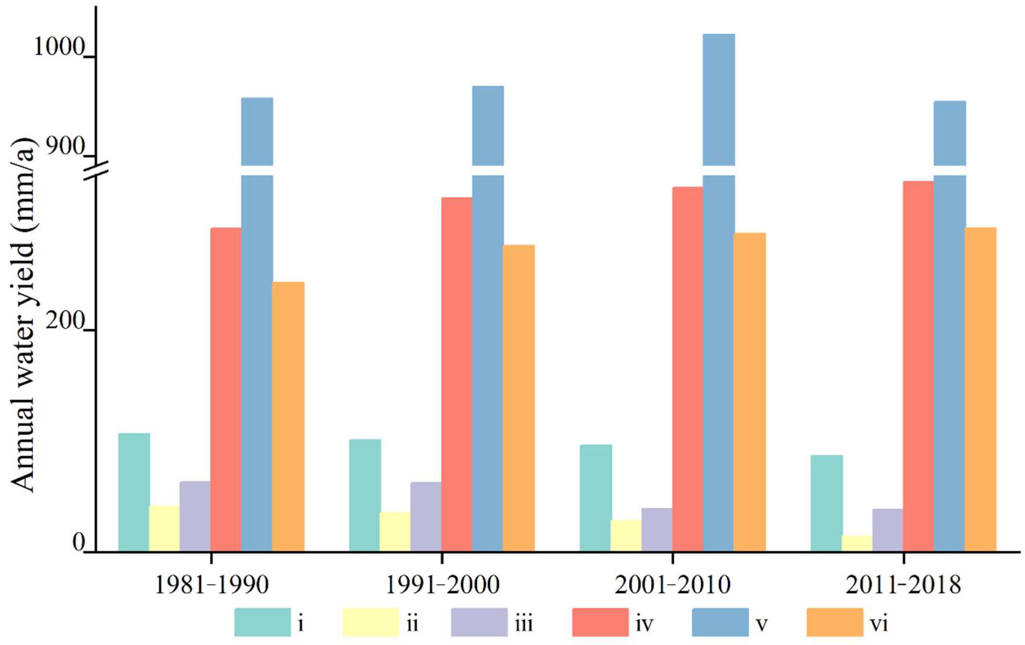
Temporal variabilities of ten-year average terrestrial water yield (WY) from 1981 to 2018 in typical regions (Figure 12). The colored boxes indicate the areas of interest, including parts of Canada (i), West Asia (ii), Australia (iii), Siberia (iv), the Amazon (v), and Central Africa (vi).
Figure 13.
Temporal variabilities of ten-year average terrestrial water yield (WY) from 1981 to 2018 in typical regions (Figure 12). The colored boxes indicate the areas of interest, including parts of Canada (i), West Asia (ii), Australia (iii), Siberia (iv), the Amazon (v), and Central Africa (vi).

Publisher’s Note: MDPI stays neutral with regard to jurisdictional claims in published maps and institutional affiliations. |
© 2022 by the authors. Licensee MDPI, Basel, Switzerland. This article is an open access article distributed under the terms and conditions of the Creative Commons Attribution (CC BY) license (https://creativecommons.org/licenses/by/4.0/).
Share and Cite
MDPI and ACS Style
Gao, H.; Jin, J. Analysis of Water Yield Changes from 1981 to 2018 Using an Improved Mann-Kendall Test. Remote Sens. 2022, 14, 2009. https://0-doi-org.brum.beds.ac.uk/10.3390/rs14092009
AMA Style
Gao H, Jin J. Analysis of Water Yield Changes from 1981 to 2018 Using an Improved Mann-Kendall Test. Remote Sensing. 2022; 14(9):2009. https://0-doi-org.brum.beds.ac.uk/10.3390/rs14092009
Chicago/Turabian StyleGao, Han, and Jiaxin Jin. 2022. "Analysis of Water Yield Changes from 1981 to 2018 Using an Improved Mann-Kendall Test" Remote Sensing 14, no. 9: 2009. https://0-doi-org.brum.beds.ac.uk/10.3390/rs14092009
Note that from the first issue of 2016, this journal uses article numbers instead of page numbers. See further details here.