
Intercomparison of Real and Simulated GEDI Observations across Sclerophyll Forests


1
Remote Sensing Centre, Geospatial Science, School of Science, RMIT University, 402 Swanston Street, Melbourne 3000, Australia
2
New South Wales Department of Primary Industries, 4 Parramatta Square, Parramatta 2150, Australia
*
Author to whom correspondence should be addressed.
Remote Sens. 2022, 14(9), 2096; https://0-doi-org.brum.beds.ac.uk/10.3390/rs14092096
Submission received: 21 March 2022
/
Revised: 14 April 2022
/
Accepted: 19 April 2022
/
Published: 27 April 2022
(This article belongs to the Topic Remote Sensing and Geoinformatics in Agriculture and Environment)
Abstract
:Forest structure is an important variable in ecology, fire behaviour, and carbon management. New spaceborne lidar sensors, such as the Global Ecosystem Dynamics Investigation (GEDI), enable forest structure to be mapped at a global scale. Virtual GEDI-like observations can be derived from airborne laser scanning (ALS) data for given locations using the GEDI simulator, which was a tool initially developed for GEDI’s pre-launch calibration. This study compares the relative height (RH) and ground elevation metrics of real and simulated GEDI observations against ALS-derived benchmarks in southeast Australia. A total of 15,616 footprint locations were examined, covering a large range of forest types and topographic conditions. The impacts of canopy cover and height, terrain slope, and ALS point cloud density were assessed. The results indicate that the simulator produces more accurate canopy height (RH95) metrics (RMSE: 4.2 m, Bias: −1.3 m) than the actual GEDI sensor (RMSE: 9.6 m, Bias: −1.6 m). Similarly, the simulator outperforms GEDI in ground detection accuracy. In contrast to other studies, which favour the Gaussian algorithm for ground detection, we found that the Maximum algorithm performed better in most settings. Despite the determined differences between real and simulated GEDI observations, this study indicates the compatibility of both data sources, which may enable their combined use in multitemporal forest structure monitoring.
1. Introduction
Forests are key ecosystems, hosting a large proportion of earth’s plant species [1], and playing an essential role in climate change mitigation [2]. One factor that determines a forest’s value for biodiversity and its role as a carbon sink is its vertical structure [3,4]. Research has shown that ecosystem functions and species richness depend on the vertical arrangement of plant material [4,5]. Furthermore, information on vertical forest structure enables the modelling of biomass and related variables [6,7,8,9], which is essential for monitoring carbon cycles in the interest of climate change mitigation [10].
To obtain information of vertical forest structure at regional and global scales, a growing range of spaceborne remote sensing instruments are available. Passive multispectral sensors provide wall-to-wall imagery on forest dynamics at regular time intervals, with the Landsat archive reaching back as far as 1972. To identify meaningful trends of forest dynamics in these data archives, time series analysis tools such as LandTrendr have been developed [11], exploiting the trajectories of spectral vegetation indices [12]. For instance, the Normalised Burn Ratio (NBR) index relies on the short wave infrared (SWIR) band, which has been demonstrated to be relatively sensitive to forest structure [13]. However, multispectral satellite data archives have limitations in monitoring forest structure for closed-canopy forests due to signal saturation [14].
Active remote sensing technologies, on the other hand, are able to penetrate forest canopies and obtain accurate measurements of the vertical distribution of plant material [15,16]. Light detection and ranging (lidar) has become widely used to gather information about the three-dimensional structure of vegetation, with sensors deployed on terrestrial [17], airborne [18,19], and most recently spaceborne platforms [20]. The ICESat mission carried the first spaceborne lidar system, operating from 2003 to 2009. Despite its focus on measuring ice shields and cloud heights, its data have been successfully used to derive measurements of vertical forest structure [8,21,22]. Since 2019, the Global Ecosystem Dynamics Investigation (GEDI) mission onboard the International Space Station (ISS) has provided data on forest structure over the Earth’s tropical and temperate forests [20].
Sensors such as ICESat, its successor ICESat-2, and GEDI do not provide wall-to-wall information but rather act as sampling tools to provide observations of forest structure at a footprint level. However, their data have been shown to improve the modelling of vertical structure when used in conjunction with wall-to-wall data from multispectral or Synthetic Aperture Radar (SAR) sensors [7,9]. Recent approaches have predicted canopy height and vertical structure over large areas using a combination of Landsat and GEDI [23,24] or Landsat, ICESat, and SAR [22]. Other research evaluated GEDI’s capabilities to estimate aboveground biomass (AGB) using simulated GEDI data [9,25], partly in combination with Landsat imagery [26]. Sanchez-Lopez et al. [15] predicted the time since the last stand-replacing disturbance, and Marselis et al. [4] modelled species richness in tropical forests using simulated large-footprint full waveform lidar.
These studies have successfully demonstrated the advantage of integrating spaceborne lidar data into wall-to-wall forest structural mapping. Nearly all approaches have relied on single-date spaceborne lidar observations. However, forests are dynamic systems subject to various change agents and disturbance events. Thus, it has been proposed to use (spaceborne) lidar observations from multiple epochs to improve the monitoring of forest structural change [27]. This can be particularly beneficial when using lidar observations from both before and after a disturbance event. Although several recent studies have begun to explore the potential of bitemporal spaceborne lidar observations [27,28,29], more studies need to be carried out to further understand the opportunities of using bitemporal lidar observations.
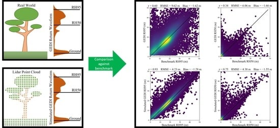
Due to the orbit of the ISS, GEDI’s coverage is limited to latitudes between 51.6°N and 51.6° Slatitude. The sensor is predicted to produce about 10 billion cloud-free observations during its mission, which was initially scheduled for two years. Its three geodetic-class lasers are split (one beam) and dithered after emission, resulting in four full-power and four coverage beams. Each beam results in a transect of footprints on the ground, with 60 m between beam footprints and 600 m between adjacent beam tracks. The nominal diameter of a footprint is 25 m [30]. GEDI’s Level 1B (L1B) product provides geolocated waveform data at the footprint level, whereas L2A data offers ground elevation and relative height (RH) metrics derived from the full returned waveform [20].
Some recent studies relied on simulated GEDI observations due to the limited extent of available GEDI data [9,15,25,26,27]. The GEDI simulator is a tool that was created for the pre-launch calibration of the GEDI instrument. Based on an approach developed by Blair and Hofton [31], the simulator creates virtual waveform observations for given footprint locations using point cloud data, aiming to emulate the data acquisition characteristics of the GEDI sensor [32]. Typically, point clouds from airborne laser scanning (ALS) are used for the simulation [7,25,26].
The GEDI simulator has been validated in various locations in the United States, Costa Rica, and Gabon by intercomparison to large-footprint full waveform lidar observations acquired by the Land, Vegetation and Ice Sensor (LVIS) [32]. However, an independent validation of the GEDI simulator against real GEDI observations has not been undertaken. Furthermore, the simulator’s ability to accurately simulate GEDI observations in Australian sclerophyll vegetation has not been sufficiently evaluated.
Real GEDI data do not allow for multitemporal analysis of forest structure, as it is unlikely that any given footprint location is sampled more than once. However, the GEDI simulator has been proposed as a tool to overcome this limitation and enable bitemporal observation of forest structure [27,28], provided that sufficient ALS data are available for the region of interest. In addition, the GEDI simulator may have potential to serve as a standardisation tool for ALS data sets of different sensors and acquisition parameters, as it has been shown to minimise the influence of flight altitude and pulse density on the virtual waveform [32].
In this paper, the accuracy of both real and simulated GEDI observations is evaluated against ALS baseline data in sclerophyll forests to assess their compatibility for future combined usage. We compare selected RH metrics and ground elevation observations to benchmark metrics derived directly from ALS data across four diverse study sites in southeast Australia. The impact of terrain slope, ALS pulse density, vegetation cover and height is also assessed.
2. Materials and Methods
2.1. Study Area
From all available GEDI Version 2 data, 15,616 footprint locations were selected across four diverse study sites in southeast Australia (Figure 1), named Bendigo, Bright, Canberra and Kosciuszko. The footprints are spread across a variety of forest and terrain types. Elevations within the study area range from 166 to 2036 m and annual rainfall from 460 to 1680 mm. Sclerophyll forests of different canopy cover and height are present across the study sites. Following the definitions used in Australia’s State of the Forests Report [33], eucalypt forests in the study sites were classified as: woodland (canopy cover range 20–50%), open (cover range 50–80%), and closed eucalypt forest (canopy cover above 80%). The height categories Low, Medium, and Tall were assigned to eucalypt forests with a canopy height of less than 10 m, 10–30 m, and above 30 m, respectively. Apart from the various types of eucalypt forest, softwood plantations, rainforest, and other native forests covered parts of the study area (Table 1). The forest type classification was obtained on the footprint level from the Forests of Australia map product [34]. Footprints classified as non-forested were discarded. Slope information was also derived for each footprint according to local, high-resolution digital elevation models (DEM) based on ALS data and classified into seven slope categories, which were binned in 5-degree intervals (Table 2).
2.2. GEDI Data
GEDI L2A data (Version 2) were obtained from the United States’ National Aeronautics and Space Administration (NASA) Earthdata portal for all four study sites and used to extract the geolocation information of all footprints (coordinates of the lowest mode of the waveform) as well as selected metrics of relative height (namely the 50th and 95th relative height percentiles, RH50 and RH95) and ground elevation. All observations were acquired between March 2019 and February 2021. We did not apply any seasonal filtering, as the vertical structure of the investigated evergreen vegetation is not affected by phenological changes in a strictly periodical way [35].
We filtered the GEDI footprints by the quality flag and degrade flag attributes to exclude low-quality observations. Furthermore, we only considered footprint locations that did not experience any type of disturbance after the year 2004 to minimise the impact of disturbance-related vegetation structural change. The disturbance information was derived from multispectral Landsat time series data, which were analysed using the LandTrendr segmentation algorithm [11,36]. The NBR index and an NBR loss threshold of 50 were used for the segmentation, closely following the approach of Nguyen et al. [37], with the sole major variation being the usage of a medoid approach to generate annual composites [38].
2.3. ALS Data
ALS data were used for two purposes: to simulate GEDI observations using the GEDI simulator, and to establish benchmark values (RH and ground elevation metrics) for the intercomparison with the real and simulated GEDI metrics. Publicly available ALS data sets were downloaded from the open data portal Elvis [39]. These data sets originate from aerial campaigns, which have been carried out using a range of ALS sensors and pulse densities (Table 3). All GEDI observations used in this study were acquired between 2019 and 2021, and we ensured all ALS data sets were acquired within four years of that time frame to minimise the effects of forest change. The average ALS point densities across the four study sites ranged from 0.4 to 23 points/m2. We obtained RH benchmark values from the ALS point clouds for all footprint locations using the lidar processing package FUSION [40].
A high-resolution DEM was also obtained for each study site, which was generated from the respective point cloud. The mean DEM elevation within each GEDI footprint served as a benchmark for the intercomparison with GEDI- and simulator-derived ground elevation values. As all DEM data were referenced to the local Australian Height Datum (AHD71), we used a Geoid model to convert the elevation values to ellipsoidal heights, which conform to the vertical datum of GEDI.
2.4. Simulated GEDI Data
Simulated GEDI observations were created for the 15,616 footprint locations. The simulation process consists of two main steps: the first generates a virtual waveform from the ALS data within a given footprint (gediRat tool), and the second derives the GEDI metrics, such as the relative heights and ground elevation, from the simulated waveform (gediMetrics tool) [32]. The simulated RH metrics, along with the actual GEDI observations, were later compared against the benchmark values, which were extracted from the ALS data through FUSION tools [40].
The GEDI simulator provides three different algorithms to determine the ground elevation. The Gaussian method is based on fitting gaussian functions to the simulated waveform to identify the ground return. The Maximum method marks the lowest peak of the simulated waveform as ground signal, whereas the Inflection algorithm derives the ground elevation from the second derivative of the waveform [32]. Thus, the choice of ground detection algorithm has a vital impact on all simulated RH metrics, as these heights are computed in reference to the detected ground elevation.
2.5. Intercomparison
Vertical forest structure can be described using many different metrics. In this study, we focus on RH95, which is a widely used measure of canopy top height [24,28], and RH50, the average height of the footprint [32,44,45].
To assess the performance and compatibility of real and simulated GEDI observations, we compared both data sets against our ALS-derived benchmarks on a footprint level. The assessment included the Pearson correlation coefficient (r), root mean square error (RMSE, Equation (1)), and bias (Equation (2)) of the 50th and 95th percentile RH metrics, as well as the ground elevation metric.
where GEDI can be real or simulated observations of RH95, RH50, or ground elevation, and ALS can be the corresponding metric, respectively, with values derived directly from ALS point cloud data via FUSION tools [40].
For a qualitative investigation of potential error sources, a small number of randomly chosen outliers was examined in detail, using high-resolution aerial imagery (0.1 m) available for the Canberra study site [46]. The results from all three ground detection functions of the GEDI simulator (Gaussian, Maximum, and Inflection algorithm) were assessed, as their performance has a direct impact on the determination of RH metrics. A direct intercomparison of absolute ground elevation metrics between real and simulated GEDI and the ALS-derived DEM was also undertaken.
3. Results
3.1. Performance of GEDI Simulator Algorithms across Different Lidar Point Densities
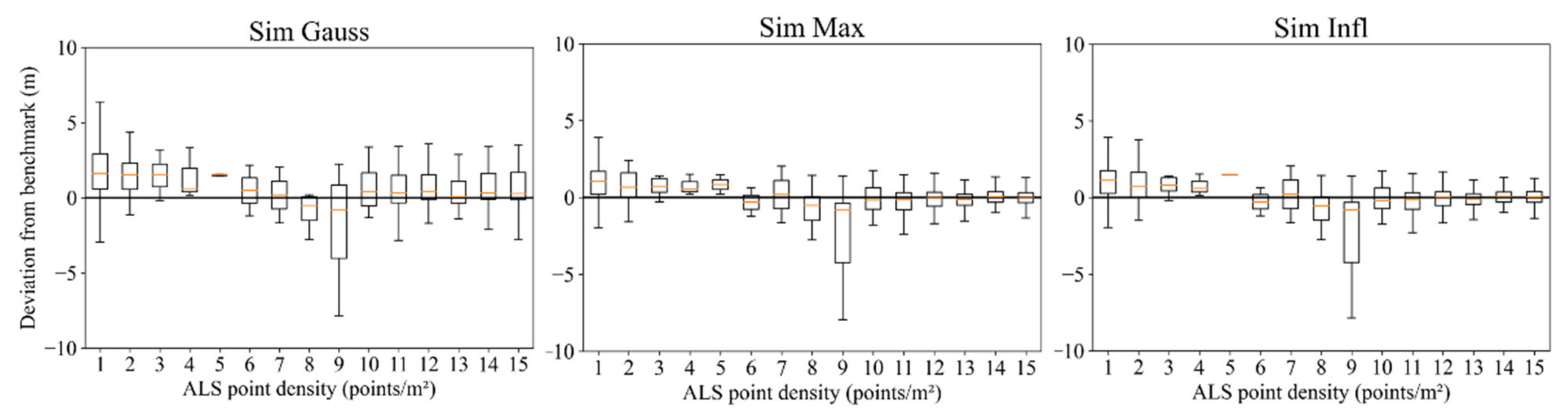
To assess the performance of the GEDI simulator’s ground detection algorithms (Gaussian, Maximum, Inflection), we compared the RH95 and RH50 metrics for different ALS point densities against the ALS benchmark.
The results for the RH95 metric (Figure 2) demonstrate that the observations simulated using the Maximum and Inflection algorithms both show smaller deviations from the benchmark values across most ALS point density categories than the Gaussian method. The interquartile ranges (IQR) of residuals produced by these two algorithms were also lower. Nevertheless, all three algorithms systematically overestimate RH95 values in lower point densities. In higher point densities (above 9 points/m2), the overestimation effect only persists for the simulator’s Gaussian algorithm. For the density range between 4 and 8 points/m2, the dataset contained few data points (n < 10, per density category); thus, no reliable conclusions could be drawn for this range.
Simulated GEDI height metrics also overestimated RH50 observations (Figure 3), particularly in lower point densities (below 2 points/m2). In higher point densities, the Maximum and Inflection methods outperformed the Gaussian algorithm markedly, although a slight systematic overestimation remained observable.
3.2. Performance of GEDI and Simulator across Forest Structural Types
In all eucalypt forest settings, simulated RH95 observations had a lower RMSE and a higher correlation with the ALS benchmark than those from the GEDI sensor (Table 4, Figure 4 and Figure 5). Furthermore, the simulator’s Maximum algorithm outperformed the Gaussian and Inflection method across all forest conditions with consistently lower RMSE and higher Pearson correlation values (Figure 4), hence why it was chosen to graphically examine the relationship between simulated and ALS benchmark heights (Figure 5).
In eucalypt forests of medium canopy height (10–30 m), both real and simulated GEDI observations were more accurate than in tall or low canopy forests (Figure 4 and Figure 5). The results also show that lower canopy cover (e.g., in the woodland category) leads to more accurate results from both GEDI and the simulator.
Real and simulated GEDI observations overestimated RH95 across all eucalypt forest types, with the simulator’s Maximum algorithm showing the smallest overestimation among all three ground detection methods. The bias using the Maximum method was frequently the closest to the bias of the GEDI instrument compared with the simulator’s other algorithms. Overall, simulated GEDI RH95 observations were more accurate (RMSE: 4.2 m, Bias: −1.3 m) than those of the actual GEDI sensor (RMSE: 9.6 m, Bias: −1.6 m).
Results for the RH50 metric were similar to those of RH95 (Table 5). When compared to the observed RMSE for the RH95 metric, one notable difference was that the RMSE of simulated GEDI RH50 observations generally were more similar to those of real GEDI. Furthermore, real GEDI observations outperformed the simulator’s Gaussian and/or Inflection algorithms across many forest types (Table 5). Pearson correlations for GEDI’s and the simulator’s RH50 metric generally were lower across all forest types in comparison with RH95.
3.3. Impact of Terrain Slope
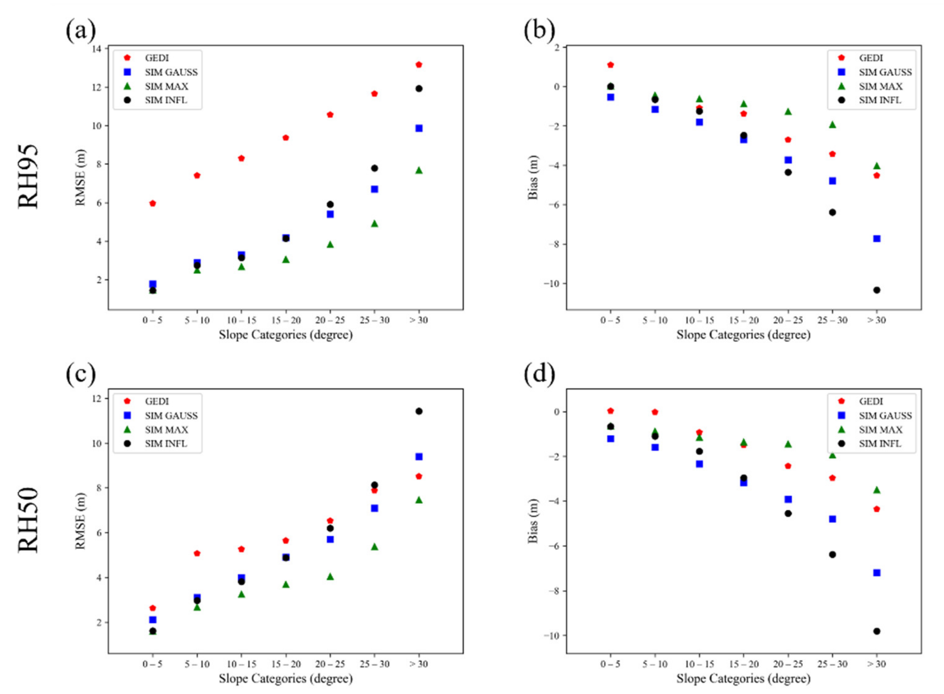
When analysing the impact of slope on real and simulated GEDI metrics, our results indicate an almost linear relationship between the RMSE of real and of simulated GEDI metrics with terrain slope, respectively. That is, the steeper the terrain, the less accurate the measurements (Figure 6).
The RMSE of real GEDI RH95 data is consistently higher than the RMSE of simulated RH95 observations (Figure 6a, Figure 7). However, for the RH50 metric on slopes larger than 30 degrees, GEDI outperformed the simulator’s Gaussian and Inflection algorithms (Figure 6c). The same two algorithms also show a greater overestimation (i.e., negative bias) of both RH95 and RH50 values than real GEDI for almost all slope categories. The Maximum algorithm not only demonstrated less overestimation but also emulated the bias of real GEDI observations the most accurately (RH95 and RH50).
For the accuracy of the ground elevation metric of real and simulated GEDI, we found that the simulator’s Maximum ground detection algorithm remained highly accurate even on slopes above 25 degrees, with biases indicating a constant slight underestimation of terrain elevation (Figure 8). Ground elevations from real GEDI observations, on the other hand, were susceptible to the effects of terrain slope, with large RMSE (>16 m) even for small slopes. We noted a slight overestimation (around 2 m) for slopes below 10 degrees, whereas medium slopes (10 to 15 degrees) produced an underestimation of a similar magnitude. The underestimation became more apparent for large slopes (25 to 30 degrees) with a bias of 10.1 m.
4. Discussion
4.1. Impact of Forest Type
Our investigation into the impact of forest type on the performance of real and simulated GEDI data showed two main trends: firstly, increased canopy cover led to a decreased performance. Secondly, real and simulated GEDI observations were more accurate in eucalypt forests of medium canopy height (10–30 m) than in low and tall eucalypt forests, as shown in Table 4 and Table 5. The bias of real and simulated RH95 observations was highest (i.e., largest overestimation) in low woodland forests, which is in agreement with the observations made for real GEDI data by Potapov et al. [24].
Generally, real GEDI RH metrics demonstrated higher RMSE and lower correlation with the benchmark compared to simulated observations. This was partly due to the absence of noise in the simulated data, as our approach did not employ the simulator’s noise function. A second cause was the geolocation uncertainty of the GEDI sensor [29], which has been determined to be 10.3 m for GEDI Version 2 data [47].
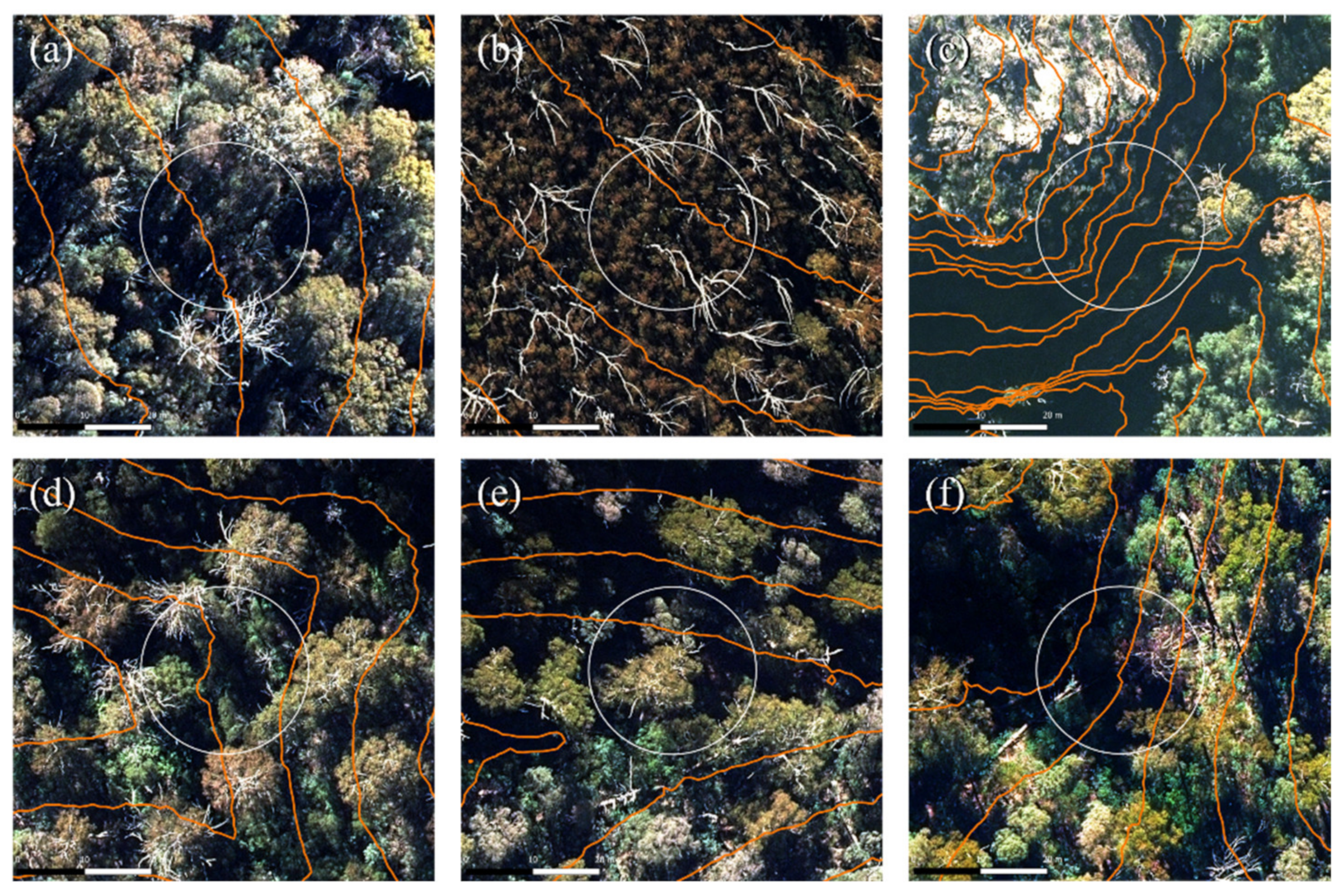
To further explore the reasons for GEDI’s underperformance compared to the simulator in the context of our study, we investigated a selection of outliers (Figure 9) with GEDI RH95 residuals larger than 20 m by comparing against high-resolution aerial imagery and terrain contour information.
One common cause for outliers was heterogenous forest structures with large gaps in the canopy, as seen in many images in Figure 9a,c,d,f. Similar observations were made by Guerra-Hernández and Pascual [29] and Roy et al. [28]. Furthermore, our investigation suggests that large dead-standing trees (Figure 9b,d) pose a challenge to GEDI’s detection of RH95, as these ”bare” objects stand out from the green canopy and thus stretch the distribution of waveform return energy representing the top of the canopy, which increases the potential magnitude of RH95 residuals. A similar effect has also been described by Hancock et al. [32] for all RH metrics where 1 minus canopy cover is close to the corresponding relative height percentile (e.g., RH75 for 25% canopy cover or RH25 for 75% canopy cover). Dead-standing trees are common in Australian eucalypt forests [48]; thus, this effect might require consideration depending on the intended application.
4.2. Impact of Slope
Large-footprint lidar sensors are prone to struggle in locations with steep terrain slope [16]. Our results show that this is not only the case for real GEDI data but can also be found in simulated GEDI observations. We found a near-linear relationship between terrain slope and RMSE, both for real and simulated RH50 and RH95 metrics, respectively. Similar observations were made for the biases, with proportionally larger RH overestimation in steeper slopes (Figure 6). These findings generally align with the results from real GEDI data in other studies [49,50]. The outliers investigated (Figure 9) also support this, as most of them were found in locations with steeper slopes. Furthermore, in our study, terrain slope had a large impact on the ground detection accuracy of real GEDI observations, with a mean underestimation of ground elevation of more than 10 m for slopes above 25 degrees, which is a finding similar to Guerra-Hernández and Pascual [29]. GEDI’s detected ground elevations serve as the reference heights to which all RH metrics are computed. Therefore, an underestimation of ground elevation leads to an overestimation of RH values. It can be expected that the observed bias in ground detection explains a portion of the RH overestimations seen in our results. Liu et al. [51], however, observed the opposite effect, using an overestimation of ground elevation to explain an underestimation of GEDI canopy height metrics. Differences in the study sites and the respective local forest types might explain these opposing results and demonstrate the need for more research into the impact of slope on GEDI observations.
4.3. Impact of ALS Point Density
Our results demonstrate that high point density ALS data facilitates more accurate RH estimates (Figure 2 and Figure 3), which is consistent with the findings from Hancock et al. [32]. Due to a lack of data from 2–9 points/m2, we could not draw reliable conclusions for that density range. However, in favourable terrain conditions (i.e., low terrain slope), our results indicate that even low point densities (<2 points/m2) lead to acceptable accuracies when applying the thresholds (absolute median bias of 1.5 m, and IQR of 3 m) set by Hancock et al. [32]. Between the simulator’s three ground detection methods, our investigation showed that the simulator’s Maximum algorithm produces more accurate RH95 and RH50 estimates than the Gaussian algorithm, both for high (>9 points/m2) and low (<2 points/m2) ALS point densities (Figure 2 and Figure 3).
The findings from this paper assist in paving the way towards using both real and simulated GEDI data in fusion approaches for structural forest monitoring, as suggested in other studies [9,27,28]. While the GEDI simulator seems well suited to complement real GEDI data by emulating bi- or multitemporal observations at the footprint level, the scarcity of historical high-density ALS point cloud datasets is a limitation. However, low-density ALS data are more readily available. Our findings suggest the preferred use of the Maximum algorithm over the Gaussian algorithm in future applications, in contrast to the approaches by Roy et al. [28] and Boucher et al. [27], as it produced the most reliable results even at lower point densities. Furthermore, its performance was superior to that of the Gaussian and Inflection algorithms across a large range of forest and terrain slope categories. In addition, observations simulated with the Maximum algorithm showed the most similar bias to real GEDI observations in most settings.
4.4. Limitations of Intercomparison
Our results indicate that the GEDI simulator compared well against the ALS benchmark data, outperforming the GEDI instrument. This was expected as both the simulated GEDI metrics and ALS benchmark metrics were derived from the same point cloud information. We acknowledge this is not an ideal approach to validation, where traditionally, independent data are preferred. However, in absence of ground truth datasets for study sites of large geographic extent, an intercomparison of real [29,50,51] or simulated [52] GEDI observations with ALS metrics is an approach that has been widely adopted.
5. Conclusions
This study assessed the performance of real and simulated GEDI observations across various sclerophyll forest types and terrain conditions by footprint-level intercomparison with an ALS-derived benchmark. The results indicate that despite the absence of noise and geolocation uncertainty in simulated data, the simulator’s Maximum algorithm provided emulated GEDI observations that have similar characteristics compared to the original. ALS point cloud data were utilised to conduct the simulations, and the results show that in level terrain conditions, even low-density ALS (<2 points/m2) is sufficient to obtain consistent results. However, in steeper slopes, both real and simulated GEDI data start to markedly overestimate canopy height, which is partly due to a decline in the ground detection accuracy. Higher canopy cover was another cause for decreased performance, while an irregular horizontal forest structure with larger gaps in the canopy proved most challenging for real GEDI data. The most accurate results were observed in medium height (10–30 m) eucalypt forests, where both GEDI and the simulator performed better than in low or tall forests.
The findings from this paper indicate the compatibility of real and simulated GEDI data for combined use in modelling approaches, paving the way towards a new facet of GEDI-aided sensor fusion methods. The GEDI instrument collects observations as a series of samples and does not directly allow for multitemporal monitoring. However, simulated observations for the same footprint locations from different points in time can be used to overcome this limitation. Such bi- or multitemporal footprint-level GEDI observations could be leveraged to improve the capturing of forest structure change over time in fusion approaches with complementary wall-to-wall remote sensing datasets such as multispectral or SAR data.
Author Contributions
Conceptualisation, S.H. (Sven Huettermann), S.J., M.S.-B. and S.H. (Samuel Hislop); methodology, S.H. (Sven Huettermann), S.J., M.S.-B. and S.H. (Samuel Hislop); software, S.H. (Sven Huettermann); validation, S.H. (Sven Huettermann); formal analysis, S.H. (Sven Huettermann); investigation, S.H. (Sven Huettermann); resources, S.H.; data curation, S.H. (Sven Huettermann); writing—original draft preparation, S.H. (Sven Huettermann); writing—review and editing, S.J., M.S.-B. and S.H. (Samuel Hislop); visualization, S.H. (Sven Huettermann); supervision, S.J., M.S.-B. and S.H. (Samuel Hislop); project administration, S.H. (Sven Huettermann); funding acquisition, S.H. (Sven Huettermann). All authors have read and agreed to the published version of the manuscript.
Funding
This research received no external funding.
Data Availability Statement
Publicly available datasets were analysed in this study. These data can be found here: https://search.earthdata.nasa.gov/search?q=gedi (accessed on 26 July 2021), and here: https://elevation.fsdf.org.au (accessed on 26 July 2021).
Acknowledgments
The authors acknowledge the support of an RMIT GOstralia Stipend Scholar scholarship from RMIT University Australia. Furthermore, the authors express their gratitude to NASA and the GEDI Mission Team, as well as Geoscience Australia and affiliated institutions, for providing the datasets that enabled this research.
Conflicts of Interest
The authors declare no conflict of interest. The funders had no role in the design of the study; in the collection, analyses, or interpretation of data; in the writing of the manuscript, or in the decision to publish the results.
References
- Slik, J.W.F.; Arroyo-Rodríguez, V.; Amarnath, G.; Griffith, D.M.; Grogan, J.; Gunatilleke, N.; Harris, D.; Harrison, R.; Hector, A.; Homeier, J.; et al. An estimate of the number of tropical tree species. Proc. Natl. Acad. Sci. USA 2015, 112, 7472–7477. [Google Scholar] [CrossRef] [PubMed] [Green Version]
- Nunes, L.; Meireles, C.; Gomes, C.; Ribeiro, N. Forest management and climate change mitigation: A review on carbon cycle flow models for the sustainability of resources. Sustainability 2019, 11, 5276. [Google Scholar] [CrossRef] [Green Version]
- Coops, N.C.; Tompalski, P.; Goodbody, T.; Queinnec, M.; Luther, J.E.; Bolton, D.K.; White, J.C.; Wulder, M.A.; van Lier, O.R.; Hermosilla, T. Modelling lidar-derived estimates of forest attributes over space and time: A review of approaches and future trends. Remote Sens. Environ. 2021, 260, 112477. [Google Scholar] [CrossRef]
- Marselis, S.M.; Abernethy, K.; Alonso, A.; Armston, J.; Baker, T.R.; Bastin, J.-F.; Bogaert, J.; Boyd, D.S.; Boeckx, P.; Burslem, D.; et al. Evaluating the potential of full-waveform lidar for mapping pan-tropical tree species richness. Glob. Ecol. Biogeogr. 2020, 29, 1799–1816. [Google Scholar] [CrossRef]
- Karna, Y.K.; Penman, T.D.; Aponte, C.; Hinko-Najera, N.; Bennett, L.T. Persistent changes in the horizontal and vertical canopy structure of fire-tolerant forests after severe fire as quantified using multi-temporal airborne lidar data. For. Ecol. Manag. 2020, 472, 118255. [Google Scholar] [CrossRef]
- Nguyen, T.; Jones, S.; Soto-Berelov, M.; Haywood, A.; Hislop, S. A Comparison of Imputation Approaches for Estimating Forest Biomass Using Landsat Time-Series and Inventory Data. Remote Sens. 2018, 10, 1825. [Google Scholar] [CrossRef] [Green Version]
- Silva, C.A.; Duncanson, L.; Hancock, S.; Neuenschwander, A.; Thomas, N.; Hofton, M.; Fatoyinbo, L.; Simard, M.; Marshak, C.Z.; Armston, J.; et al. Fusing simulated GEDI, ICESat-2 and NISAR data for regional aboveground biomass mapping. Remote Sens. Environ. 2021, 253, 112234. [Google Scholar] [CrossRef]
- Margolis, H.A.; Nelson, R.F.; Montesano, P.M.; Beaudoin, A.; Sun, G.; Andersen, H.-E.; Wulder, M.A. Combining satellite lidar, airborne lidar, and ground plots to estimate the amount and distribution of aboveground biomass in the boreal forest of North America. Can. J. For. Res. 2015, 45, 838–855. [Google Scholar] [CrossRef] [Green Version]
- Qi, W.; Saarela, S.; Armston, J.; Ståhl, G.; Dubayah, R. Forest biomass estimation over three distinct forest types using TanDEM-X InSAR data and simulated GEDI lidar data. Remote Sens. Environ. 2019, 232, 111283. [Google Scholar] [CrossRef]
- Zolkos, S.G.; Goetz, S.J.; Dubayah, R. A meta-analysis of terrestrial aboveground biomass estimation using lidar remote sensing. Remote Sens. Environ. 2013, 128, 289–298. [Google Scholar] [CrossRef]
- Kennedy, R.E.; Yang, Z.; Cohen, W.B. Detecting trends in forest disturbance and recovery using yearly Landsat time series: 1. LandTrendr—Temporal segmentation algorithms. Remote Sens. Environ. 2010, 114, 2897–2910. [Google Scholar] [CrossRef]
- White, J.C.; Saarinen, N.; Kankare, V.; Wulder, M.A.; Hermosilla, T.; Coops, N.C.; Pickell, P.D.; Holopainen, M.; Hyyppä, J.; Vastaranta, M. Confirmation of post-harvest spectral recovery from Landsat time series using measures of forest cover and height derived from airborne laser scanning data. Remote Sens. Environ. 2018, 216, 262–275. [Google Scholar] [CrossRef]
- Pascual, C.; García-Abril, A.; Cohen, W.B.; Martín-Fernández, S. Relationship between LiDAR-derived forest canopy height and Landsat images. Int. J. Remote Sens. 2010, 31, 1261–1280. [Google Scholar] [CrossRef]
- Bolton, D.; Tompalski, P.; Coops, N.; White, J.; Wulder, M.; Hermosilla, T.; Queinnec, M.; Luther, J.; Lier, O.; Fournier, R.; et al. Optimizing Landsat time series length for regional mapping of lidar-derived forest structure. Remote Sens. Environ. 2020, 239, 111645. [Google Scholar] [CrossRef]
- Sanchez-Lopez, N.; Boschetti, L.; Hudak, A.T.; Hancock, S.; Duncanson, L.I. Estimating Time Since the Last Stand-Replacing Disturbance (TSD) from Spaceborne Simulated GEDI Data: A Feasibility Study. Remote Sens. 2020, 12, 3506. [Google Scholar] [CrossRef]
- Pardini, M.; Armston, J.; Qi, W.; Lee, S.K.; Tello, M.; Cazcarra Bes, V.; Choi, C.; Papathanassiou, K.P.; Dubayah, R.O.; Fatoyinbo, L.E. Early Lessons on Combining Lidar and Multi-baseline SAR Measurements for Forest Structure Characterization. Surv. Geophys. 2019, 40, 803–837. [Google Scholar] [CrossRef]
- Duncanson, L.; Armston, J.; Disney, M.; Avitabile, V.; Barbier, N.; Calders, K.; Carter, S.; Chave, J.; Herold, M.; Crowther, T.W.; et al. The Importance of Consistent Global Forest Aboveground Biomass Product Validation. Surv. Geophys. 2019, 40, 979–999. [Google Scholar] [CrossRef] [Green Version]
- Kane, V.R.; Lutz, J.A.; Roberts, S.L.; Smith, D.F.; McGaughey, R.J.; Povak, N.A.; Brooks, M.L. Landscape-scale effects of fire severity on mixed-conifer and red fir forest structure in Yosemite National Park. For. Ecol. Manag. 2013, 287, 17–31. [Google Scholar] [CrossRef]
- Matasci, G.; Hermosilla, T.; Wulder, M.A.; White, J.C.; Coops, N.C.; Hobart, G.W.; Bolton, D.K.; Tompalski, P.; Bater, C.W. Three decades of forest structural dynamics over Canada’s forested ecosystems using Landsat time-series and lidar plots. Remote Sens. Environ. 2018, 216, 697–714. [Google Scholar] [CrossRef]
- Dubayah, R.; Blair, J.B.; Goetz, S.; Fatoyinbo, L.; Hansen, M.; Healey, S.; Hofton, M.; Hurtt, G.; Kellner, J.; Luthcke, S.; et al. The Global Ecosystem Dynamics Investigation: High-resolution laser ranging of the Earth’s forests and topography. Sci. Remote Sens. 2020, 1, 100002. [Google Scholar] [CrossRef]
- Lefsky, M.A.; Harding, D.J.; Keller, M.; Cohen, W.B.; Carabajal, C.C.; Del Bom Espirito-Santo, F.; Hunter, M.O.; de Oliveira, R. Estimates of forest canopy height and aboveground biomass using ICESat. Geophys. Res. Lett. 2005, 32, 22. [Google Scholar] [CrossRef] [Green Version]
- Scarth, P.; Armston, J.; Lucas, R.; Bunting, P. A Structural Classification of Australian Vegetation Using ICESat/GLAS, ALOS PALSAR, and Landsat Sensor Data. Remote Sens. 2019, 11, 147. [Google Scholar] [CrossRef] [Green Version]
- Healey, S.P.; Yang, Z.; Gorelick, N.; Ilyushchenko, S. Highly Local Model Calibration with a New GEDI LiDAR Asset on Google Earth Engine Reduces Landsat Forest Height Signal Saturation. Remote Sens. 2020, 12, 2840. [Google Scholar] [CrossRef]
- Potapov, P.; Li, X.; Hernandez-Serna, A.; Tyukavina, A.; Hansen, M.C.; Kommareddy, A.; Pickens, A.; Turubanova, S.; Tang, H.; Silva, C.E.; et al. Mapping global forest canopy height through integration of GEDI and Landsat data. Remote Sens. Environ. 2020, 253, 112165. [Google Scholar] [CrossRef]
- Patterson, P.L.; Healey, S.P.; Ståhl, G.; Saarela, S.; Holm, S.; Andersen, H.-E.; Dubayah, R.O.; Duncanson, L.; Hancock, S.; Armston, J.; et al. Statistical properties of hybrid estimators proposed for GEDINASA’s global ecosystem dynamics investigation. Environ. Res. Lett. 2019, 14, 65007. [Google Scholar] [CrossRef]
- Saarela, S.; Holm, S.; Healey, S.; Andersen, H.-E.; Petersson, H.; Prentius, W.; Patterson, P.; Næsset, E.; Gregoire, T.; Ståhl, G. Generalized Hierarchical Model-Based Estimation for Aboveground Biomass Assessment Using GEDI and Landsat Data. Remote Sens. 2018, 10, 1832. [Google Scholar] [CrossRef] [Green Version]
- Boucher, P.B.; Hancock, S.; Orwig, D.A.; Duncanson, L.; Armston, J.; Tang, H.; Krause, K.; Cook, B.; Paynter, I.; Li, Z.; et al. Detecting change in forest structure with simulated GEDI lidarwaveforms: A case study of the hemlock woolly adelgid (HWA; adelges tsugae) infestation. Remote Sens. 2020, 12, 1304. [Google Scholar] [CrossRef] [Green Version]
- Roy, D.P.; Kashongwe, H.B.; Armston, J. The impact of geolocation uncertainty on GEDI tropical forest canopy height estimation and change monitoring. Sci. Remote Sens. 2021, 4, 100024. [Google Scholar] [CrossRef]
- Guerra-Hernández, J.; Pascual, A. Using GEDI lidar data and airborne laser scanning to assess height growth dynamics in fast-growing species: A showcase in Spain. For. Ecosyst. 2021, 8, 14. [Google Scholar] [CrossRef]
- Tang, H.; Armston, J. Algorithm Theoretical Basis Document (ATBD) for GEDI L2BFootprint Canopy Cover and Vertical Profile Metrics. 2019. Available online: https://lpdaac.usgs.gov/documents/588/GEDI_FCCVPM_ATBD_v1.0.pdf (accessed on 20 May 2021).
- Blair, J.B.; Hofton, M.A. Modeling laser altimeter return waveforms over complex vegetation using high-resolution elevation data. Geophys. Res. Lett. 1999, 26, 2509–2512. [Google Scholar] [CrossRef]
- Hancock, S.; Armston, J.; Hofton, M.; Sun, X.; Tang, H.; Duncanson, L.I.; Kellner, J.R.; Dubayah, R. The GEDI Simulator: A Large-Footprint Waveform Lidar Simulator for Calibration and Validation of Spaceborne Missions. Earth Space Sci. 2019, 6, 294–310. [Google Scholar] [CrossRef]
- Montreal Process Implementation Group for Australia and National Forest Inventory Steering Committee. Australia’s State of the Forests Report 2018: Five-Yearly Report; Department of Agriculture, ABARES: Canberra, Australia, 2018.
- Australian Bureau of Agricultural and Resource Economics and Sciences. Forests of Australia (2018); Department of Agriculture, Water and the Environment: Canberra, Australia, 2018.
- Griebel, A.; Bennett, L.T.; Arndt, S.K. Evergreen and ever growing—Stem and canopy growth dynamics of a temperate eucalypt forest. For. Ecol. Manag. 2017, 389, 417–426. [Google Scholar] [CrossRef]
- Kennedy, R.E.; Yang, Z.; Cohen, W.B.; Pfaff, E.; Braaten, J.; Nelson, P. Spatial and temporal patterns of forest disturbance and regrowth within the area of the Northwest Forest Plan. Remote Sens. Environ. 2012, 122, 117–133. [Google Scholar] [CrossRef]
- Nguyen, T.H.; Jones, S.D.; Soto-Berelov, M.; Haywood, A.; Hislop, S. A spatial and temporal analysis of forest dynamics using Landsat time-series. Remote Sens. Environ. 2018, 217, 461–475. [Google Scholar] [CrossRef]
- Flood, N. Seasonal Composite Landsat TM/ETM+ Images Using the Medoid (a Multi-Dimensional Median). Remote Sens. 2013, 5, 6481–6500. [Google Scholar] [CrossRef] [Green Version]
- Commonwealth of Australia, G.A. Elvis—Elevation and Depth: Foundation Spatial Data. Available online: https://elevation.fsdf.org.au/ (accessed on 27 July 2021).
- McGaughey, R. FUSION/LDV; US Department of Agriculture, Forest Service, Pacific Northwest Research Station: Seattle, WA, USA, 2009.
- Victorian Government Department of Environment, Land, Water and Planning. 3D Regional Towns LiDAR. ICSM Level 2. 2020. Available online: https://elevation.fsdf.org.au/ (accessed on 26 July 2021).
- Australian Capital Territory; Aerometrex Limited. BR02096 Canberra & ACT LiDAR Tender 2020. ICSM Classification Level 3 LiDAR point cloud data (LAS 1.4). 2020. Available online: https://elevation.fsdf.org.au/ (accessed on 26 July 2021).
- Department of Finance, Services and Innovation. KOSCIUSZKO 2km × 2km Point Cloud. ICSM Classification Level 3 LiDAR point cloud data (LAS 1.2). 2017. Available online: https://elevation.fsdf.org.au/ (accessed on 26 July 2021).
- Duncanson, L.; Kellner, J.R.; Armston, J.; Dubayah, R.; Minor, D.M.; Hancock, S.; Healey, S.P.; Patterson, P.L.; Saarela, S.; Marselis, S.; et al. Aboveground biomass density models for NASA’s Global Ecosystem Dynamics Investigation (GEDI) lidar mission. Remote Sens. Environ. 2022, 270, 112845. [Google Scholar] [CrossRef]
- Qi, W.; Dubayah, R.O. Combining Tandem-X InSAR and simulated GEDI lidar observations for forest structure mapping. Remote Sens. Environ. 2016, 187, 253–266. [Google Scholar] [CrossRef]
- Jacobs Group Australia Pty Ltd. AUSIMAGE Orthophoto Product—Canberra and Queanbeyan 2017 RGB TIFF. 2017. Available online: https://elevation.fsdf.org.au/ (accessed on 26 July 2021).
- Beck, J.; Wirt, B.; Armston, J.; Hofton, M.; Luthcke, S.; Tang, H. Global Ecosystem Dynamics Investigation (GEDI) Level 02 User Guide. (Document version 2.0). 2021. Available online: https://lpdaac.usgs.gov/documents/986/GEDI02_UserGuide_V2.pdf (accessed on 22 August 2021).
- Haywood, A.; Stone, C. Estimating Large Area Forest Carbon Stocks—A Pragmatic Design Based Strategy. Forests 2017, 8, 99. [Google Scholar] [CrossRef] [Green Version]
- Fayad, I.; Baghdadi, N.; Alcarde Alvares, C.; Stape, J.L.; Bailly, J.S.; Scolforo, H.F.; Cegatta, I.R.; Zribi, M.; Le Maire, G. Terrain Slope Effect on Forest Height and Wood Volume Estimation from GEDI Data. Remote Sens. 2021, 13, 2136. [Google Scholar] [CrossRef]
- Quiros, E.; Polo, M.-E.; Fragoso-Campon, L. GEDI Elevation Accuracy Assessment: A Case Study of Southwest Spain. IEEE J. Sel. Top. Appl. Earth Obs. Remote Sens. 2021, 14, 5285–5299. [Google Scholar] [CrossRef]
- Liu, A.; Cheng, X.; Chen, Z. Performance evaluation of GEDI and ICESat-2 laser altimeter data for terrain and canopy height retrievals. Remote Sens. Environ. 2021, 264, 112571. [Google Scholar] [CrossRef]
- Schneider, F.D.; Ferraz, A.; Hancock, S.; Duncanson, L.I.; Dubayah, R.O.; Pavlick, R.P.; Schimel, D.S. Towards mapping the diversity of canopy structure from space with GEDI. Environ. Res. Lett. 2020, 15, 115006. [Google Scholar] [CrossRef]
Figure 1.
The four study sites (red) with selected Global Ecosystem Dynamics Investigation (GEDI) footprints (black) across the Australia states Victoria, New South Wales, and Australian Capital Territory.
Figure 1.
The four study sites (red) with selected Global Ecosystem Dynamics Investigation (GEDI) footprints (black) across the Australia states Victoria, New South Wales, and Australian Capital Territory.

Figure 2.
Deviation from true RH95 for the simulator’s Gaussian algorithm (left), Maximum algorithm (centre), and Inflection algorithm (right). Only observations with a terrain slope below 5 degrees were considered for this figure. Note that the density categories between 3 and 9 points/m2 have low (<30) numbers of samples. Positive values indicate an overestimation of RH95.

Figure 3.
Deviation from true RH50 for the simulator’s Gaussian algorithm (left), Maximum algorithm (centre), and Inflection algorithm (right). Only observations with a terrain slope below 5 degrees were considered for this figure. Note that the density categories between 3 and 9 points/m2 have low (<30) numbers of samples. Positive values indicate an overestimation of RH50.

Figure 4.
RH95 from GEDI compared to ALS benchmark heights, for eucalypt forests with canopy height/cover: (a) Medium/Open, (b) Tall/Open, (c) Low/Woodland, (d) Medium/Woodland, (e) Tall/Woodland.
Figure 4.
RH95 from GEDI compared to ALS benchmark heights, for eucalypt forests with canopy height/cover: (a) Medium/Open, (b) Tall/Open, (c) Low/Woodland, (d) Medium/Woodland, (e) Tall/Woodland.

Figure 5.
RH95 from the simulator’s Maximum algorithm compared to ALS benchmark heights, for eucalypt forests with canopy height/cover: (a) Medium/Open, (b) Tall/Open, (c) Low/Woodland, (d) Medium/Woodland, (e) Tall/Woodland.
Figure 5.
RH95 from the simulator’s Maximum algorithm compared to ALS benchmark heights, for eucalypt forests with canopy height/cover: (a) Medium/Open, (b) Tall/Open, (c) Low/Woodland, (d) Medium/Woodland, (e) Tall/Woodland.

Figure 6.
Impact of the terrain slope on RMSE (a,c) and bias (b,d) for real GEDI observations (red) and simulated GEDI observations of RH95 (a,b) and RH50 (c,d) using the Gaussian (blue), Maximum (green) and Inflection algorithm (black).
Figure 6.
Impact of the terrain slope on RMSE (a,c) and bias (b,d) for real GEDI observations (red) and simulated GEDI observations of RH95 (a,b) and RH50 (c,d) using the Gaussian (blue), Maximum (green) and Inflection algorithm (black).

Figure 7.
Intercomparison of GEDI (left column), Gaussian simulator (centre column), and Maximum simulator (right column) with the RH95 benchmark values, for terrain slopes of 0–5 degrees (bottom row), 15–20 degrees (centre row), and >30 degrees (top row).
Figure 7.
Intercomparison of GEDI (left column), Gaussian simulator (centre column), and Maximum simulator (right column) with the RH95 benchmark values, for terrain slopes of 0–5 degrees (bottom row), 15–20 degrees (centre row), and >30 degrees (top row).

Figure 8.
Ground elevation residuals for simulated (Maximum algorithm, blue) and real (orange) GEDI observations. A positive difference indicates an overestimation.
Figure 8.
Ground elevation residuals for simulated (Maximum algorithm, blue) and real (orange) GEDI observations. A positive difference indicates an overestimation.

Figure 9.
Six example outliers with a large deviation of GEDI RH95 from true RH95. These were randomly selected from all observations from the Canberra site that deviated more than 20 m from the benchmark value. The GEDI footprint is represented by a white circle, the orange lines represent terrain contours in 5 m vertical intervals. (a,b) show examples of dead-standing trees, whereas in (c–f) steep slopes and gaps in the canopy are likely reasons for large RH95 residuals. High resolution aerial photography (0.1 m) shown to aid investigation, reprinted with permission from Jacobs Group Australia Pty Ltd [46].


Table 1.
Number of footprints per forest type.
| Forest Type | Total Footprints |
|---|---|
| Casuarina | 16 |
| Eucalypt Mallee Open | 28 |
| Eucalypt Mallee Woodland | 158 |
| Eucalypt Low Woodland | 1914 |
| Eucalypt Medium Closed | 29 |
| Eucalypt Medium Open | 7759 |
| Eucalypt Medium Woodland | 1215 |
| Eucalypt Tall Closed | 4 |
| Eucalypt Tall Open | 3024 |
| Eucalypt Tall Woodland | 164 |
| Rainforest | 12 |
| Softwood plantation | 671 |
| Other native forest | 371 |
| Unallocated | 251 |
Table 2.
Number of footprints per terrain slope category.
| Slope Category (Degree) | Total Footprints |
|---|---|
| 0–5 | 3479 |
| 5–10 | 2010 |
| 10–15 | 1884 |
| 15–20 | 1919 |
| 20–25 | 1882 |
| 25–30 | 1798 |
| >30 | 2644 |
Table 3.
Technical specifics of the airborne laser scanning (ALS) data sets from the four study sites.
Table 3.
Technical specifics of the airborne laser scanning (ALS) data sets from the four study sites.
| Site Name | Scanner | Average Point Density (Points/m2) | Year | Horizontal/Vertical Accuracy | Number of Footprints | ALS Data Source |
|---|---|---|---|---|---|---|
| Bendigo | Trimble AX60 | 22 * | 2020 | 0.3 m/0.1 m | 2582 | [41] |
| Bright | Trimble AX60 | 22 * | 2020 | 0.3 m/0.1 m | 1203 | [41] |
| Canberra | Riegl VQ780i | 23 | 2020 | 0.3 m/0.1 m | 3191 | [42] |
| Kosciuszko | Leica ALS50 | 0.4 | 2017 | 0.8 m/0.3 m (95% confidence) | 8640 | [43] |
* Values have been manually determined from the dataset, as accurate metadata was unavailable.
Table 4.
RMSE, Pearson correlation r, and bias of real and simulated (Sim) GEDI data (RH95) in different eucalypt forest types.
Table 4.
RMSE, Pearson correlation r, and bias of real and simulated (Sim) GEDI data (RH95) in different eucalypt forest types.
| Eucalypt Low Woodland | Eucalypt Medium Woodland | Eucalypt Medium Open | Eucalypt Tall Woodland | Eucalypt Tall Open | ||
|---|---|---|---|---|---|---|
| RMSE (m) | GEDI | 9.47 | 5.19 | 8.46 | 8.64 | 14.03 |
| Sim Gauss | 5.39 | 2.84 | 5.44 | 5.47 | 7.23 | |
| Sim Max | 3.34 | 1.58 | 4.27 | 3.28 | 5.80 | |
| Sim Infl | 6.23 | 2.75 | 6.22 | 5.44 | 8.46 | |
| r | GEDI | 0.45 | 0.55 | 0.54 | 0.29 | 0.42 |
| Sim Gauss | 0.88 | 0.93 | 0.87 | 0.77 | 0.91 | |
| Sim Max | 0.91 | 0.97 | 0.88 | 0.89 | 0.92 | |
| Sim Infl | 0.84 | 0.92 | 0.85 | 0.78 | 0.89 | |
| Bias (m) | GEDI | −4.54 | −0.55 | −1.36 | −0.46 | −1.60 |
| Sim Gauss | −4.13 | −1.93 | −2.97 | −2.19 | −4.28 | |
| Sim Max | −1.76 | −0.70 | −1.26 | −0.50 | −1.76 | |
| Sim Infl | −4.58 | −1.54 | −3.32 | −2.63 | −5.51 |
Table 5.
RMSE, Pearson correlation r, and bias of real and simulated (Sim) GEDI data (RH50) in different eucalypt forest types.
Table 5.
RMSE, Pearson correlation r, and bias of real and simulated (Sim) GEDI data (RH50) in different eucalypt forest types.
| Eucalypt Low Woodland | Eucalypt Medium Woodland | Eucalypt Medium Open | Eucalypt Tall Woodland | Eucalypt Tall Open | ||
|---|---|---|---|---|---|---|
| RMSE (m) | GEDI | 5.12 | 2.83 | 5.78 | 4.27 | 8.20 |
| Sim Gauss | 4.75 | 2.74 | 5.75 | 4.84 | 7.54 | |
| Sim Max | 2.93 | 1.45 | 4.61 | 3.20 | 5.94 | |
| Sim Infl | 5.57 | 2.57 | 6.42 | 4.76 | 8.75 | |
| r | GEDI | 0.28 | 0.18 | 0.36 | 0.25 | 0.14 |
| Sim Gauss | 0.62 | 0.70 | 0.72 | 0.38 | 0.71 | |
| Sim Max | 0.67 | 0.83 | 0.72 | 0.41 | 0.72 | |
| Sim Infl | 0.57 | 0.68 | 0.70 | 0.40 | 0.67 | |
| Bias (m) | GEDI | −2.77 | −0.70 | −1.60 | −1.15 | −3.25 |
| Sim Gauss | −3.51 | −2.02 | −3.48 | −2.06 | −4.95 | |
| Sim Max | −1.14 | −0.78 | −1.77 | −0.37 | −2.43 | |
| Sim Infl | −3.96 | −1.63 | −3.83 | −2.50 | −6.18 |
Publisher’s Note: MDPI stays neutral with regard to jurisdictional claims in published maps and institutional affiliations. |
© 2022 by the authors. Licensee MDPI, Basel, Switzerland. This article is an open access article distributed under the terms and conditions of the Creative Commons Attribution (CC BY) license (https://creativecommons.org/licenses/by/4.0/).
Share and Cite
MDPI and ACS Style
Huettermann, S.; Jones, S.; Soto-Berelov, M.; Hislop, S. Intercomparison of Real and Simulated GEDI Observations across Sclerophyll Forests. Remote Sens. 2022, 14, 2096. https://0-doi-org.brum.beds.ac.uk/10.3390/rs14092096
AMA Style
Huettermann S, Jones S, Soto-Berelov M, Hislop S. Intercomparison of Real and Simulated GEDI Observations across Sclerophyll Forests. Remote Sensing. 2022; 14(9):2096. https://0-doi-org.brum.beds.ac.uk/10.3390/rs14092096
Chicago/Turabian StyleHuettermann, Sven, Simon Jones, Mariela Soto-Berelov, and Samuel Hislop. 2022. "Intercomparison of Real and Simulated GEDI Observations across Sclerophyll Forests" Remote Sensing 14, no. 9: 2096. https://0-doi-org.brum.beds.ac.uk/10.3390/rs14092096
Note that from the first issue of 2016, this journal uses article numbers instead of page numbers. See further details here.