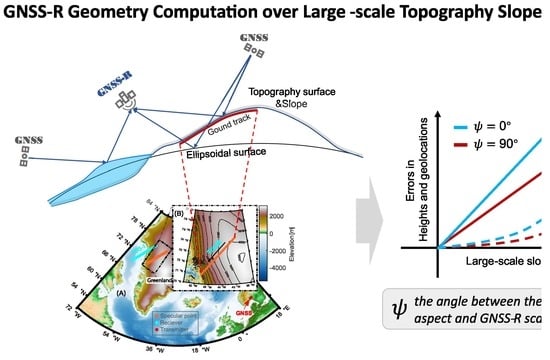
A New Empirical Model for Initialization
A fast and accurate initial input can expedite the estimation of precise specular points. Previous analyses are commonly based on the subpoint of the receiver on the Earth’s surface or the weighted distance along the vector from the receiver to the transmitter and then scaled down to the Earth’s surface to get the initial specular point [
30,
38], as shown in
Figure A1. We can find an estimated point
on
, and then set the subpoint,
, of
on the sphere Earth’s surface as the initial estimation of specular point. The precision of estimation obtained from this method depends on the position of
. In previous studies,
is determined approximately by the weighted distance approach, and its expression reads:
where
is the radius of the Earth sphere,
is the weight and calculated by:
where
and
are the subpoints of the receiver and transmitter in
Figure A1. However, unaccepted large errors can be found in low elevation angle situations based on these approaches, which is caused by the incorrect hypothesis that the heights of the receiver and transmitter to the tangent plane at the specular point are equal to the ellipsoid height. Therefore, if the heights of the receiver and transmitter to the tangent plane at the specular point are known and the Earth is assumed spherical, this method is theoretically valid and reliable. In this work, we proposed an empirical method to determine the accuracy point
.
Figure A1.
The geometry of initial specular points estimation. is the specular point; and denote the receiver and transmitter; and are the orthographic points on the tangent plane to the sphere Earth at ; is the intersection of vector and .
Figure A1.
The geometry of initial specular points estimation. is the specular point; and denote the receiver and transmitter; and are the orthographic points on the tangent plane to the sphere Earth at ; is the intersection of vector and .
In
Figure A1, once the vertical distances of
and
to the tangent plane are known, the intersection point
of the vector
and the vector
can be obtained by (A2) with a new weight calculated by:
Then the initial specular point can be estimated by scaling the
to the sphere Earth surface based on Equation (A1). In this study, the radius of the sphere Earth
is set to the mean radius of WGS-84 ellipsoid (6378 km). After obtaining the position of
in
Figure A1, we can simply transform it to the WGS84 ellipsoid surface by multiplying the transformation matrix according to the method in [
25] to reduce the errors caused by the Earth’s curvature, as follows:
where
and
are the semi-major axis and semi-minor axis, respectively.
However, it is impossible to get this precise ratio
only based on the position of the receiver and transmitter. Therefore, we try to estimate it empirically. Firstly, we implement a comprehensive simulation corresponding to different orbit heights from 300 km to 1200 km. In each simulation, the geocentric angle
, shown in
Figure A1, between receiver and transmitter is calculated to figure out the relationship between
and ratio
. Here an example corresponding to the orbit height of 500 km is shown in
Figure A2.
Figure A2.
The relationship between geocentric angles and distance ratio . In this simulation, 100,000 events were involved, and a histogram plot of the elevation angle is shown in the top right corner.
Figure A2.
The relationship between geocentric angles and distance ratio . In this simulation, 100,000 events were involved, and a histogram plot of the elevation angle is shown in the top right corner.
In
Figure A2, simulations are obtained in the situation where the receiver height is 500 km and the transmitter height is 20,200 km (GPS), with an even distribution in the elevation angles. It can be found that the true ratio
demonstrates a smooth and regular trend along with the cosine value of the geocentric angle
. Thus, here a cubic-polynomial fitting method is applied to fit the dot trend and it exhibits a decent performance. The fitting model is as follows:
where
are the coefficients of the fitting model.
Once the curve corresponding to different orbit heights is fitted, the relatively precise ratio
can be estimated by inputting the geocentric angle
, which is easy to calculate. According to this idea, a comprehensive simulation related to different orbit heights and geocentric angles is implemented. Based on the simulations, it finds that the coefficients along the varied orbit heights of the receiver demonstrate regular and smooth changes, as the dot presented in
Figure A3.
Figure A3.
Variations of coefficients in Equation (A7) versus the orbital heights of the receiver. The results are obtained by the 100,000 simulations at each orbit height situation.
Figure A3.
Variations of coefficients in Equation (A7) versus the orbital heights of the receiver. The results are obtained by the 100,000 simulations at each orbit height situation.
In
Figure A3, the variations of coefficients in Equation (A7) along the increasing orbit heights show a monotonous trend of change. To reduce the computational overhead, a cubic-polynomial fitting method is employed to estimate the coefficients with respect to different orbit heights of receivers. The fitted model is as follows, and fitting results are given in
Figure A3:
where
are the coefficients of the fitting model, which are used to estimate the coefficients
in Equation (A7). Further tests reveal that the cubic-polynomial curve is not the best fit, but it is decent for the initial estimation and minimizing calculation load. The coefficients from the fits along the orbit heights are given in
Table A1. To ensure the order of magnitude of the coefficient, the unit of
is 1000 km.
Table A1.
Parameter fitting results of coefficients in Equation (A8) for empirical model functions.
Table A1.
Parameter fitting results of coefficients in Equation (A8) for empirical model functions.
| | | | |
|---|
| 0.04478 | −0.1325 | 0.1333 | −0.04484 |
| −0.08442 | 0.2599 | −0.2892 | 0.1341 |
| 0.03152 | −0.09935 | 0.1240 | −0.1332 |
| 0.008292 | −0.03064 | 0.08151 | 0.04403 |
Combining Equations (A1)–(A8),
Table A1, and the transformed method in [
25], the initial specular point can be estimated rapidly. However, we should be aware that the ratio
will also be affected by different heights of the transmitter. A height of 20,200 km is fixed in the simulation, which is slightly different from the natural orbits of GPS satellites. So, the position of the transmitter should be scaled to the fixed height before the initial estimation to weaken the relatively small orbital height influence, as follows:
where
is the transmitter position,
is the mean orbital height of the transmitter, 20,200 km for GPS satellites.
is the mean Earth’s radius (6378 km). Then,
is entered in Equation (A2).
To verify this empirical method, another simulation covering the orbit height from 300 km to 1200 km was carried out, and its statistics of tridimensional errors (Euclidean distance) are presented in
Figure A4.
Figure A4.
Statistics of empirical specular point estimation errors corresponding to different orbit height situations. The radius of the Earth sphere is 6378 km, and the fixed height of the transmitter is 20,200 km. A quantity of 900,000 and 320,000 events (only GPS) from the TDS-1(cross dots) and CYGNSS (circular dots) satellites are also used to validate this empirical model, respectively.
In
Figure A4, the mean, median, and standard deviation (STD) of tridimensional errors are calculated. Overall, the standard deviation is almost maintained below 1.5 km, and mean and median errors are almost less than 3 km through all orbit height situations. Results from the CYGNSS and TDS-1 satellites validate this method and their error statistics are close to the simulations when the GPS satellite is the transmitter, which turns out that the empirical model can implement a fast and precise initial geometry calculation. Similarly, the coefficients of the fitting model (Equation (A8)) for Glonass, Galileo, and Beidou (MEO) systems are given in the following tables.
Table A2.
Coefficients of the fitting model for Glonass system (Mean orbital height: 19,000 km).
Table A2.
Coefficients of the fitting model for Glonass system (Mean orbital height: 19,000 km).
| | | | |
|---|
| 0.0695 | −0.1987 | 0.1874 | −0.05558 |
| −0.1316 | 0.387 | −0.3958 | 0.1581 |
| 0.05733 | −0.1688 | 0.1838 | −0.1515 |
| 0.005163 | −0.02294 | 0.07767 | 0.049 |
Table A3.
Coefficients of the fitting model for Galileo system (Mean orbital height: 23,220 km).
Table A3.
Coefficients of the fitting model for Galileo system (Mean orbital height: 23,220 km).
| | | | |
|---|
| 0.05364 | −0.1556 | 0.1507 | −0.04809 |
| −0.09738 | 0.2902 | −0.3043 | 0.1306 |
| 0.03784 | −0.1125 | 0.125 | −0.1199 |
| 0.006253 | −0.02476 | 0.07224 | 0.03729 |
Table A4.
Coefficients of the fitting model for Beidou system (Mean orbital height (MEO): 21,550 km).
Table A4.
Coefficients of the fitting model for Beidou system (Mean orbital height (MEO): 21,550 km).
| | | | |
|---|
| 0.05879 | −0.1698 | 0.1631 | −0.05077 |
| −0.1085 | 0.322 | −0.335 | 0.1403 |
| 0.04405 | −0.1306 | 0.1443 | −0.1308 |
| 0.005997 | −0.02447 | 0.07456 | 0.04127 |
For different orbital height systems, dedicated coefficients for Glonass, Galileo, and Beidou (MEO) systems can achieve a similar precision (within 1.5 km) as the GPS system shown in
Figure A4 in the fastest way.


 ,
, 


