
Using Optical Water-Type Classification in Data-Poor Water Quality Assessment: A Case Study in the Torres Strait †


Abstract
:1. Introduction
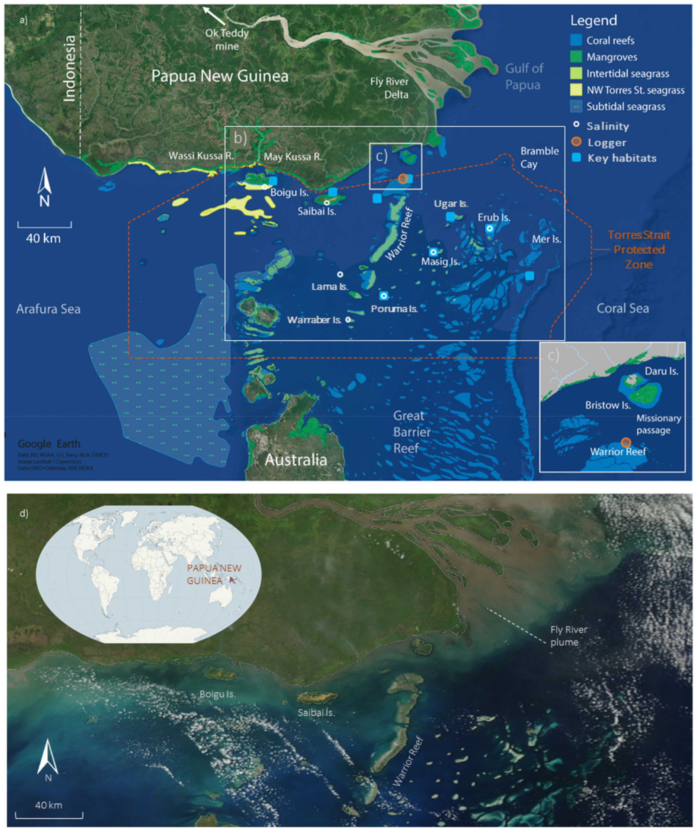
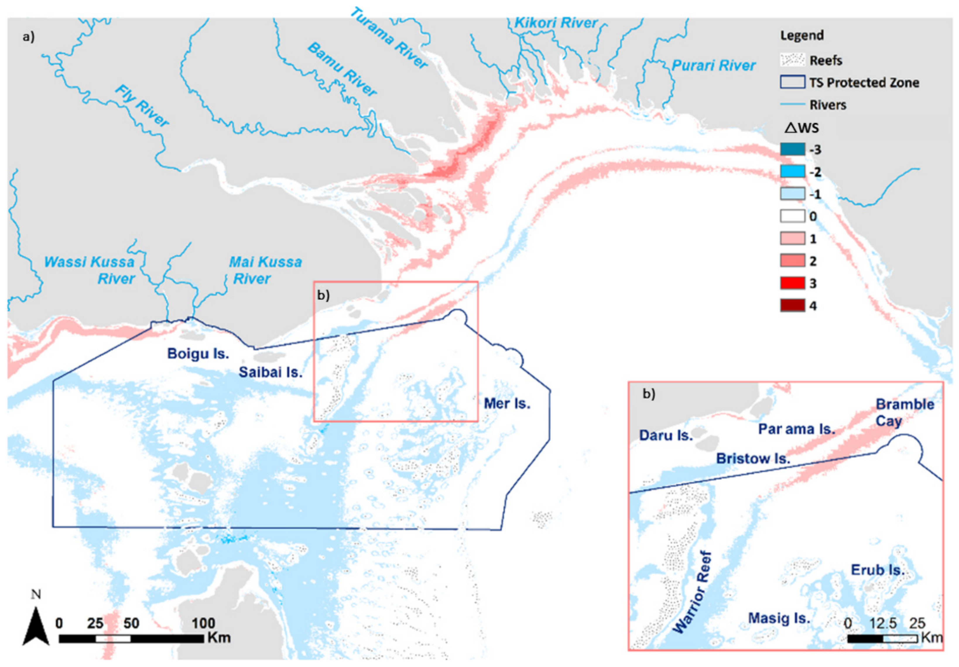
2. Study Area
3. Materials and Method
3.1. Satellite Data
3.2. Water Quality Monitoring
- (a)
- SSC measurements
- (b)
- Optical dataset
- (c)
- Salinity data
- (d)
- Continuous logger data
3.3. Data Analyses
3.3.1. Spatial Analyses
3.3.2. Statistical Analyses
3.3.3. Qualitative Assessment
4. Results
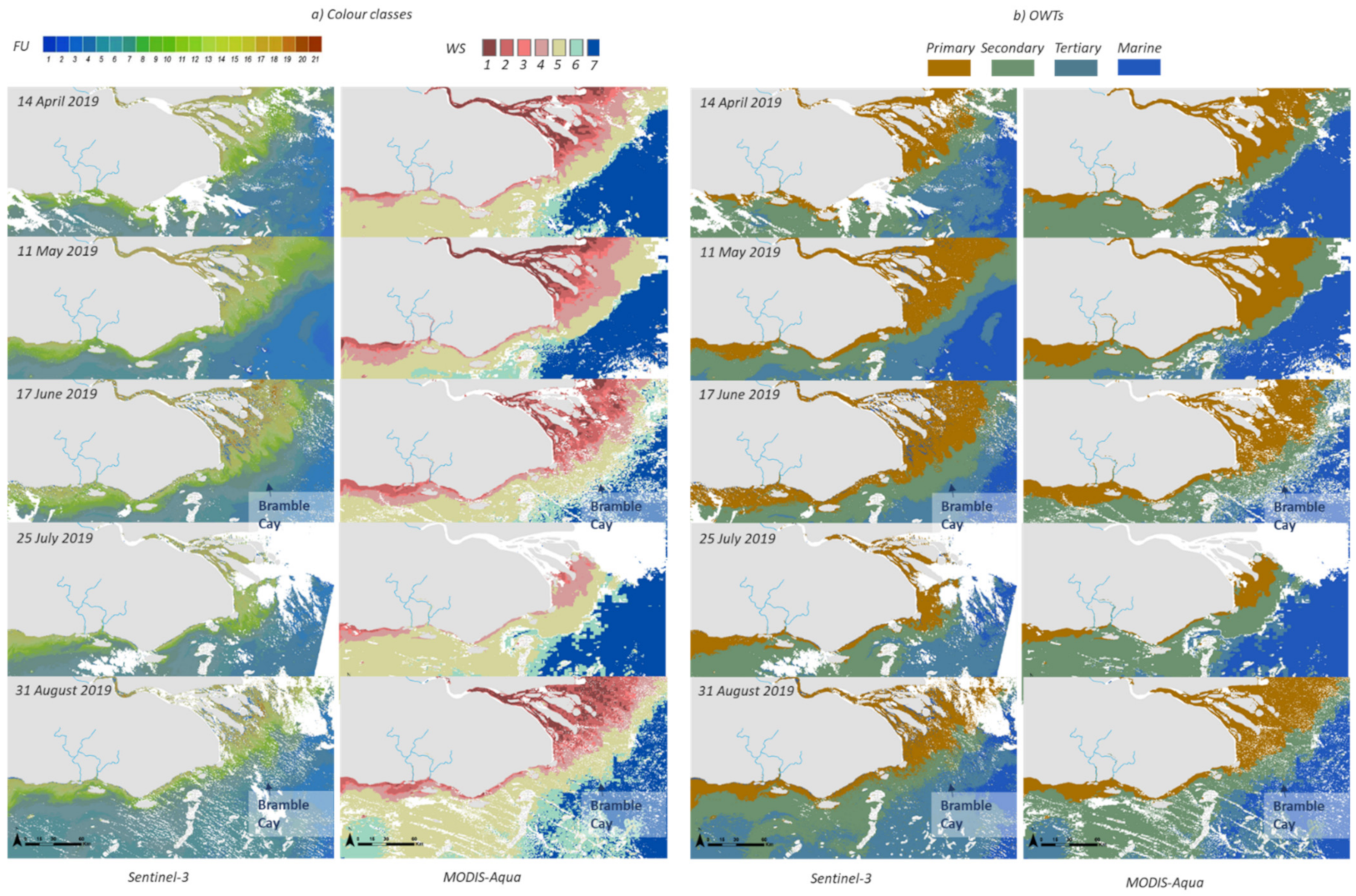
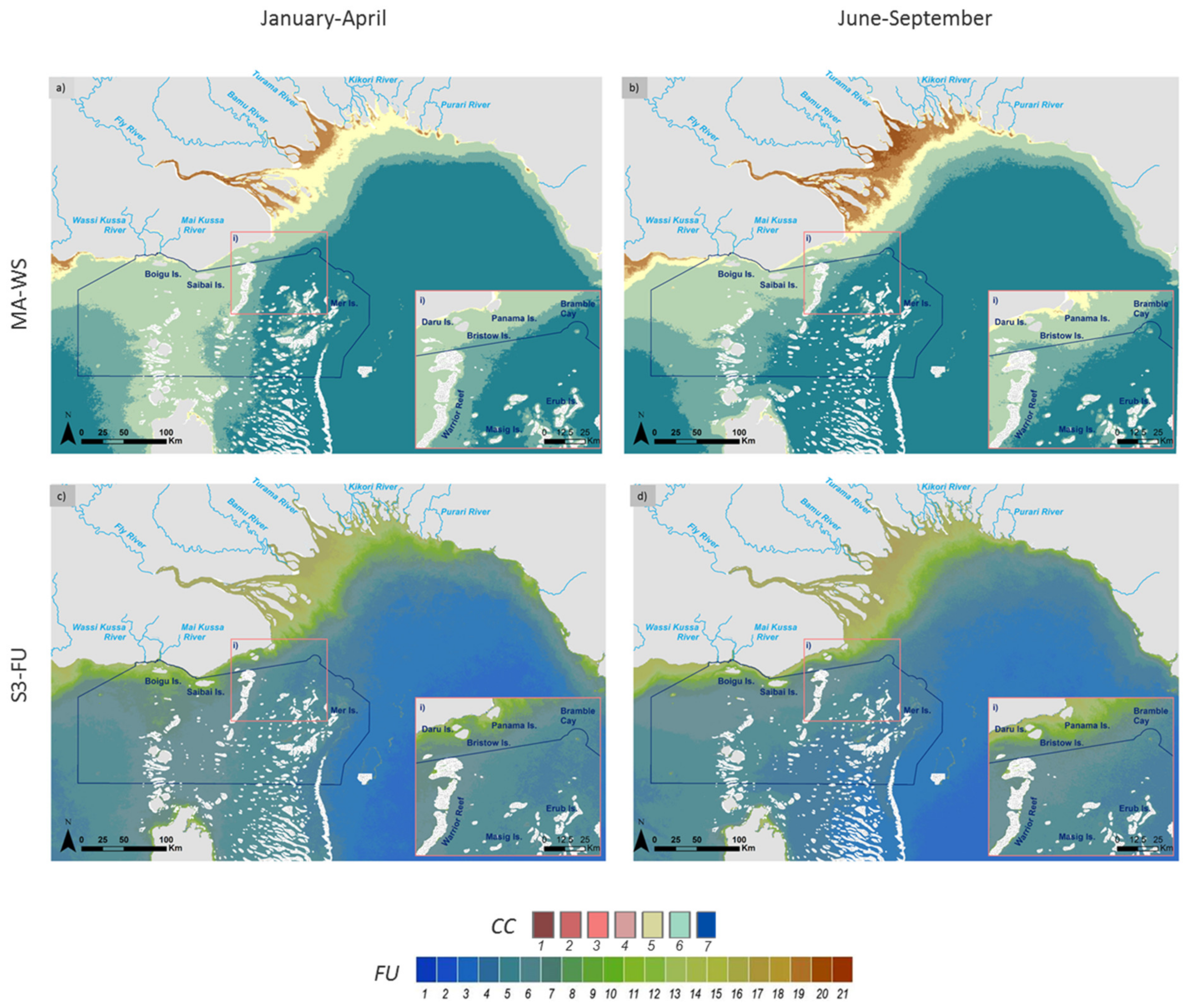
4.1. MODIS Water Type Maps
4.1.1. Verification
4.1.2. Composition
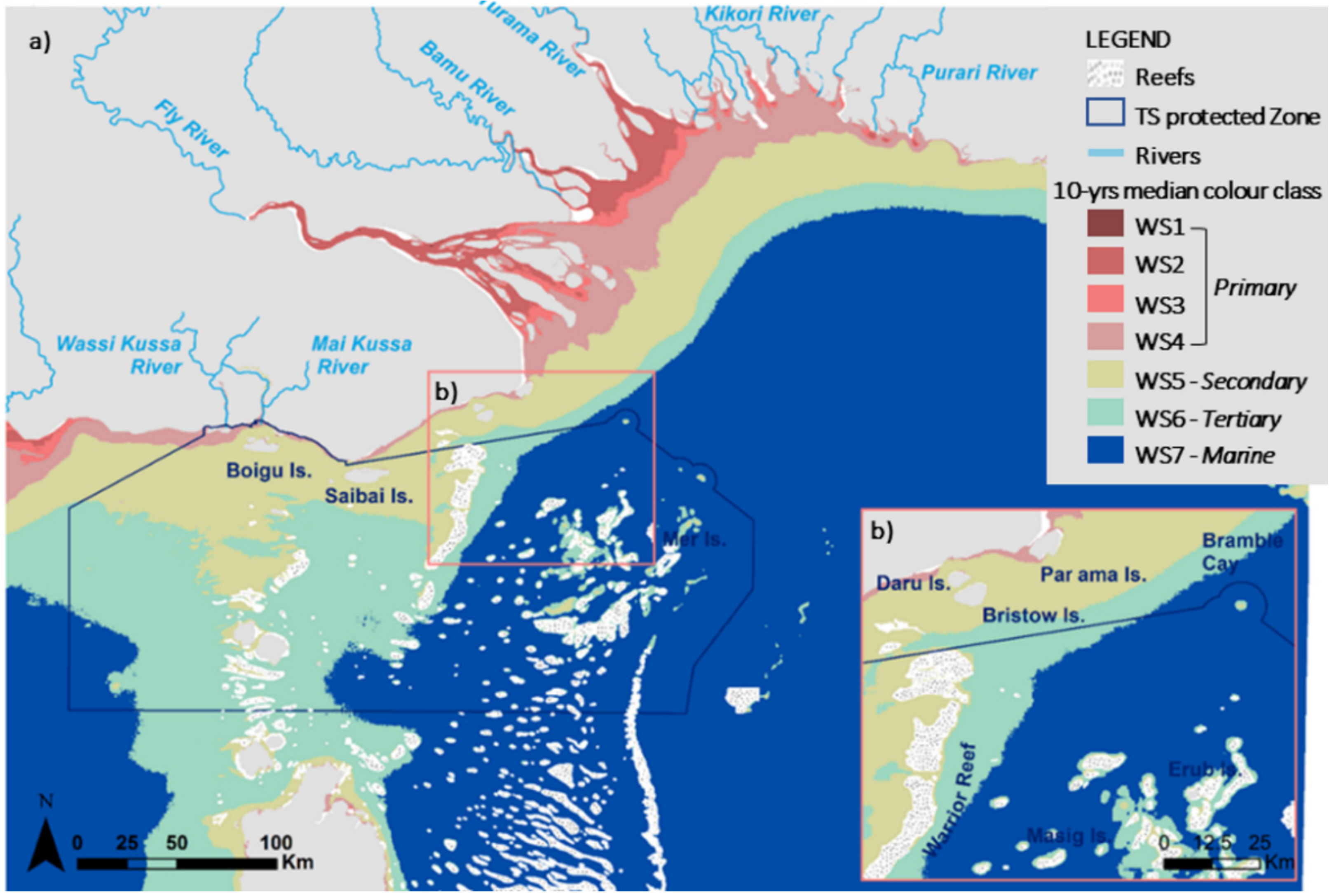
4.1.3. Decadal Colour Patterns
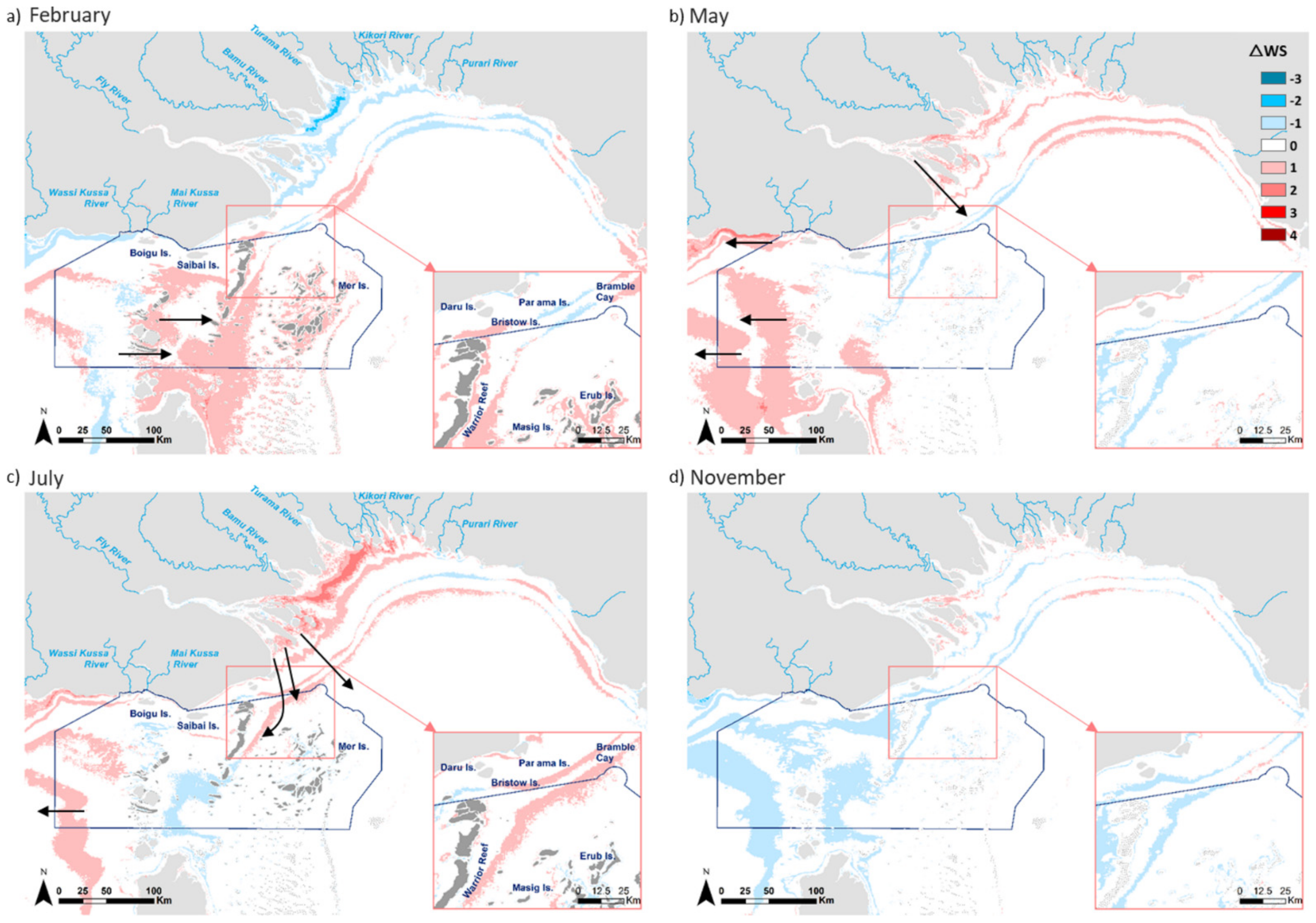
4.2. Seasonal Patterns
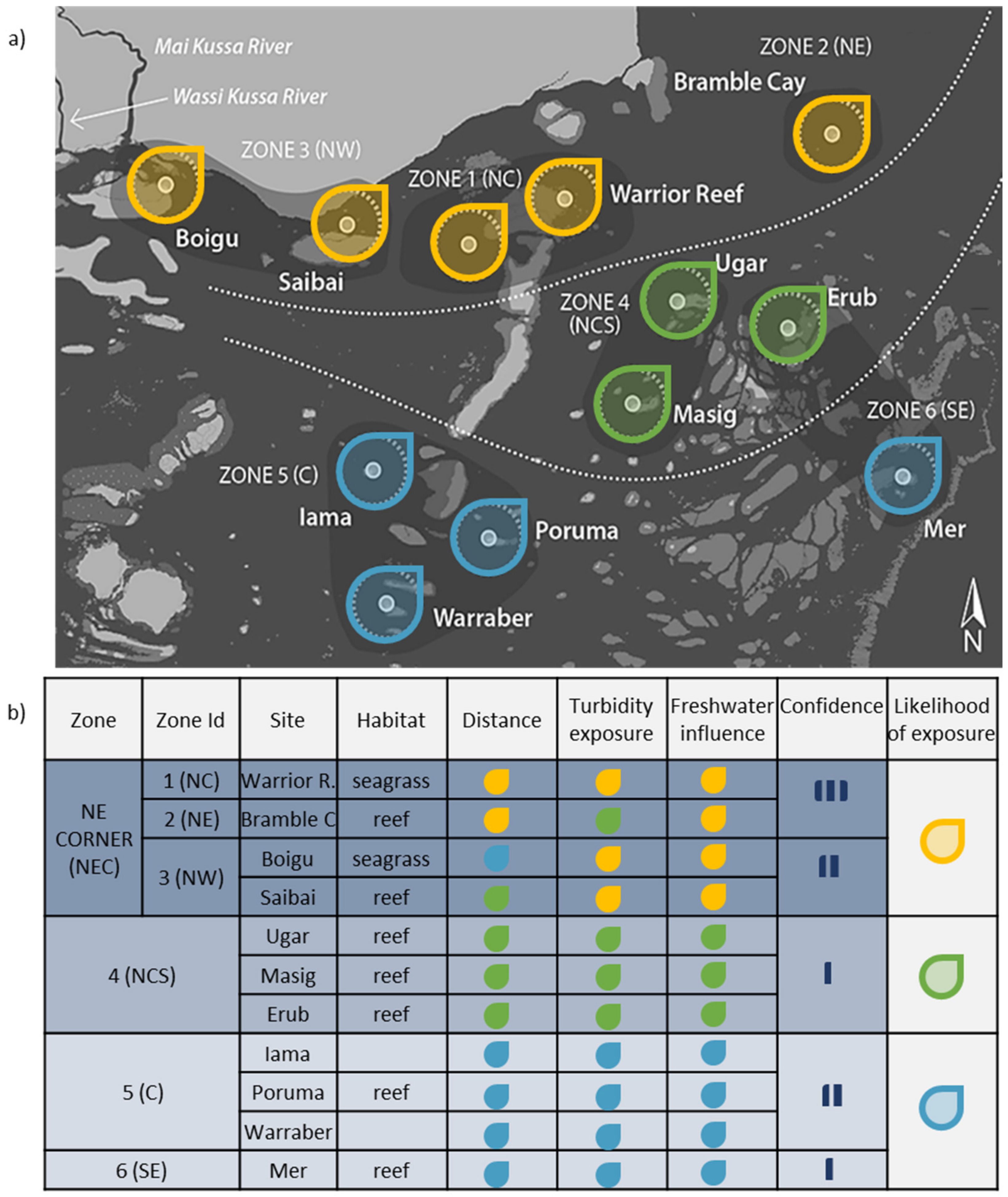
4.3. Ecosystem Exposure to Turbid Waters
4.4. Freshwater Intrusions
4.5. Qualitative Assessment
5. Discussion
6. Conclusions
Author Contributions
Funding
Institutional Review Board Statement
Informed Consent Statement
Data Availability Statement
Acknowledgments
Conflicts of Interest
Abbreviations
| Regions | |
| GBR | Great Barrier Reef Marine Park |
| PNG | Papua New Guinea |
| TS | Torres Strait |
| Satellites | |
| MA | MODIS-Aqua satellite |
| S3 or S2 | Sentinel-3 or 2 satellites |
| Colour classification scales | |
| FU | Forel-Ule colour scale |
| WS | Wet Season colour scale |
| OWT | Optical Water types |
| Water quality parameters | |
| SSC | Suspended sediment concentrations |
| CDOM | coloured dissolved organic matters |
| Chl-a | chlorophyll-a |
| SDD | Secchi Disk Depth |
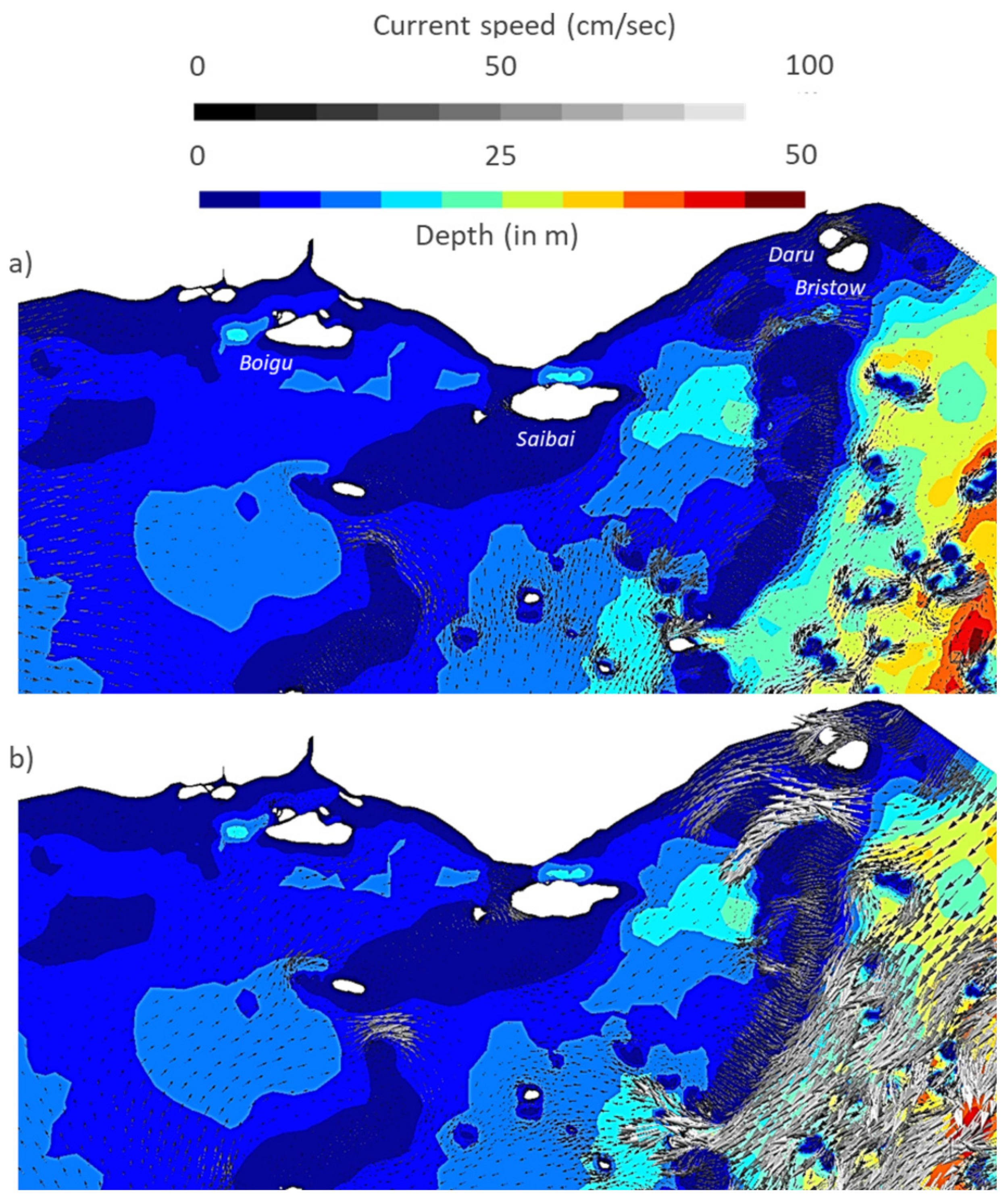
Appendix A. SLIM Model Outputs

Appendix B. Field Data
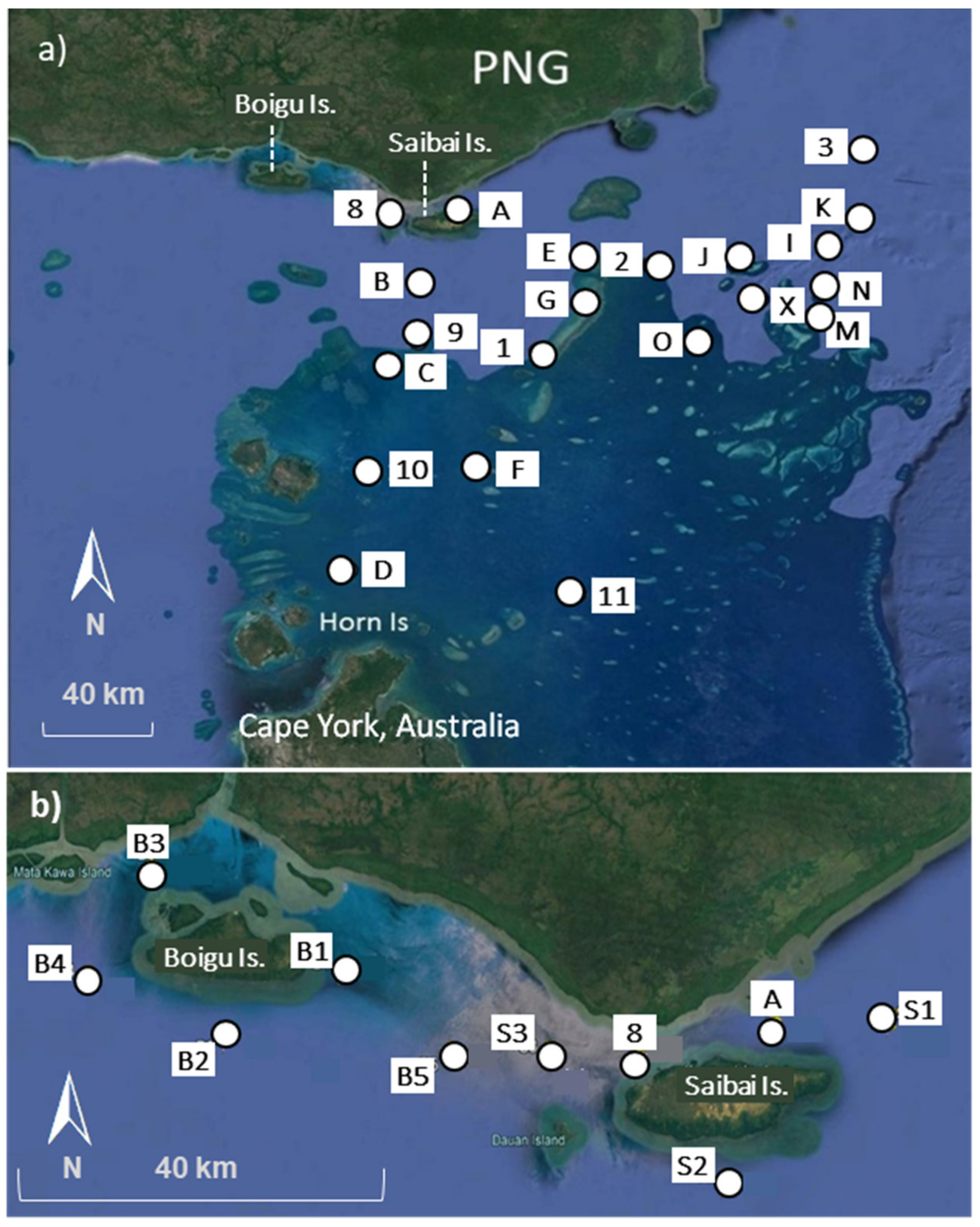
Appendix B.1. SSC Measurements


| Sample ID | Date | SSC | Turbidity | MA-WS |
|---|---|---|---|---|
| Loc 1 | 3/10/2016 | 1.7 | 0.8 | na |
| Loc G | 3/10/2016 | 1.9 | 1.3 | na |
| Loc 2 | 4/10/2016 | 2.5 | 0.6 | 7.0 |
| Loc J | 4/10/2016 | 2.3 | 0.4 | na |
| Loc 3 | 5/10/2016 | 0.7 | 0.3 | 5.0 |
| Loc K | 5/10/2016 | 5.0 | 0.6 | 6.0 |
| Loc I | 5/10/2016 | 1.6 | 0.4 | 5.0 |
| Loc M | 6/10/2016 | 0.8 | 0.8 | 6.0 |
| Erub | 6/10/2016 | 1.1 | 0.6 | 5.0 |
| Erub (duplicate) | 6/10/2016 | 1.0 | 0.5 | 5.0 |
| Loc X | 7/10/2016 | 3.5 | 0.9 | na |
| Masig | 8/10/2016 | 0.6 | 0.4 | na |
| Masig 2 | 8/10/2016 | 0.8 | 0.4 | na |
| Site E | 10/10/2016 | 7.3 | 2.7 | na |
| Site 8 | 11/10/2016 | 12.0 | 8.8 | na |
| Site A | 11/10/2016 | 11.2 | 8.0 | 5.0 |
| Site A (duplicate) | 11/10/2016 | 10.4 | 8.0 | 5.0 |
| Site B | 12/10/2016 | 4.8 | 2.1 | 6.0 |
| Site 9 | 13/10/2016 | 3.0 | 2.0 | na |
| Site C | 13/10/2016 | 1.0 | 0.8 | 7.0 |
| Site 10 | 13/10/2016 | 1.3 | 1.5 | 6.0 |
| Site F | 14/10/2016 | 1.1 | 1.7 | 7.0 |
| Site 11 | 15/10/2016 | 1.8 | 1.5 | na |
| Site D | 16/10/2016 | 5.1 | 7.0 | na |
| A | 18/06/2018 | 13.3 | na | na |
| S1 | 18/06/2018 | 4 | na | na |
| S2 | 18/06/2018 | 6.1 | na | na |
| 8 | 18/06/2018 | 6.9 | na | na |
| S3 | 18/06/2018 | 7.2 | na | na |
| B3 | 18/06/2018 | 16.9 | na | na |
| B4 | 18/06/2018 | 15.1 | na | na |
| B5 | 21/06/2018 | 11.5 | na | na |
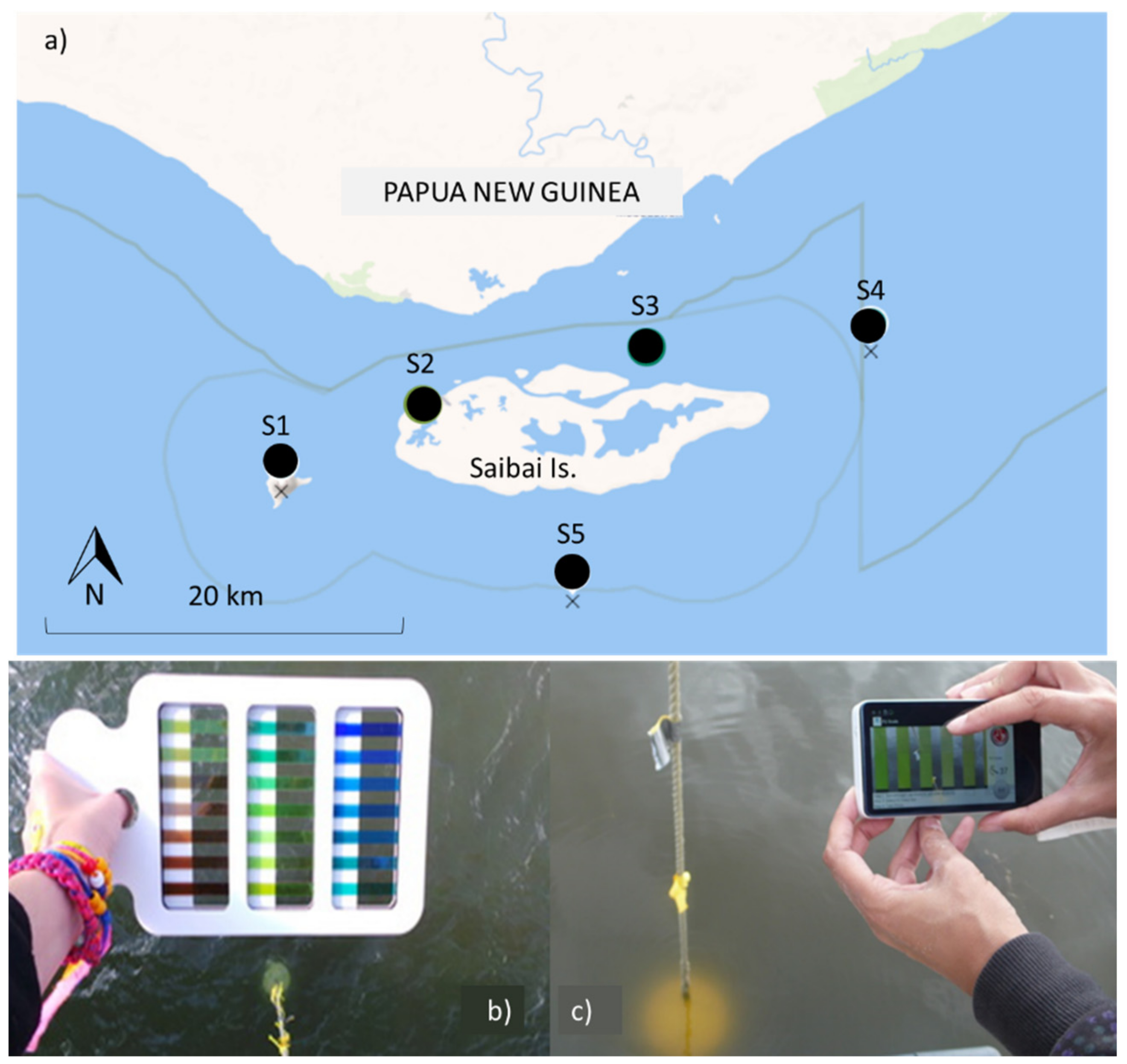
Appendix B.2. Optical Dataset

| Sample ID | Date | Lat | Long | Secchi (m) | SSC (mg/L) | Field FU |
|---|---|---|---|---|---|---|
| S1 | 12/11/2020 | −9.4 | 142.5 | 0.9 | 15 | 7 |
| S2 | 12/11/2020 | −9.4 | 142.6 | 0.7 | 25 | 15 |
| S3 | 12/11/2020 | −9.3 | 142.7 | 1.4 | 7.7 | 8 |
| S4 | 12/11/2020 | −9.3 | 142.9 | 3.4 | 2.3 | 6 |
| S5 | 12/11/2020 | −9.5 | 142.7 | 4.5 | 0.75 | 5 |
| S5 Duplicate | 12/11/2020 | −9.5 | 142.7 | 4.5 | 1.6 | 5 |
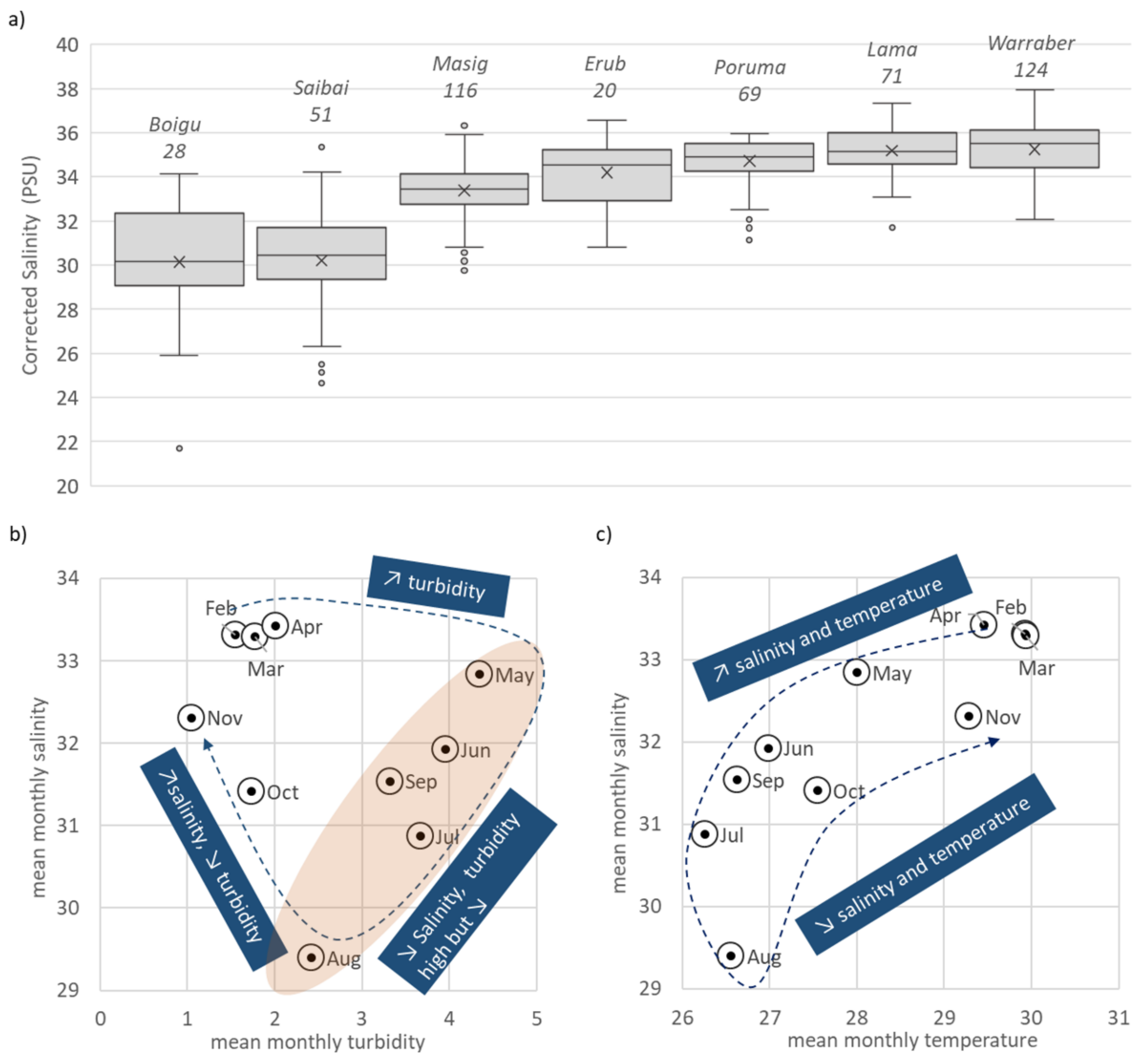
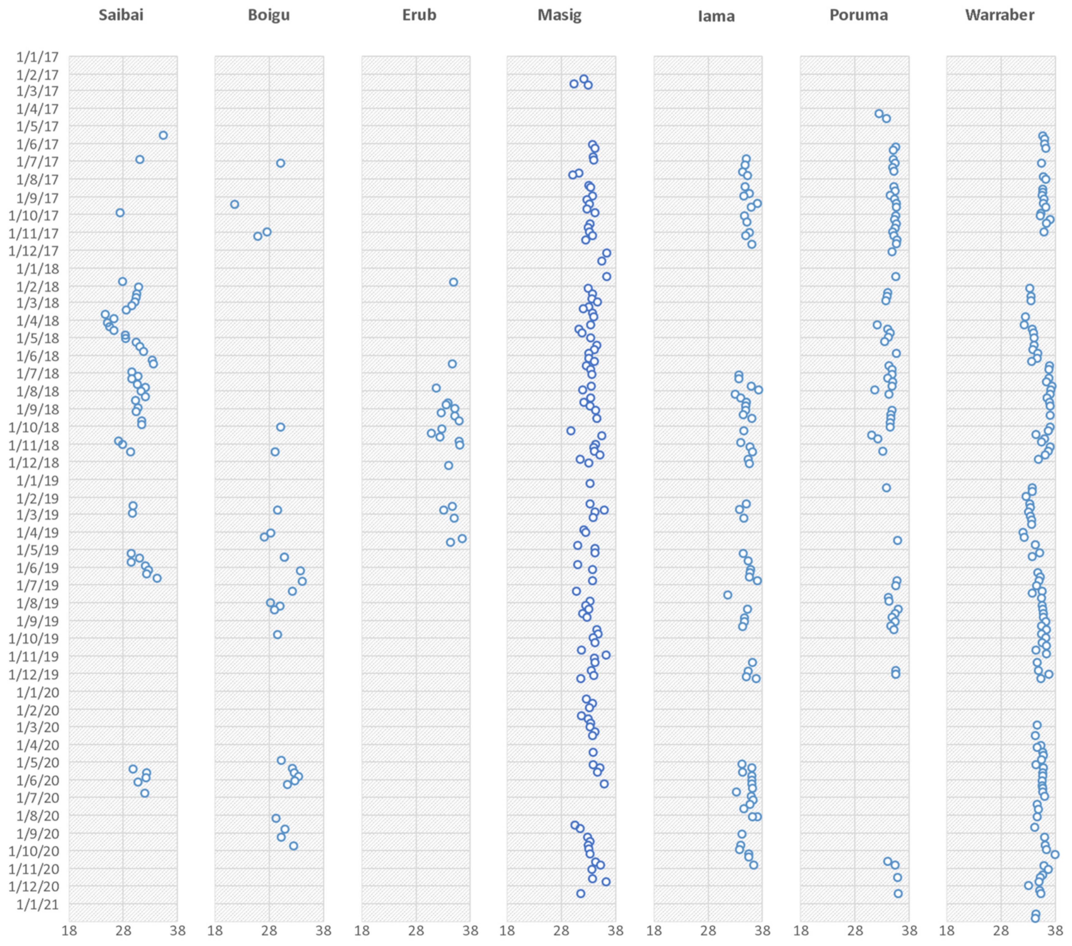
Appendix B.3. Salinity Monitoring

| Saibai | Boigu | Erub | Masig | Iama | Poruma | Warraber | |
|---|---|---|---|---|---|---|---|
| count | 51 | 28 | 20 | 116 | 71 | 69 | 124 |
| mean | 29.8 | 30.1 | 34.2 | 33.4 | 35.2 | 34.7 | 35.3 |
| median | 30.4 | 30.2 | 34.5 | 33.4 | 35.1 | 34.9 | 35.5 |
| sd | 2.2 | 2.6 | 1.5 | 1.3 | 1.0 | 1.0 | 1.2 |
| min | 24.6 | 21.7 | 30.8 | 29.8 | 31.7 | 31.1 | 32.1 |
| max | 35.3 | 34.1 | 36.6 | 36.4 | 37.3 | 36.0 | 37.9 |
| range | 10.7 | 12.4 | 5.7 | 6.7 | 5.7 | 4.8 | 5.9 |
| Q1 | 29.4 | 29.1 | 33.0 | 32.8 | 34.6 | 34.3 | 34.4 |
| Q3 | 31.6 | 32.3 | 35.2 | 34.1 | 36.0 | 35.5 | 36.1 |
Appendix B.4. Continuous Logger Data
| Salinity (PSU) | Temperature (°C) | Turbidity (NTU) | ||||
|---|---|---|---|---|---|---|
| Mean | SD | Mean | SD | Mean | SD | |
| February | 33.31 | 0.31 | 29.93 | 0.41 | 1.55 | 0.87 |
| March | 33.29 | 0.22 | 29.94 | 0.51 | 1.77 | 1.03 |
| April | 33.42 | 0.56 | 29.46 | 0.40 | 2.01 | 1.31 |
| May | 32.84 | 1.52 | 28.00 | 0.50 | 4.35 | 4.00 |
| June | 31.92 | 1.45 | 26.99 | 0.32 | 3.96 | 2.99 |
| July | 30.87 | 1.64 | 26.26 | 0.27 | 3.67 | 2.87 |
| August | 29.40 | 1.75 | 26.56 | 0.52 | 2.41 | 2.45 |
| September | 31.54 | 1.23 | 26.63 | 0.42 | 3.32 | 1.94 |
| October | 31.41 | 1.34 | 27.55 | 0.75 | 1.73 | 1.21 |
| November | 32.31 | 0.05 | 29.29 | 0.50 | 1.05 | 0.27 |
| February–November | 31.94 | 1.80 | 27.83 | 1.45 | 2.80 | 2.56 |
Appendix C. Median Composites

Appendix D. Decadal Monthly Difference Maps


References
- Halpern, B.S.; Frazier, M.; Potapenko, J.; Casey, K.S.; Koenig, K.; Longo, C.; Lowndes, J.S.; Rockwood, R.C.; Selig, E.R.; Selkoe, K.A.; et al. Spatial and temporal changes in cumulative human impacts on the world’s ocean. Nat. Commun. 2015, 6, 7615. [Google Scholar] [CrossRef] [PubMed] [Green Version]
- Thrush, S.F.; Hewitt, J.E.; Cummings, V.J.; Ellis, J.I.; Hatton, C.; Lohrer, A.; Norkko, A.J.F.I.E. Muddy waters: Elevating sediment input to coastal and estuarine habitats. Front. Ecol. Environ. 2004, 2, 299–306. [Google Scholar] [CrossRef]
- Romero, E.; Garnier, J.; Lassaletta, L.; Billen, G.; Le Gendre, R.; Riou, P.; Cugier, P. Large-scale patterns of river inputs in southwestern Europe: Seasonal and interannual variations and potential eutrophication effects at the coastal zone. Biogeochemistry 2013, 113, 481–505. [Google Scholar] [CrossRef] [Green Version]
- Halpern, B.S.; Walbridge, S.; Selkoe, K.A.; Kappel, C.V.; Micheli, F.; D’Agrosa, C.; Bruno, J.F.; Casey, K.S.; Ebert, C.; Fox, H.E.; et al. A global map of human impact on marine ecosystems. Science 2008, 319, 948–952. [Google Scholar] [CrossRef] [Green Version]
- Pockley, P. Global warming identified as main threat to coral reefs. Nature 2000, 407, 932. [Google Scholar] [CrossRef]
- Wolff, N.H.; Mumby, P.J.; Devlin, M.; Anthony, K.R. Vulnerability of the Great Barrier Reef to climate change and local pressures. Glob. Chang. Biol. 2018, 24, 1978–1991. [Google Scholar] [CrossRef] [Green Version]
- Brodie, J.; Lewis, S.; Collier, C.J.; Wooldridge, S.; Bainbridge, Z.; Waterhouse, J.; Rasheed, M.A.; Carol Honchin, C.; Holmes, G.; Fabricius, K. Setting ecologically relevant targets for river pollutant loads to meet marine water quality requirements for the Great Barrier Reef, Australia: A preliminary methodology and analysis. Ocean Coast. Manag. 2017, 143, 136–147. [Google Scholar] [CrossRef]
- Klein, C.J.; Ban, N.C.; Halpern, B.S.; Beger, M.; Game, E.T.; Grantham, H.S.; Green, A.; Kelin, T.J.; Kinninmonth, S.; Treml, E.; et al. Prioritizing land and sea conservation investments to protect coral reefs. PLoS ONE 2010, 5, 12431. [Google Scholar] [CrossRef] [Green Version]
- Brown, C.J.; Jupiter, S.D.; Albert, S.; Klein, C.J.; Mangubhai, S.; Maina, J.M.; Mumby, P.; Olley, J.; Stewart-Koster, B.; Tullock, V.; et al. Tracing the influence of land-use change on water quality and coral reefs using a Bayesian model. Sci. Rep. 2017, 7, 1–10. [Google Scholar] [CrossRef] [Green Version]
- Maina, J.; de Moel, H.; Vermaat, J.E.; Bruggemann, J.H.; Guillaume, M.M.; Grove, C.A.; Madin, J.S.; Mertz-Kraus, R.; Zinke, J. Linking coral river runoff proxies with climate variability, hydrology and land-use in Madagascar catchments. Mar. Pollut. Bull. 2012, 64, 2047–2059. [Google Scholar] [CrossRef]
- Petus, C.; Collier, C.; Devlin, M.; Rasheed, M.; McKenna, S. Using MODIS data for understanding changes in seagrass meadow health: A case study in the Great Barrier Reef (Australia). Mar. Environ. Res. 2014, 98, 68–85. [Google Scholar] [CrossRef]
- Petus, C.; Teixeira da Silva, E.; Devlin, M.; Wenger, A.; Álvarez-Romero, J.G. Using MODIS data for mapping of water types within river plumes in the Great Barrier Reef, Australia: Towards the production of river plume risk maps for reef and seagrass ecosystems. J. Environ. Manag. 2014, 137, 163–177. [Google Scholar] [CrossRef] [Green Version]
- Petus, C.; Devlin, M.; Thompson, A.; McKenzie, L.; Collier, C.; Teixeira da Silva, E.; Tracey, D. Estimating the Exposure of Coral Reefs and Seagrass Meadows to Land-Sourced Contaminants in River Flood Plumes of the Great Barrier Reef: Validating a Simple Satellite Risk Framework with Environmental Data. Remote Sens. 2016, 8, 210. [Google Scholar] [CrossRef] [Green Version]
- Petus, C.; Waterhouse, J.; Lewis, S.; Vacher, M.; Tracey, D.; Devlin, M. A flood of information: Using Sentinel-3 water colour products to assure continuity in the monitoring of water quality trends in the Great Barrier Reef (Australia). J. Environ. Manag. 2019, 2548, 109255. [Google Scholar] [CrossRef]
- Devlin, M.; Smith, A.; Graves, C.; Petus, C.; Tracey, D.; Maniel, M.; Hooper, E.; Kotra, K.; Samie, E.; Lyons, B. Baseline assessment of coastal water quality in Vanuatu, South Pacific: Insights gained from in-situ sampling. Mar. Pollut. Bull. 2020, 160, 111651. [Google Scholar] [CrossRef]
- Painting, S.J.; Collingridge, K.A.; Durand, D.; Grémare, A.; Créach, V.; Arvanitidis, C.; Bernard, G. Marine monitoring in Europe: Is it adequate to address environmental threats and pressures? Ocean Sci. 2020, 16, 235–252. [Google Scholar] [CrossRef] [Green Version]
- Devlin, M.; Petus, C.; Teixeira da Silva, E.; Tracey, D.; Wolff, N.; Waterhouse, J.; Brodie, J. Water Quality and River Plume monitoring in the Great Barrier Reef: An Overview of Methods Based on Ocean Colour Satellite Data. Remote Sens. 2015, 7, 12909–12941. [Google Scholar] [CrossRef] [Green Version]
- Le Traon, P.Y.; Reppucci, A.; Fanjul, E.A.; Aouf, L.; Behrens, A.; Belmonte, M.; Bentamy, A.; Bertino, L.; Brando, V.E.; Kreiner, M.B.; et al. From observation to information and users: The Copernicus Marine Service perspective. Front. Mar. Sci. 2019, 6, 234. [Google Scholar] [CrossRef] [Green Version]
- McCarthy, M.J.; Colna, K.E.; El-Mezayen, M.M.; Laureano-Rosario, A.E.; Méndez-Lázaro, P.; Otis, D.B.; Toro-Farmer, G.; Vega-Rodriguez, M.; Muller-Karger, F.E. Satellite remote sensing for coastal management: A review of successful applications. J. Environ. Manag. 2017, 60, 323–339. [Google Scholar] [CrossRef]
- Waterhouse, J.; Gruber, R.; Logan, M.; Petus, C.; Howley, C.; Lewis, S.; Tracey, D.; James, C.; Mellors, J.; Tonin, H.; et al. Marine Monitoring Program: Annual Report for Inshore Water Quality Monitoring 2019–20. In Report for the Great Barrier Reef Marine Park Authority; Great Barrier Reef Marine Park Authority: Townsville, Australia, 2021; 200p. [Google Scholar]
- Wolanski, E.; King, B.; Galloway, D. Dynamics of the turbidity maximum in the Fly River estuary, Papua New Guinea. Estuar. Coast. Shelf Sci. 1995, 40, 321–337. [Google Scholar] [CrossRef]
- Waterhouse, J.; Apte, S.; Petus, C.; Bainbridge, S.; Wolanski, E.; Tracey, D.; Angel, B.M.; Jarolimek, C.V.; Brodie, J. NESP Project 5.14. Identifying water quality and ecosystem health threats to the Torres Strait from Fly River runoff. In Report to the National Environmental Science Programme; Reef and Rainforest Research Centre Limited: Cairns, Australia, 2021; 162p. [Google Scholar]
- Wolanski, E.; Petus, C.; Lambrechts, J.; Brodie, J.; Waterhouse, J.; Tracey, D. The intrusion of polluted Fly River mud into Torres Strait. Mar. Pollut. Bull. 2021, 166, 112243. [Google Scholar] [CrossRef]
- Angel, B.M.; Apte, S.C.; Simpson, S.L.; Jarolimek, C.V.; Jung, R.F. Behaviour of copper in the Fly River Estuary, Papua New Guinea. In CSIRO Water for a Healthy Country Technical Report; Prepared for Ok Tedi Mining Ltd.: Tabubil, Papua New Guinea, 2010; 45p. [Google Scholar]
- Angel, B.M.; Apte, S.C.; Simpson, S.L.; Jarolimek, C.V.; King, J.J. The behaviour of trace metals in the Fly Estuary, Papua New Guinea. In CSIRO Water for a Healthy Country Technical Report; EP14897; Prepared for Ok Tedi Mining Ltd.: Tabubil, Papua New Guinea, 2014; 91p. [Google Scholar]
- Waterhouse, J.; Petus, C.; Brodie, J.; Bainbridge, S.; Wolanski, E.; Dafforn, K.A.; Birrer, S.C.; Lough, J.; Tracey, D.; Johnson, J.E.; et al. NESP Project 2.2.1. Identifying water quality and ecosystem health threats to the Torres Strait and Far Northern GBR from runoff of the Fly River. In Report to the National Environmental Science Programme; Reef and Rainforest Research Centre Limited: Cairns, Australia, 2018; 162p. [Google Scholar]
- Waterhouse, J.; Apte, S.C.; Brodie, J.; Hunter, C.; Petus, C.; Bainbridge, S.; Wolanski, E.; Dafforn, K.A.; Lough, J.; Tracey, D.; et al. Identifying water quality and ecosystem health threats to the Torres Strait from runoff arising from mine-derived pollution of the Fly River: Synthesis Report for NESP TWQ Hub Project 2.2.1 and NESP TWQ Hub Project 2.2.2. In Report to the National Environmental Science Program; Reef and Rainforest Research Centre Limited: Cairns, Australia, 2019; 19p. [Google Scholar]
- Walsh, J.P.; Ridd, P.V. Processes, sediments, and stratigraphy of the Fly River Delta. In The Fly River, Papua New Guinea: Environmental Studies in an Impacted Tropical River System, Developments in Earth & Environmental Sciences; Bolton, B.R., Ed.; Elsevier: Burlington, MA, USA, 2009; Volume 9, pp. 153–176. [Google Scholar]
- Wolanski, E.; Gibbs, R.J. Flocculation of suspended sediment in the Fly River estuary, Papua New Guinea. J. Coast. Res. 1995, 11, 754–762. [Google Scholar]
- Harris, P.T.; Baker, E.K.; Cole, A.R.; Short, S.A. A preliminary study of sedimentation in the tidally dominated Fly River Delta, Gulf of Papua. Cont. Shelf Res. 1993, 13, 441–472. [Google Scholar] [CrossRef]
- Wolanski, E.; Pickard, G.L.; Jupp, D.L.B. River plumes, coral reefs and mixing in the Gulf of Papua and the northern Great Barrier Reef. Estuar. Coast. Shelf Sci. 1984, 18, 291–314. [Google Scholar] [CrossRef]
- O’Brien, D.; Mellors, J.; Petus, C.; Martins, F.; Wolanski, E.; Brodie, J. Monitoring and assessment of water quality threats to Torres Strait marine waters and ecosystems. In Tropwater Report 15/43; James Cook University: Townsville, Australia, 2015; 30p. [Google Scholar]
- Petus, C. Application of MODIS remote sensing imagery for monitoring turbid river plumes from Papua New Guinea in the Torres Strait Region: A test study. In Technical Report to the National Environmental Research Program; Tropical System Hub: Cairns, Australia, 2013; 20p. [Google Scholar]
- Lawrey, E.P.; Stewart, M. Mapping the Torres Strait reef and island features—Extending the GBR features (GBRMPA) dataset. In Report to the National Environmental Science Programme; Reef and Rainforest Research Centre Limited: Cairns, Australia, 2016; 117p. [Google Scholar]
- Carter, A.B.; Taylor, H.A.; Rasheed, M.A. Torres Strait Mapping: Seagrass Consolidation, 2002–2014; JCU Publication, Report no. 14/55; Centre for Tropical Water & Aquatic Ecosystem Research: Cairns, Australia, 2014; 47p. [Google Scholar]
- Carter, A.B.; Rasheed, M.A. Torres Strait Seagrass Long-term Monitoring: Dugong Sanctuary, Dungeness Reef and Orman Reefs. In Centre for Tropical Water & Aquatic Ecosystems, Research Report No. 18/17; James Cook University: Cairns, Australia, 2018; 35p. [Google Scholar]
- Margvelashvili, N.; Saint-Cast, F.; Condie, S. Numerical modelling of the suspended sediment transport in Torres Strait. Cont. Shelf Res. 2008, 28, 2241–2256. [Google Scholar] [CrossRef]
- Hemer, M.; Harris, P.T.; Coleman, R.; Hunter, J. Sediment mobility due to currents and waves in the Torres Strait–Gulf of Papua region. Cont. Shelf Res. 2004, 24, 2297–2316. [Google Scholar] [CrossRef]
- Wolanski, E. A high resolution model of the water circulation in Torres Strait. In NERP Project 4.4 Hazard Assessment for Water Quality Threats to Torres Strait Marine Waters, Ecosystems and Public Health; Supplementary Report for NERP Project 4.4; James Cook University: Douglas, Australia, 2013; 45p. [Google Scholar]
- Ogston, A.S.; Sternberg, R.W.; Nittrouer, C.A.; Martin, D.P.; Goni, M.; Crockett, J.S. Sediment delivery from the Fly River tidally dominated delta to the nearshore marine environment and the impact of El Niño. J. Geophys. Res. Earth Surf. 2008, 113, F01S11. [Google Scholar] [CrossRef] [Green Version]
- Li, Y.; Martins, F.; Wolanski, E. Sensitivity analysis of the physical dynamics of the Fly River plume in Torres Strait. Estuar. Coast. Shelf Sci. 2017, 194, 84–91. [Google Scholar] [CrossRef]
- Apte, S.C.; Angel, B.M.; Hunter, C.; Jarolimek, C.V.; Chariton, A.A.; King, J.; Murphy, N. Impacts of mine-derived contaminants on Torres Strait environments and communities. In Report to the National Environmental Science Program; Reef and Rainforest Research Centre Limited: Cairns, Australia, 2018; 126p. [Google Scholar]
- Lough, J.M. Coral Core Records of the North-East Torres Strait. In Report to the National Environmental Science Programme; Reef and Rainforest Research Centre Limited: Cairns, Australia, 2016; 24p. [Google Scholar]
- Balasubramanian, S.V.; Pahlevan, N.; Smith, B.; Binding, C.; Schalles, J.; Loisel, H.; Gurlin, D.; Greb, S.; Alikas, K.; Randla, M.; et al. Robust algorithm for estimating total suspended solids (TSS) in inland and nearshore coastal waters. Remote Sens. Environ. 2020, 246, 111768. [Google Scholar] [CrossRef]
- Novoa, S.; Doxaran, D.; Ody, A.; Vanhellemont, Q.; Lafon, V.; Lubac, B.; Gernez, P. Atmospheric corrections and multi-conditional algorithm for multi-sensor remote sensing of suspended particulate matter in low-to-high turbidity levels coastal waters. Remote Sens. 2017, 9, 61. [Google Scholar] [CrossRef] [Green Version]
- IOCCG. Uncertainties in Ocean Colour Remote Sensing; Mélin, F., Ed.; IOCCG Report Series, No. 18; International Ocean Colour Coordinating Group: Dartmouth, NS, Canada, 2019; 170p. [Google Scholar]
- Toming, K.; Kutser, T.; Uiboupin, R.; Arikas, A.; Vahter, K.; Paavel, B. Mapping Water Quality Parameters with Sentinel-3 Ocean and Land Colour Instrument imagery in the Baltic Sea. Remote Sens. 2017, 9, 1070. [Google Scholar] [CrossRef] [Green Version]
- Alvarez-Romero, J.; Devlin, M.; da Silva, E.; Petus, C.; Ban, N.; Pressey, R.; Kool, J.; Roberts, J.; Cerdeira-Estrada, S.; Wenger, A.; et al. A novel approach to model exposure of coastal-marine ecosystems to riverine flood plumes based on remote sensing techniques. J. Environ. Manag. 2013, 119, 194–207. [Google Scholar] [CrossRef] [Green Version]
- Wang, S.; Li, J.; Zhang, W.; Cao, C.; Zhang, F.; Shen, Q.; Zhang, B. A dataset of remote-sensed Forel-Ule Index for global inland waters during 2000–2018. Sci. Data 2021, 8, 26. [Google Scholar] [CrossRef]
- Ye, M.; Sun, Y. Review of the Forel–Ule Index based on in situ and remote sensing methods and application in water quality assessment. Environ. Sci. Pollut. Res. 2022, 29, 3024–13041. [Google Scholar] [CrossRef]
- Pitarch, J.; van der Woerd, H.J.; Brewin, R.J.; Zielinski, O. Optical properties of Forel-Ule water types deduced from 15 years of global satellite ocean color observations. Remote Sens. Environ. 2019, 231, 111249. [Google Scholar] [CrossRef]
- Fronkova, L.; Greenwood, N.; Martinez, R.; Graham, J.A.; Harrod, R.; Graves, C.A.; Devlin, M.J.; Petus, C. Can Forel-Ule act as a proxy of water quality in temperate waters? Application of the GBR work in the Liverpool Bay, UK. Remote Sens. 2022; in press. [Google Scholar]
- Chen, X.; Liu, L.; Zhang, X.; Li, J.; Wang, S.; Liu, D.; Duan, H.; Song, K. An Assessment of Water Color for Inland Water in China Using a Landsat 8-Derived Forel–Ule Index and the Google Earth Engine Platform. IEEE J. Sel. Top. Appl. Earth Obs. Remote Sens. 2021, 14, 5773–5785. [Google Scholar] [CrossRef]
- Busch, J.A.; Bardaji, R.; Ceccaroni, L.; Friedrichs, A.; Piera, J.; Simon, C.; Thijsse, P.; Wernand, M.; Van der Woerd, H.; Zielinski, O. Citizen Bio-Optical Observations from Coast- and Ocean and Their Compatibility with Ocean Colour Satellite Measurements. Remote Sens. 2016, 8, 879. [Google Scholar] [CrossRef] [Green Version]
- Li, J.; Wang, S.; Wu, Y.; Zhang, B.; Chen, X.; Zhang, F.; Shen, Q.; Peng, D.; Tian, L. MODIS observations of water color of the largest 10 lakes in China between 2000 and 2012. Int. J. Digit. Earth 2016, 9, 788–805. [Google Scholar] [CrossRef]
- Wernand, M.R.; van der Woerd, H.J.; Gieskes, W.W.C. Trends in ocean colour and chlorophyll concentration from 1889 to 2000 worldwide. PLoS ONE 2013, 8, e63766. [Google Scholar] [CrossRef]
- Wang, S.; Li, J.; Zhang, B.; Lee, Z.; Spyrakos, E.; Feng, L.; Liu, C.; Zhao, H.; Wu, Y.; Zhu, L.; et al. Changes of water clarity in large lakes and reservoirs across china observed from long-term MODIS. Remote Sens. Environ. 2020, 247, 111949. [Google Scholar] [CrossRef]
- da Silva, E.F.F.; de Moraes Novo, E.M.L.; de Lucia Lobo, F.; Barbosa, C.C.F.; Cairo, C.T.; Noernberg, M.A.; da Silva Rotta, L.H. A machine learning approach for monitoring Brazilian optical water types using Sentinel-2 MSI. Remote Sens. Appl. Soc. Environ. 2021, 23, 100577. [Google Scholar]
- Torres Strait Regional Authority. Land and Sea Management Strategy for Torres Strait 2016–2036. In Report Prepared by the Land and Sea Management Unit; Torres Strait Regional Authority: Thursday Island, Australia, 2016; 104p. [Google Scholar]
- Sobtzick, S.; Hagihara, R.; Penrose, H.; Grech, A.; Cleguer, C.; Marsh, H. An assessment of the distribution and abundance of dugongs in the Northern Great Barrier Reef and Torres Strait. In A Report for the Department of the Environment, National Environmental Research Program (NERP); Reef and Rainforest Research Centre Limited: Cairns, Australia, 2014; 73p. [Google Scholar]
- Hamann, M.; Smith JPreston, S.; Fuentes, M.M.P.B. Nesting green turtles of Torres Strait. In Report to the National Environmental Research Program; Reef and Rainforest Research Centre Limited: Cairns, Australia, 2015; 13p. [Google Scholar]
- Johnson, J.E.; Welch, D.J.; Marshall, P.A.; Day, J.; Marshall, N.; Steinberg, C.R.; Benthuysen, J.A.; Sun, C.; Brodie, J.; Marsh, H.; et al. Characterising the values and connectivity of the northeast Australia seascape: Great Barrier Reef, Torres Strait, Coral Sea and Great Sandy Strait. In Report to the National Environmental Science Program; Reef and Rainforest Research Centre Limited: Cairns, Australia, 2018; 81p. [Google Scholar]
- Harris, P.T. Environmental Management of Torres Strait: A Marine Geologist’s Perspective. In Gondwana to Greenhouse: Environmental Geoscience—An Australian Perspective; Gostin, V.A., Ed.; Geological Society of Australia Special Publication: Adelaide, Australia, 2001; Volume 21, pp. 317–328. [Google Scholar]
- Devlin, M.; Schaffelke, B. Spatial extent of riverine flood plumes and exposure of marine ecosystems in the Tully coastal region, Great Barrier Reef. Mar. Freshw. Res. 2009, 60, 1109–1122. [Google Scholar] [CrossRef]
- Bainbridge, Z.; Lewis, S.; Stevens, T.; Petus, C.; Lazarus, E.; Gorman, J.; Smithers, S. Measuring sediment grain size across the catchment to reef continuum: Improved methods and environmental insights. Mar. Pollut. Bull. 2021, 168, 112339. [Google Scholar] [CrossRef]
- Collier, C.J.; Carter, A.B.; Rasheed, M.; McKenzie, L.; Udy, J.; Coles, R.; Lawrence, E. An evidence-based approach for setting desired state in a complex Great Barrier Reef seagrass ecosystem: A case study from Cleveland Bay. Environ. Dev. Sustain. 2020, 7, 100042. [Google Scholar] [CrossRef]
- Ceccarelli, D.M.; Evans, R.D.; Logan, M.; Mantel, P.; Puotinen, M.; Petus, C.; Russ, G.R.; Williamson, D.H. Long-term dynamics and drivers of coral and macroalgal cover on inshore reefs of the Great Barrier Reef Marine Park. Ecol. Appl. 2020, 30, e02008. [Google Scholar] [CrossRef] [Green Version]
- Wenger, A.S.; Williamson, D.H.; da Silva, E.T.; Ceccarelli, D.M.; Browne, N.K.; Petus, C.; Devlin, M.J. Effects of reduced water quality on coral reefs in and out of no-take marine reserves. Conserv. Biol. 2016, 30, 142–153. [Google Scholar] [CrossRef]
- Available online: https://eatlas.org.au/data/uuid/95338405-4b6f-4093-b278-04039e884136 (accessed on 8 April 2022).
- Wernand, M.R.; van der Woerd, H.J. Spectral analysis of the forel-ule ocean colour comparator scale. J. Eur. Opt. Soc. Rapid Publ. 2010, 5. Available online: http://www.jeos.org/index.php/jeos_rp/article/view/322 (accessed on 8 April 2022). [CrossRef] [Green Version]
- Wernand, M.R.; Hommersom, A.; van der Woerd, H.J. MERIS-based ocean colour classification with the discrete forel-ule scale. Ocean Sci. 2013, 9, 477–487. [Google Scholar] [CrossRef] [Green Version]
- Novoa, S.; Wernand, M.R.; Van der Woerd, H.J. The Forel-Ule scale revisited spectrally: Preparation protocol, transmission measurements and chromaticity. J. Eur. Opt. Soc. Rapid Publ. 2013, 8, 13057. [Google Scholar] [CrossRef] [Green Version]
- Available online: http://step.esa.int/main/toolboxes/sentinel-3-toolbox/s3tbx-features/ (accessed on 8 April 2022).
- Available online: https://www.sentinel-hub.com/explore/eobrowser/ (accessed on 8 April 2022).
- Available online: https://eatlas.org.au/data/uuid/c026de9e-bff4-4268-ad44-7c2e9bece110 (accessed on 8 April 2022).
- Available online: https://eatlas.org.au/data/uuid/03d84b70-d64c-4d89-846b-f1aa14f30ff7 (accessed on 8 April 2022).
- Available online: https://www.eyeonwater.org/observations (accessed on 8 April 2022).
- Novoa, S.; Wernand, M.R.; van der Woerd, H.J. Wacodi: A generic algorithm to derive the intrinsic color of natural waters from digital images. Limnol. Oceanogr. Methods 2015, 13, 697–711. [Google Scholar] [CrossRef] [Green Version]
- Malthus, T.J.; Ohmsen, R.; Van der Woerd, H.J. An Evaluation of citizen science smartphone apps for inland water quality assessment. Remote Sens. 2020, 12, 1578. [Google Scholar] [CrossRef]
- Available online: https://eatlas.org.au/data/uuid/44eb7285-296f-4fe9-b662-46899364029e (accessed on 8 April 2022).
- Wolanski, E.; Lambrechts, J.; Thomas, C.; Deleersnijder, E. The net water circulation through Torres Strait. Cont. Shelf Res. 2013, 64, 66–74. [Google Scholar] [CrossRef]
- Harris, P.T. Sediments, bedforms and bedload transport pathways on the continental shelf adjacent to Torres Strait, Australia—Papua New Guinea. Cont. Shelf Res. 1988, 8, 979–1003. [Google Scholar] [CrossRef]
- Heap, A.D.; Sbaffi, L. Composition and distribution of seabed and suspended sediments in north and central Torres Strait, Australia. Cont. Shelf Res. 2008, 16, 2174–2187. [Google Scholar] [CrossRef]
- Gladstone, W. Trace Metals in Sediments, Indicator Organisms and Traditional Seafoods of the Torres Strait; Great Barrier Reef Marine Park Authority: Townsville, Australia, 1996; 177p. [Google Scholar]
- Limpus, C.J.; Miller, J.D.; Parmenter, C.J.; Limpus, D.J. The Green Turtle, Chelonia mydas, Population of Raine Island and the Northern Great Barrier Reef: 1843–2001. Mem. Qld. Mus. 2003, 49, 349–440. [Google Scholar]
- King, B.R. The Status of Queensland Seabirds. Corella 1993, 17, 65–92. [Google Scholar]
- Begg, G.A.; Chen, C.C.M.; O’Neill, M.F.; Rose, D.B. Stock assessment of the Torres Strait Spanish mackerel fishery. CRC Reef Res. Cent. Tech. Rep. 2006, 66, 81. [Google Scholar]
- Commonwealth of Australia. Assessment of the Torres Strait Finfish Fishery; Department of Agriculture, Water and the Environment: Canberra, Australia, 2020; 54p.
- Marsh, H. Torres Strait Dugong 1998. In Fisheries Assessment Report, Edited by the Torres Strait Fisheries Assessment Group; Australian Fisheries Management Authority: Canberra, Australia, 1999; 23p. [Google Scholar]
- Brown, C.J.; Jupiter, S.D.; Albert, S.; Anthony, K.R.; Hamilton, R.J.; Fredston-Hermann, A.; Halpern, B.S.; Lin, H.-Y.; Maina, J.; Mangubhai, S.; et al. A guide to modelling priorities for managing land-based impacts on coastal ecosystems. J. Appl. Ecol. 2019, 56, 1106–1116. [Google Scholar] [CrossRef] [Green Version]
- Bohnet, I.C.; Kinjun, C. Community uses and values of water informing water quality improvement planning: A study from the Great Barrier Reef region, Australia. Mar. Freshw. Res. 2009, 60, 1176–1182. [Google Scholar] [CrossRef] [Green Version]
- Kaiser, B.A.; Hoeberechts, M.; Maxwell, K.; Eerkes-Medrano, L.; Hilmi, N.; Safa, A.; Horbel, C.; Juniper, S.K.; Roughan, M.; Theux Lowen, N.; et al. The importance of connected ocean monitoring knowledge systems and communities. Front. Mar. Sci. 2019, 6, 309. [Google Scholar] [CrossRef] [Green Version]


| Characteristics | Monsoon Season | Trade Wind Season |
|---|---|---|
| Time period | January to April | May to December: |
| Winds | NW monsoon—Typical wind speeds in the area are of order 9 knots | SE trade winds—typical wind speeds of over 20 knots. A period of relative calm (transition period) occurs between November and December with winds slowly veering and backing to northerly. |
| Waves | Offshore winds result in little or no long-period swell propagating towards the south coast of PNG. | TS is generally protected from surface waves by the northern-most extension of the GBR |
| Rainfall | Higher rainfall (median December–May = 1968 mm). Storms and infrequent tropical cyclones influence the inter-annual variability of the sediment fluxes | Lower rainfall (median June–November = 1345 mm) |
| Wind-driven currents | Eastward | Westward. Controls the westward transport of suspended sediments along the southern coast of PNG between Daru and Saibai Island. |
| Mean sea level (MSL) difference across the TS | Negative (MSL Gulf of Carpentaria > MSL Gul of Papua) | Positive (MSL Gulf of Carpentaria < MSL Gulf of Papua) |
| WS Colour Scale (GBR) | FU Colour Scale (Global) | Description | SCC (mg L−1) and SDD (m) Measured in the GBR | |
|---|---|---|---|---|
| Water Colour | OWT Name (WS Colour Classes) | OWT Name (FU Colour Classes) | ||
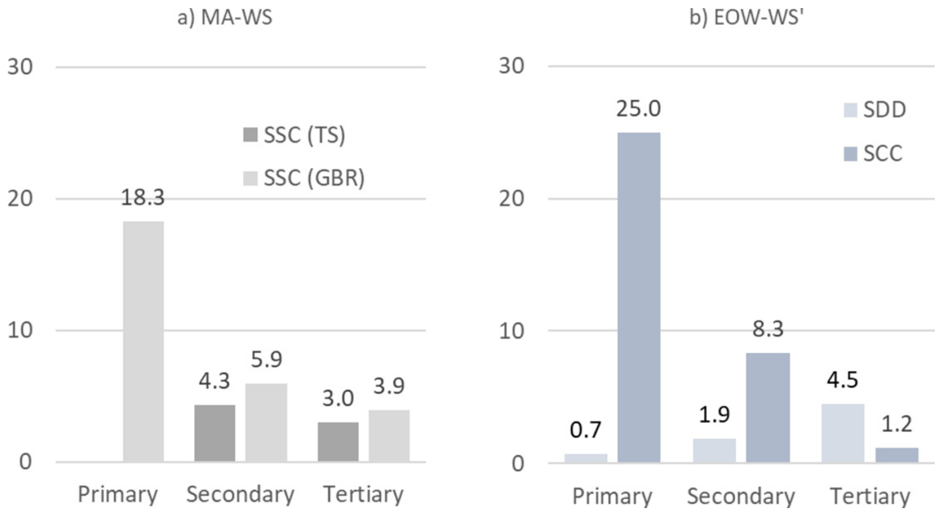
| Brownish to brownish-green | Primary (WS1-4) | Primary’ (FU ≥ 10) | Turbid waters with high SSC, but also enriched in chl-a, and CDOM resulting in reduced light levels. In the GBR, this OWT is typical of inshore regions that receive land-based discharge and have high concentrations of resuspended sediments during the wet season. | SCC: 18.3 ± 45.7 mg L−1 and SDD: 1.8 ± 1.7 m |
| Greenish to greenish-blue | Secondary (WS5) | Secondary’ (FU6-9) | Less turbid water typical of coastal waters rich in algae (Chl-a) and containing CDOM and fine sediment. In the GBR, this OWT is found in open coastal waters as well as in the mid-water regions of river plumes. | SCC: 5.9 ± 8.0 mg L−1 and SDD: 4.0 ± 2.3 m |
| Greenish-blue | Tertiary (WS6) | Tertiary’ (FU4-5) | Low-turbidity waters with slightly above ambient optically active constituent concentrations. In the GBR, this OWT is typical of GBR areas towards the open sea and include offshore regions of river plumes, fine sediment resuspension around reefs and islands and marine processes such as upwellings. | SCC: 3.9 ± 5.1 mg L−1 and SDD: 7.0 ± 3.8 m |
| Blueish | Marine (WS7) | Marine’ (FU1-3) | Ambient waters with high light penetration and negligible levels of SSC, CDOM and Chl-a. | SCC: 2.2 ± 3.9 mg L−1 and SDD: 11.1 ± 5.1 m |
| Product | Objective | Time Scales | Production |
|---|---|---|---|
| (a) Composite Colour class map | Illustrate large scale spatial patterns in turbidity levels at different time scales | Decadal (2009–2018) | Decadal median maps are produced by calculating the median long-term colour class category value for each pixel of our study area using (i) all daily MA-WS data using data from 2009 to 2018, or using data collected in the (ii) monsoon and trade wind seasons or (iii) in each month of the 2009–2018 period |
| (b) Frequency maps | Assess the area of coral reefs and seagrasses that were regularly exposed to turbid waters. Evaluate the frequency of exposure of TS coral reefs and seagrass key habitats to Primary, Secondary and Tertiary water types | Annual and decadal average | The annual water type frequency was defined as the total number of days per year exposed to a given water type divided by the number of data days (non-cloud) recorded per year, resulting in a normalised frequency on a scale from 0 to 1. Decadal average were calculated as the average of all annual frequency maps. |
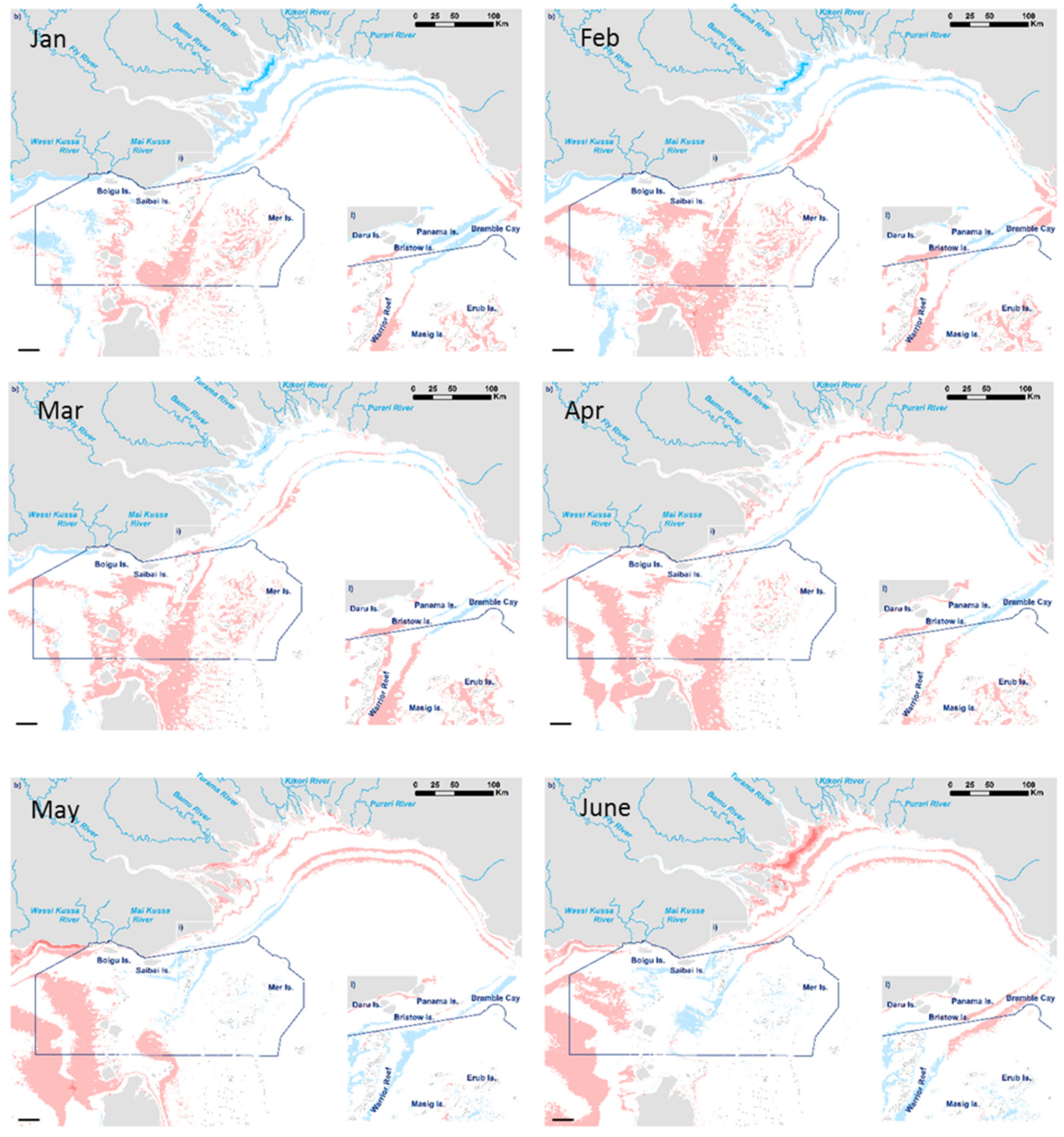
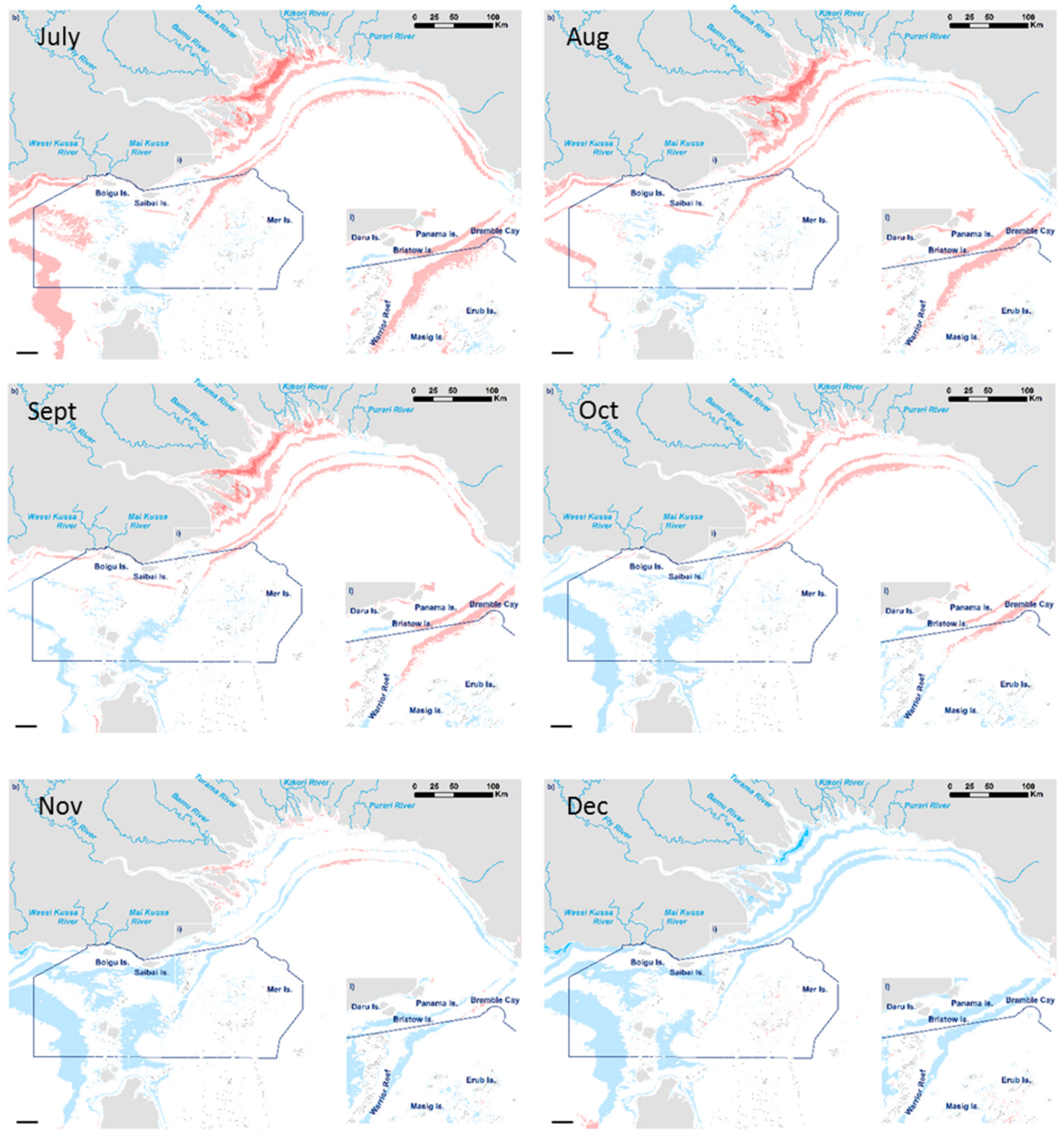
| (c) Difference maps | Illustrate areas with an increase (positive anomaly) or decrease (negative anomaly) in relative turbidity during the trade wind season against the monsoonal trends; or in each month against long-term trends | Decadal seasonal or Decadal monthly | The seasonal difference map is calculated by subtracting the median decadal monsoonal and the median decadal trade wind maps. The monthly difference maps are calculated by subtracting the median decadal monthly maps and the decadal median map. |
Publisher’s Note: MDPI stays neutral with regard to jurisdictional claims in published maps and institutional affiliations. |
© 2022 by the authors. Licensee MDPI, Basel, Switzerland. This article is an open access article distributed under the terms and conditions of the Creative Commons Attribution (CC BY) license (https://creativecommons.org/licenses/by/4.0/).
Share and Cite
Petus, C.; Waterhouse, J.; Tracey, D.; Wolanski, E.; Brodie, J. Using Optical Water-Type Classification in Data-Poor Water Quality Assessment: A Case Study in the Torres Strait. Remote Sens. 2022, 14, 2212. https://0-doi-org.brum.beds.ac.uk/10.3390/rs14092212
Petus C, Waterhouse J, Tracey D, Wolanski E, Brodie J. Using Optical Water-Type Classification in Data-Poor Water Quality Assessment: A Case Study in the Torres Strait. Remote Sensing. 2022; 14(9):2212. https://0-doi-org.brum.beds.ac.uk/10.3390/rs14092212
Chicago/Turabian StylePetus, Caroline, Jane Waterhouse, Dieter Tracey, Eric Wolanski, and Jon Brodie. 2022. "Using Optical Water-Type Classification in Data-Poor Water Quality Assessment: A Case Study in the Torres Strait" Remote Sensing 14, no. 9: 2212. https://0-doi-org.brum.beds.ac.uk/10.3390/rs14092212